
The concept behind clustering in a data stream remains the same as in batch or offline modes; that is, finding interesting clusters or patterns which group together in the data while keeping the limits on finite memory and time required to process as constraints. Doing single-pass modifications to existing algorithms or keeping a small memory buffer to do mini-batch versions of existing algorithms, constitute the basic changes done in all the algorithms to make them suitable for stream or real-time unsupervised learning.
The clustering modeling techniques for online learning are divided into partition-based, hierarchical-based, density-based, and grid-based, similar to the case of batch-based clustering.
The concept of partition-based algorithms is similar to batch-based clustering where k clusters are formed to optimize certain objective functions such as minimizing the inter-cluster distance, maximizing the intra-cluster distance, and so on.
k-Means is the most popular clustering algorithm, which partitions the data into user-specified k clusters, mostly to minimize the squared error or distance between centroids and cluster assigned points. We will illustrate a very basic online adaptation of k-Means, of which several variants exist.
Mainly, numeric features are considered as inputs; a few tools take categorical features and convert them into some form of numeric representation. The algorithm itself takes the parameters' number of clusters k and number of max iterations n as inputs.
- The input data stream is considered to be infinite but of constant block size.
- A memory buffer of the block size is kept reserved to store the data or a compressed representation of the data.
- Initially, the first stream of data of block size is used to find the k centroids of the clusters, the centroid information is stored and the buffer is cleared.
- For the next data after it reaches the block size:
- For either max number of iterations or until there is no change in the centroids:
- Execute k-Means with buffer data and the present centroids.
- Minimize the squared sum error between centroids and data assigned to the cluster.
- After the iterations, the buffer is cleared and new centroids are obtained.
- Repeat step 4 until the data is no longer available.
The advantages and limitations are as follows:
- Similar to batch-based, the shape of the detected cluster depends on the distance measure and is not appropriate in problem domains with irregular shapes.
- The choice of parameter k, as in batch-based, can limit the performance in datasets with many distinct patterns or clusters.
- Outliers and missing data can pose lots of irregularities in clustering behavior of online k-Means.
- If the selected buffer size or the block size of the stream on which iterative k-Means runs is small, it will not find the right clusters. If the chosen block size is large, it can result in slowdown or missed changes in the data. Extensions such as Very Fast k-Means Algorithm (VFKM), which uses the Hoeffding bound to determine the buffer size, overcome this limitation to a large extent.
Hierarchical methods are normally based on Clustering Features (CF) and Clustering Trees (CT). We will describe the basics and elements of hierarchical clustering and the BIRCH algorithm, the extension of which the CluStream algorithm is based on.
The Clustering Feature is a way to compute and preserve a summarization statistic about the cluster in a compressed way rather than holding on to the whole data belonging to the cluster. In a d dimensional dataset, with N points in the cluster, two aggregates in the form of total sum LS for each dimensions and total squared sum of data SS again for each dimension, are computed and the vector representing this triplet form the Clustering Feature:
CFj = < N, LSj, SSj >
These statistics are useful in summarizing the entire cluster information. The centroid of the cluster can be easily computed using:
centroidj = LSj/N
The radius of the cluster can be estimated using:

The diameter of the cluster can be estimated using:

CF vectors have great incremental and additive properties which becomes useful in stream or incremental updates.
For an incremental update, when we must update the CF vector, the following holds true:


When two CFs have to be merged, the following holds true:
The Clustering Feature Tree (CF Tree) represents an hierarchical tree structure. The construction of the CF tree requires two user defined parameters:
- Branching factor b which is the maximum number of sub-clusters or non-leaf nodes any node can have
- Maximum diameter (or radius) T, the number of examples that can be absorbed by the leaf node for a CF parent node
CF Tree operations such as insertion are done by recursively traversing the CF Tree and using the CF vector for finding the closest node based on distance metrics. If a leaf node has already absorbed the maximum elements given by parameter T, the node is split. At the end of the operation, the CF vector is appropriately updated for its statistic:

Figure 3 An example Clustering Feature Tree illustrating hierarchical structure.
We will discuss BIRCH (Balanced Iterative Reducing and Clustering Hierarchies) following this concept.
BIRCH only accepts numeric features. CF and CF tree parameters, such as branching factor b and maximum diameter (or radius) T for leaf are user-defined inputs.
BIRCH, designed for very large databases, was meant to be a two-pass algorithm; that is, scan the entire data once and re-scan it again, thus being an O(N) algorithm. It can be modified easily enough for online as a single pass algorithm preserving the same properties:
- In the first phase or scan, it goes over the data and creates an in-memory CF Tree structure by sequentially visiting the points and carrying out CF Tree operations as discussed previously.
- In the second phase, an optional phase, we remove outliers and merge sub-clusters.
- Phase three is to overcome the issue of order of data in phase one. We use agglomerative hierarchical clustering to refactor the CF Tree.
- Phase four is the last phase which is an optional phase to compute statistics such as centroids, assign data to closest centroids, and so on, for more effectiveness.
The advantages and limitations are as follows:
- It is one of the most popular algorithms that scales linearly on a large database or stream of data.
- It has compact memory representation in the form of the CF and CF Tree for statistics and operations on incoming data.
- It handles outliers better than most algorithms.
- One of the major limitations is that it has been shown not to perform well when the shape of the clusters is not spherical.
- The concepts of CF vector and clustering in BIRCH were extended for efficient stream mining requirements by Aggarwal et al and named micro-cluster and CluStream.
CluStream only accepts numeric features. Among the user-defined parameters are the number of micro-clusters in memory (q) and the threshold (δ) in time after which they can be deleted. Additionally, included in the input are time-sensitive parameters for storing the micro-clusters information, given by α and l.
- The micro-cluster extends the CF vector and keeps two additional measures. They are the sum of the timestamps and sum of the squares of timestamps:
microClusterj = < N, LSj, SSj, ST, SST>
- The algorithm stores q micro-clusters in memory and each micro-cluster has a maximum boundary that can be computed based on means and standard deviations between centroid and cluster instance distances. The measures are multiplied by a factor which decreases exponentially with time.
- For each new instance, we select the closest micro-cluster based on Euclidean distance and decide whether it should be absorbed:
- If the distance between the new instance and the centroid of the closest micro-cluster falls within the maximum boundary, it is absorbed and the micro-cluster statistics are updated.
- If none of the micro-clusters can absorb, a new micro-cluster is created with the instance and based on the timestamp and threshold (δ), the oldest micro-cluster is deleted.
- Assuming normal distribution of timestamps, if the relevance time—the time of arrival of instance found by CluStream—is below the user-specified threshold, it is considered an outlier and removed. Otherwise, the two closest micro-clusters are merged.
- The micro-cluster information is stored in secondary storage from time to time by using a pyramidal time window concept. Each micro-cluster has time intervals decrease exponentially using αl to create snapshots. These help in efficient search in both time and space.
The advantages and limitations are as follows:
Similar to batch clustering, density-based techniques overcome the "shape" issue faced by distance-based algorithms. Here we will present a well-known density-based algorithm, DenStream, which is based on the concepts of CF and CF Trees discussed previously.
The extent of the neighborhood of a core micro-cluster is the user-defined radius ϵ. A second input value is the minimum total weight µ of the micro-cluster which is the sum over the weighted function of the arrival time of each instance in the object, where the weight decays with a time constant proportional to another user-defined parameter, λ. Finally, an input factor β ∈ (0,1) is used to distinguish potential core micro-clusters from outlier micro-clusters.
- Based on the micro-cluster concepts of CluStream, DenStream holds two data structures: p-micro-cluster for potential clusters and o-micro-clusters for outlier detection.
- Each p-micro-cluster structure has:
-
A weight associated with it which decreases exponentially with the timestamps it has been updated with. If there are j objects in the micro-cluster:
 where f(t) = 2-λt
 - Weighted linear sum (WLS) and weighted linear sum of squares (WSS) are stored in micro-clusters similar to linear sum and sum of squares:


- The mean, radius, and diameter of the clusters are then computed using the weighted measures defined previously, exactly like in CF. For example, the radius can be given as:

-
A weight associated with it which decreases exponentially with the timestamps it has been updated with. If there are j objects in the micro-cluster:
- Each o-micro-cluster has the same structure as p-micro-cluster and timestamps associated with it.
- When a new instance arrives:
- A closest p-micro-cluster is found and the instance is inserted if the new radius is within the user-defined boundary ϵ. If inserted, the p-micro-cluster statistics are updated accordingly.
- Otherwise, an o-micro-cluster is found and the instance is inserted if the new radius is again within the boundary. The boundary is defined by β × μ, the product of the user-defined parameters, and if the radius grows beyond this value, the o-micro-cluster is moved to the p-micro-cluster.
- If the instance cannot be absorbed by an o-micro-cluster, then a new micro-cluster is added to the o-micro-clusters.
- At the time interval t based on weights, the o-micro-cluster can become the p-micro-cluster or vice versa. The time interval is defined in terms of λ, β, and µ as:

The advantages and limitations are as follows:
- Based on the parameters, DenStream can find effective clusters and outliers for real-time data.
- It has the advantage of finding clusters and outliers of any shape or size.
- The house keeping job of updating the o-micro-cluster and p-micro-cluster can be computationally expensive if not selected properly.
This technique is based on discretizing the multi-dimensional continuous space into a multi-dimensional discretized version with grids. The mapping of the incoming instance to grid online and maintaining the grid offline results in an efficient and effective way of finding clusters in real-time.
Here we present D-Stream, which is a grid-based online stream clustering algorithm.
As in density-based algorithms, the idea of decaying weight of instances is used in D-Stream. Additionally, as described next, cells in the grid formed from the input space may be deemed sparse, dense, or sporadic, distinctions that are central to the computational and space efficiency of the algorithm. The inputs to the grid-based algorithm, then, are:
- Each instance arriving at time t has a density coefficient that decreases exponentially over time:

- Density of the grid cell g at any given time t is given by D(g, t) and is the sum of the adjusted density of all instances given by E(g, t) that are mapped to grid cell g:

- Each cell in the grid captures the statistics as a characterization vector given by:
- CV(g) = <tg, t>m, D, label, status> where:
- tg = last time grid cell was updated
- tm = last time grid cell was removed due to sparseness
- D = density of the grid cell when last updated
- label = class label of the grid cell
- status = {NORMAL or SPORADIC}
- When the new instance arrives, it gets mapped to a cell g and the characteristic vector is updated. If g is not available, it is created and the list of grids is updated.
- Grid cells with empty instances are removed. Also, cells that have not been updated over a long time can become sparse, and conversely, when many instances are mapped, they become dense.
- At a regular time interval known as a gap, the grid cells are inspected for status and the cells with fewer instances than a number—determined by a density threshold function—are treated as outliers and removed.
Many of the static clustering evaluation measures discussed in Chapter 3, Unsupervised Machine Learning Techniques, have an assumption of static and non-evolving patterns. Some of these internal and external measures are used even in streaming based cluster detection. Our goal in this section is to first highlight problems inherent to cluster evaluation in stream learning, then describe different internal and external measures that address these, and finally, present some existing measures—both internal and external—that are still valid.
It is important to understand some of the important issues that are specific to streaming and clustering, as the measures need to address them:
- Aging: The property of points being not relevant to the clustering measure after a given time.
- Missed points: The property of a point not only being missed as belonging to the cluster but the amount by which it was missed being in the cluster.
- Misplaced points: Changes in clusters caused by evolving new clusters. Merging existing or deleting clusters results in ever-misplaced points with time. The impact of these changes with respect to time must be taken into account.
- Cluster noise: Choosing data that should not belong to the cluster or forming clusters around noise and its impact over time must be taken into account.
Evaluation measures for clustering in the context of streaming data must provide a useful index of the quality of clustering, taking into consideration the effect of evolving and noisy data streams, overlapping and merging clusters, and so on. Here we present some external measures used in stream clustering. Many internal measures encountered in Chapter 3, Unsupervised Machine Learning Techniques, such as the Silhouette coefficient, Dunn's Index, and R-Squared, are also used and are not repeated here.
The idea behind CMM is to quantify the connectivity of the points to clusters given the ground truth. It works in three phases:
Mapping phase: In this phase, clusters assigned by the stream learning algorithm are mapped to the ground truth clusters. Based on these, various statistics of distance and point connectivity are measured using the concepts of k-Nearest Neighbors.
The average distance of point p to its closest k neighbors in a cluster Ci is given by:

The average distance for a cluster Ci is given by:

The point connectivity of a point p in a cluster Ci is given by:
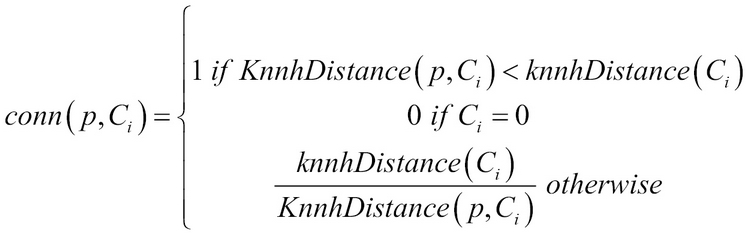
Class frequencies are counted for each cluster and the mapping of the cluster to the ground truth is performed by calculating the histograms and similarity in the clustering.
Specifically, a cluster Ci is mapped to the ground truth class, and Clj is mapped to a ground truth cluster ![]() , which covers the majority of class frequencies of Ci. The surplus is defined as the number of instances from class Cli not covered by the ground truth cluster
, which covers the majority of class frequencies of Ci. The surplus is defined as the number of instances from class Cli not covered by the ground truth cluster ![]() and total surplus for instances in classes Cl1, Cl2, Cl3 … Cl1 in cluster Ci compared to
and total surplus for instances in classes Cl1, Cl2, Cl3 … Cl1 in cluster Ci compared to ![]() is given by:
is given by:

Cluster Ci is mapped using:

Penalty phase: The penalty for every instance that is mapped incorrectly is calculated in this step using computations of fault objects; that is, objects which are not noise and yet incorrectly placed, using:

The overall penalty of point o with respect to all clusters found is given by:

CMM calculation: Using all the penalties weighted over the lifespan is given by:
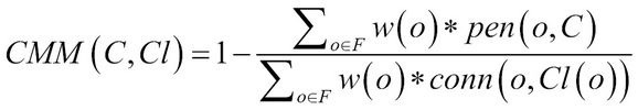
Here, C is found clusters, Cl is ground truth clusters, F is the fault objects and w(o) is the weight of instance.
Validity or V-Measure is an external measure which is computed based on two properties that are of interest in stream clustering, namely, Homogeneity and Completeness. If there are n classes as set C = {c1, c2 …, cn} and k clusters K = {k1, k2..km}, contingency tables are created such that A = {aij} corresponds to the count of instances in class ci and cluster kj.
Homogeneity: Homogeneity is defined as a property of a cluster that reflects the extent to which all the data in the cluster belongs to the same class.
Conditional entropy and class entropy:


Homogeneity is defined as:

A higher value of homogeneity is more desirable.
Completeness: Completeness is defined as the mirror property of Homogeneity, that is, having all instances of a single class belong to the same cluster.
Similar to Homogeneity, conditional entropies and cluster entropy are defined as:


Completeness is defined as:

V-Measure is defined as the harmonic mean of homogeneity and completeness using a weight factor β:

A higher value of completeness or V-measure is better.
Some external measures which are quite popular in comparing the clustering algorithms or measuring the effectiveness of clustering when the classes are known are given next:
Purity and Entropy: They are similar to homogeneity and completeness defined previously.

Entropy is defined as:
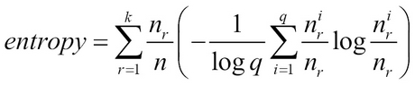
Here, q = number of classes, k = number of clusters, nr = size of cluster r and ![]() .
.
Precision, Recall, and F-Measure: Information retrieval measures modified for clustering algorithms are as follows:
Given, ![]() and
and ![]() .
.

Recall is defined as:

F-measures is defined as:
