
Grubbs, in 1969, offers the definition, "An outlying observation, or outlier, is one that appears to deviate markedly from other members of the sample in which it occurs".
Hawkins, in 1980, defined outliers or anomaly as "an observation which deviates so much from other observations as to arouse suspicions that it was generated by a different mechanism".
Barnett and Lewis, 1994, defined it as "an observation (or subset of observations) which appears to be inconsistent with the remainder of that set of data".
Outlier detection techniques are classified based on different approaches to what it means to be an outlier. Each approach defines outliers in terms of some property that sets apart some objects from others in the dataset:
- Statistical-based: This is improbable according to a chosen distribution
- Distance-based: This is isolated from neighbors according to chosen distance measure and fraction of neighbors within threshold distance
- Density-based: This is more isolated from its neighbors than they are in turn from their neighbors
- Clustering-based: This is in isolated clusters relative to other clusters or is not a member of any cluster
- High-dimension-based: This is an outlier by usual techniques after data is projected to lower dimensions, or by choosing an appropriate metric for high dimensions
Statistical-based techniques that use parametric methods for outlier detection assume some knowledge of the distribution of the data (References [19]). From the observations, the model parameters are estimated. Data points that have probabilities lower than a threshold value in the model are considered outliers. When the distribution is not known or none is suitable to assume, non-parametric methods are used.
Statistical methods for outlier detection work with real-valued datasets. The choice of distance metric may be a user-selected input in the case of parametric methods assuming multivariate distributions. In the case of non-parametric methods using frequency-based histograms, a user-defined threshold frequency is used. Selection of kernel method and bandwidth are also user-determined in Kernel Density Estimation techniques. The output from statistical-based methods is a score indicating outlierness.
Most of the statistical-based outlier detections either assume a distribution or fit a distribution to the data to detect probabilistically the least likely data generated from the distribution. These methods have two distinct steps:
- Training step: Here, an estimate of the model to fit the data is performed
- Testing step: On each instance a goodness of fit is performed based on the model and the particular instance, yielding a score and the outlierness
Parametric-based methods assume a distribution model such as multivariate Gaussians and the training normally involves estimating the means and variance using techniques such as Maximum Likelihood Estimates (MLE). The testing typically includes techniques such as mean-variance or box-plot tests, accompanied by assumptions such as "if outside three standard deviations, then outlier".
A normal multivariate distribution can be estimated as:

with the mean µ and covariance Ʃ.
The Mahalanobis distance can be the estimate of the data point from the distribution given by the equation ![]() . Some variants such as Minimum Covariant Determinant (MCD) are also used when Mahalanobis distance is affected by outliers.
. Some variants such as Minimum Covariant Determinant (MCD) are also used when Mahalanobis distance is affected by outliers.
A non-parametric method involves techniques such as constructing histograms for every feature using frequency or width-based methods. When the ratio of the data in a bin to that of the average over the histogram is below a user defined threshold, such a bin is termed sparse. A lower probability of feature results in a higher outlier score. The total outlier score can be computed as:

Here, wf is the weight given to feature f, pf is the probability of the value of the feature in the test data point, and F is the sum of weights of the feature set. Kernel Density Estimations are also used in non-parametric methods using user-defined kernels and bandwidth.
- When the model fits or distribution of the data is known, these methods are very efficient as you don't have to store entire data, just the key statistics for doing tests.
- Assumptions of distribution, however, can pose a big issue in parametric methods. Most non-parametric methods using kernel density estimates don't scale well with large datasets.
Distance-based algorithms work under the general assumption that normal data has other data points closer to it while anomalous data is well isolated from its neighbors (References [20]).
Distance-based techniques require natively numeric or categorical features to be transformed to numeric values. Inputs to distance-based methods are the distance metric used, the distance threshold ϵ, and π, the threshold fraction, which together determine if a point is an outlier. For KNN methods, the choice k is an input.
There are many variants of distance-based outliers and we will discuss how each of them works at a high level:
- DB (ϵ, π) Algorithms: Given a radius of ϵ and threshold of π, a data point is considered as an outlier if π percentage of points have distance to the point less than ϵ. There are further variants using nested loop structures, grid-based structures, and index-based structures on how the computation is done.
- KNN-based methods are also very common where the outlier score is computed either by taking the KNN distance to the point or the average distance to point from {1NN,2NN,3NN…KNN}.
- The main advantage of distance-based algorithms is that they are non-parametric and make no assumptions on distributions and how to fit models.
- The distance calculations are straightforward and computed in parallel, helping the algorithms to scale on large datasets.
- The major issues with distance-based methods is the curse of dimensionality discussed in the first chapter; for large dimensional data, sparsity can lead to noisy outlierness.
Density-based methods extend the distance-based methods by not only measuring the local density of the given point, but also the local densities of its neighborhood points. Thus, the relative factor added gives it the edge in finding more complex outliers that are local or global in nature, but at the added cost of computation.
Density-based algorithm must be supplied the minimum number of points MinPts in a neighborhood of input radius ϵ centered on an object that determines it is a core object in a cluster.
We will first discuss the Loca Outlier Factor (LOF) method and then discuss some variants of LOF [21].
Given the MinPts as the parameter, LOF of a data point is:

Here |N MinPts (p)| is the number of data points in the neighborhood of point p, and lrd MinPts is the local reachability density of the point and is defined as:

Here ![]() is the reachability of the point and is defined as:
is the reachability of the point and is defined as:
One of the disadvantages of LOF is that it may miss outliers whose neighborhood density is close to that of its neighborhood. Connectivity-based outliers (COF) using set-based nearest path and set-based nearest trail originating from the data point are used to improve on LOF. COF treats the low-density region differently to the isolated region and overcomes the disadvantage of LOF:

Another disadvantage of LOF is that when clusters are in varying densities and not separated, LOF will generate counter-intuitive scores. One way to overcome this is to use the influence space (IS) of the points using KNNs and its reverse KNNs or RNNs. RNNs have the given point as one of their K nearest neighbors. Outlierness of the point is known as Influenced Outliers or INFLO and is given by:

Here, den(p) is the local density of p:

Figure 5: Density-based outlier detection methods are particularly suited for finding local as well as global outliers
Some believe that clustering techniques, where the goal is to find groups of data points located together, are in some sense antithetical to the problem of anomaly or outlier detection. However, as an advanced unsupervised learning technique, clustering analysis offers several methods to find interesting groups of clusters that are either located far off from other clusters or do not lie in any clusters at all.
As seen before, clustering techniques work well with real-valued data, although some categorical values translated to numeric values are tolerated. In the case of k-Means and k-Medoids, input values include the number of clusters k and the distance metric. Variants may require a threshold score to identify outlier groups. For Gaussian Mixture Models using EM, the number of mixture components must be supplied by the user. When using CBLOF, two user-defined parameters are expected: the size of small clusters and the size of large clusters. Depending on the algorithm used, individual or groups of objects are output as outliers.
As we discussed in the section on clustering, there are various types of clustering methods and we will give a few examples of how clustering algorithms have been extended for outlier detection.
k-Means or k-Medoids and their variants generally cluster data elements together and are affected by outliers or noise. Instead of preprocessing these data points by removal or transformation, such points that weaken the "tightness" of the clusters are considered outliers. Typically, outliers are revealed by a two-step process of first running clustering algorithms and then evaluating some form of outlier score that measures distance from point to centroid. Also, many variants treat clusters of size smaller than a threshold as an outlier group.
Gaussian mixture modeling (GMM) using Expectation maximization (EM) is another well-known clustering-based outlier detection technique, where a data point that has low probability of belonging to a cluster becomes an outlier and the outlier score becomes the inverse of the EM probabilistic output score.
Cluster-based Local Outlier Factor (CBLOF) uses a two-stage process to find outliers. First, a clustering algorithm performs partitioning of data into clusters of various sizes. Using two user-defined parameters, size of large clusters, and size of small clusters, two sets of clusters are formed:

- Given that clustering-based techniques are well-understood, results are more interpretable and there are more tools available for these techniques.
- Many clustering algorithms only detect clusters, and are less effective in unsupervised techniques compared to outlier algorithms that give scores or ranks or otherwise identify outliers.
One of the key issues with distance-, density-, or even clustering-based methods, is the curse of dimensionality. As dimensions increase, the contrast between distances diminishes and the concept of neighborhood becomes less meaningful. The normal points in this case look like outliers and false positives increase by large volume. We will discuss some of the latest approaches taken in addressing this problem.
Algorithms that project data to lower-dimensional subspaces can handle missing data well. In these techniques, such as SOD, ϕ, the number of ranges in each dimension becomes an input (References [25]). When using an evolutionary algorithm, the number of cells with the lowest sparsity coefficients is another input parameter to the algorithm.
The broad idea to solve the high dimensional outlier issue is to:
- Either have a robust distance metric coupled with all of the previous techniques, so that outliers can be identified in full dimensions
- Or project data on to smaller subspaces and find outliers in the smaller subspaces
The Angle-based Outlier Degree (ABOD) method uses the basic assumption that if a data point in high dimension is an outlier, all the vectors originating from it towards data points nearest to it will be in more or less the same direction.
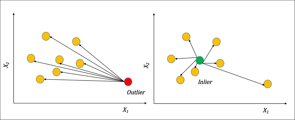
Figure 6: The ABOD method of distinguishing outliers from inliers
Given a point p, and any two points x and y, the angle between the two points and p is given by:
Measure of variance used as the ABOD score is given by:

The smaller the ABOD value, the smaller the measure of variance in the angle spectrum, and the larger the chance of the point being the outlier.
Another method that has been very useful in high dimensional data is using the Subspace Outlier Detection (SOD) approach (References [23]). The idea is to partition the high dimensional space such that there are an equal number of ranges, say ϕ, in each of the d dimensions. Then the Sparsity Coefficient for a cell C formed by picking a range in each of the d dimensions is measured as follows:

Here, n is the total number of data points and N(C) is the number of data points in cell C. Generally, the data points lying in cells with negative sparsity coefficient are considered outliers.
- The ABOD method is O(n3) with the number of data points and becomes impractical with larger datasets.
- The sparsity coefficient method in subspaces requires efficient search in lower dimension and the problem becomes NP-Hard and some form of evolutionary or heuristic based search is employed.
- The sparsity coefficient methods being NP-Hard can result in local optima.
In many domains there is a particular class or category of interest and the "rest" do not matter. Finding a boundary around this class of interest is the basic idea behind one-class SVM (References [26]). The basic assumption is that all the points of the positive class (class of interest) cluster together while the other class elements are spread around and we can find a tight hyper-sphere around the clustered instances. SVM, which has great theoretical foundations and applications in binary classifications is reformulated to solve one-class SVM. The following figure illustrates how a nonlinear boundary is simplified by using one-class SVM with slack so as to not overfit complex functions:

Figure 7: One-Class SVM for nonlinear boundaries
Data inputs are generally numeric features. Many SVMs can take nominal features and apply binary transformations to them. Also needed are: marking the class of interest, SVM hyper-parameters such as kernel choice, kernel parameters and cost parameter, among others. Output is a SVM model that can predict whether instances belong to the class of interest or not. This is different from scoring models, which we have seen previously.
The input is training instances {x1,x2…xn} with certain instances marked to be in class +1 and rest in -1.
The input to SVM also needs a kernel that does the transformation ϕ from input space to features space as ![]() using:
using:
Create a hyper-sphere that bounds the classes using SVM reformulated equation as:

Such that ![]() +
+![]() ,
, ![]()
R is the radius of the hyper-sphere with center c and ν ∈ (0,1] represents an upper bound on the fraction of the data that are outliers.
As in normal SVM, we perform optimization using quadratic programming is done to obtain the solution as the decision boundary.
- The key advantage to using one-class SVM—as is true of binary SVM—is the many theoretical guarantees in error and generalization bounds.
- High-dimensional data can be easily mapped in one-class SVM.
- Non-linear SVM with kernels can even find non-spherical shapes to bound the clusters of data.
- The training cost in space and memory increases as the size of the data increases.
- Parameter tuning, especially the kernel parameters and the cost parameter tuning with unlabeled data is a big challenge.
Measuring outliers in terms of labels, ranks, and scores is an area of active research. When the labels or the ground truth is known, the idea of evaluation becomes much easier as the outlier class is known and standard metrics can be employed. But when the ground truth is not known, the evaluation and validation methods are very subjective and there is no well-defined, rigorous statistical process.
In cases where the ground truth is known, the evaluation of outlier algorithms is basically the task of finding the best thresholds for outlier scores (scoring-based outliers).
The balance between reducing the false positives and improving true positives is the key concept and Precision-Recall curves (described in Chapter 2, Practical Approach to Real-World Supervised Learning) are used to find the best optimum threshold. Confidence score, predictions, and actual labels are used in supervised learning to plot PRCurves, and instead of confidence scores, outlier scores are ranked and used here. ROC curves and area under curves are also used in many applications to evaluate thresholds. Comparing two or more algorithms and selection of the best can also be done using area under curve metrics when the ground truth is known.
In most real-world cases, knowing the ground truth is very difficult, at least during the modeling task. Hawkins describes the evaluation method in this case at a very high level as "a sample containing outliers would show up such characteristics as large gaps between 'outlying' and 'inlying' observations and the deviation between outliers and the group of inliers, as measured on some suitably standardized scale".
The general technique used in evaluating outliers when the ground truth is not known is:
- Histogram of outlier scores: A visualization-based method, where outlier scores are grouped into predefined bins and users can select thresholds based on outlier counts, scores, and thresholds.
- Score normalization and distance functions: In this technique, some form of normalization is done to make sure all outlier algorithms that produce scores have the same ranges. Some form of distance or similarity or correlation based method is used to find commonality of outliers across different algorithms. The general intuition here is: the more the algorithms that weigh the data point as outlier, the higher the probability of that point actually being an outlier.