
The goal of feature relevance and selection is to find the features that are discriminating with respect to the target variable and help reduce the dimensions of the data [1,2,3]. This improves the model performance mainly by ameliorating the effects of the curse of dimensionality and by removing noise due to irrelevant features. By carefully evaluating models on the validation set with and without features removed, we can see the impact of feature relevance. Since the exhaustive search for k features involves 2k – 1 sets (consider all combinations of k features where each feature is either retained or removed, disregarding the degenerate case where none is present) the corresponding number of models that have to be evaluated can become prohibitive, so some form of heuristic search techniques are needed. The most common of these techniques are described next.
Some of the very common search techniques employed to find feature sets are:
- Forward or hill climbing: In this search, one feature is added at a time until the evaluation module outputs no further change in performance.
- Backward search: Starting from the whole set, one feature at a time is removed until no performance improvement occurs. Some applications interleave both forward and backward techniques to search for features.
- Evolutionary search: Various evolutionary techniques such as genetic algorithms can be used as a search mechanism and the evaluation metrics from either filter- or wrapper-based methods can be used as fitness criterion to guide the process.
At a high level, there are three basic methods to evaluate features.
This approach refers to the use of techniques without using machine learning algorithms for evaluation. The basic idea of the filter approach is to use a search technique to select a feature (or subset of features) and measure its importance using some statistical measure until a stopping criterion is reached.
This search is as simple as ranking each feature based on the statistical measure employed.
All information theoretic approaches use the concept of entropy mechanism at their core. The idea is that if the feature is randomly present in the dataset, there is maximum entropy, or, equivalently, the ability to compress or encode is low, and the feature may be irrelevant. On the other hand, if the distribution of the feature value is such some range of values are more prevalent in one class relative to the others, then the entropy is minimized and the feature is discriminating. Casting the problem in terms of entropy in this way requires some form of discretization to convert the numeric features into categories in order to compute the probabilities.
Consider a binary classification problem with training data DX. If Xi is the ith feature with v distinct categorical values such that DXi = {D1, D2… Dv}, then information or the entropy in feature Xi is:

Here, Info(Dj) is the entropy of the partition and is calculated as:

Here, p+(D) is the probability that the data in set D is in the positive class and p_(D) is the probability that it is in the negative class, in that sample. Information gain for the feature is calculated in terms of the overall information and information of the feature as
InfoGain(Xi) = Info(D) – Info(DXi)
For numeric features, the values are sorted in ascending order and split points between neighboring values are considered as distinct values.
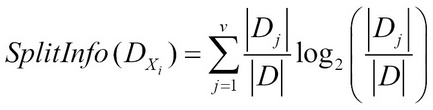
The greater the decrease in entropy, the higher the relevance of the feature. Information gain has problems when the feature has a large number of values; that is when Gain Ratio comes in handy. Gain Ratio corrects the information gain over large splits by introducing Split Information. Split Information for feature Xi and GainRatio is given by:

There are other impurity measures such as Gini Impurity Index (as described in the section on the Decision Tree algorithm) and Uncertainty-based measures to compute feature relevance.
Chi-Squared feature selection is one of the most common feature selection methods that has statistical hypothesis testing as its base. The null hypothesis is that the feature and the class variable are independent of each other. The numeric features are discretized so that all features have categorical values. The contingency table is calculated as follows:
|
Feature Values |
Class=P |
Class=N |
Sum over classes niP + niN |
|---|---|---|---|
|
X1 |
(n1P|µ1P) |
(n1N|µ1N) |
n1 |
|
…. |
… |
…. |
… |
|
Xm |
(nmP|µmP) |
(nmN|µmN) |
nm |
|
n*P |
n*P |
n |
Contingency Table 1: Showing feature values and class distribution for binary class.
In the preceding table, nij is a count of the number of features with value—after discretization—equal to xi and class value of j.
The value summations are:


Here n is number of data instances, j = P, N is the class value and i =1,2, … m indexes the different discretized values of the feature and the table has m – 1 degrees of freedom.
The Chi-Square Statistic is given by:

The Chi-Square value is compared to confidence level thresholds for testing significance. For example, for i = 2, the Chi-Squared value at threshold of 5% is 3.84; if our value is smaller than the table value of 3.83, then we know that the feature is interesting and the null hypothesis is rejected.
Most multivariate methods of feature selection have two goals:
- Reduce the redundancy between the feature and other selected features
- Maximize the relevance or correlation of the feature with the class label
The task of finding such subsets of features cannot be exhaustive as the process can have a large search space. Heuristic search methods such as backward search, forward search, hill-climbing, and genetic algorithms are typically used to find a subset of features. Two very well-known evaluation techniques for meeting the preceding goals are presented next.
In this technique, numeric features are often discretized—as done in univariate pre-processing—to get distinct categories of values.
For each subset S, the redundancy between two features Xi and Xj can be measured as:

Here, MI (Xi, Xj) = measure of mutual information between two features Xi and Xj. Relevance between feature Xi and class C can be measured as:

Also, the two goals can be combined to find the best feature subset using:

The basic idea is similar to the previous example; the overall merit of subset S is measured as:

Here, k is the total number of features, ![]() is the average feature class correlation and
is the average feature class correlation and ![]() is the average feature-feature inter correlation. The numerator gives the relevance factor while the denominator gives the redundancy factor and hence the goal of the search is to maximize the overall ratio or the Merit (S).
is the average feature-feature inter correlation. The numerator gives the relevance factor while the denominator gives the redundancy factor and hence the goal of the search is to maximize the overall ratio or the Merit (S).
There are other techniques such as Fast-Correlation-based feature selection that is based on the same principles, but with variations in computing the metrics. Readers can experiment with this and other techniques in Weka.
The advantage of the Filter approach is that its methods are independent of learning algorithms and hence one is freed from choosing the algorithms and parameters. They are also faster than wrapper-based approaches.
The search technique remains the same as discussed in the feature search approach; only the evaluation method changes. In the wrapper approach, a machine learning algorithm is used to evaluate the subset of features that are found to be discriminating based on various metrics. The machine learning algorithm used as the wrapper approach may be the same or different from the one used for modeling.
Most commonly, cross-validation is used in the learning algorithm. Performance metrics such as area under curve or F-score, obtained as an average on cross-validation, guide the search process. Since the cost of training and evaluating models is very high, we choose algorithms that have fast training speed, such as Linear Regression, linear SVM, or ones that are Decision Tree-based.
Some wrapper approaches have been very successful using specific algorithms such as Random Forest to measure feature relevance.
This approach does not require feature search techniques. Instead of performing feature selection as preprocessing, it is done in the machine learning algorithm itself. Rule Induction, Decision Trees, Random Forest, and so on, perform feature selection as part of the training algorithm. Some algorithms such as regression or SVM-based methods, known as shrinking methods, can add a regularization term in the model to overcome the impact of noisy features in the dataset. Ridge and lasso-based regularization are well-known techniques available in regressions to provide feature selection implicitly.
There are other techniques using unsupervised algorithms that will be discussed in Chapter 3, Unsupervised Machine Learning Techniques, that can be used effectively in a supervised setting too, for example, Principal Component Analysis (PCA).