
In Chapter 2, Practical Approach to Real-World Supervised Learning and Chapter 3, Unsupervised Machine Learning Techniques, we discussed two major groups of machine learning techniques which apply to opposite situations when it comes to the availability of labeled data—one where all target values are known and the other where none are. In contrast, the techniques in this chapter address the situation when we must analyze and learn from data that is a mix of a small portion with labels and a large number of unlabeled instances.
In speech and image recognition, a vast quantity of data is available, and in various forms. However, the cost of labeling or classifying all that data is costly and therefore, in practice, the proportion of speech or images that are classified to those that are not classified is very small. Similarly, in web text or document classification, there are an enormous number of documents on the World Wide Web but classifying them based on either topics or contexts requires domain experts—this makes the process complex and expensive. In this chapter, we will discuss two broad topics that cover the area of "learning from unlabeled data", namely Semi-Supervised Learning (SSL) and Active Learning. We will introduce each of the topics and discuss the taxonomy and algorithms associated with each as we did in previous chapters. Since the book emphasizes the practical approach, we will discuss tools and libraries available for each type of learning. We will then consider real-world case studies and demonstrate the techniques that are useful when applying the tools in practical situations.
Here is the list of topics that are covered in this chapter:
- Semi-Supervised Learning:
- Representation, notation, and assumptions
- Semi-Supervised Learning techniques:
- Self-training SSL
- Co-training SSL
- Cluster and label SSL
- Transductive graph label propagation
- Transductive SVM
- Case study in Semi-Supervised Learning
- Active Learning:
- Representation and notation
- Active Learning scenarios
- Active Learning approaches:
- Uncertainty sampling
- Least confident sampling
- Smallest margin sampling
- Label entropy sampling
- Version space sampling:
- Query by disagreement
- Query by committee
- Data distribution sampling:
- Expected model change
- Expected error reduction
- Variance reduction
- Density weighted methods
- Uncertainty sampling
- Case study in Active Learning
The idea behind semi-supervised learning is to learn from labeled and unlabeled data to improve the predictive power of the models. The notion is explained with a simple illustration, Figure 1, which shows that when a large amount of unlabeled data is available, for example, HTML documents on the web, the expert can classify a few of them into known categories such as sports, news, entertainment, and so on. This small set of labeled data together with the large unlabeled dataset can then be used by semi-supervised learning techniques to learn models. Thus, using the knowledge of both labeled and unlabeled data, the model can classify unseen documents in the future. In contrast, supervised learning uses labeled data only:


Figure 1. Semi-Supervised Learning process (bottom) contrasted with Supervised Learning (top) using classification of web documents as an example. The main difference is the amount of labeled data available for learning, highlighted by the qualifier "small" in the semi-supervised case.
As before, we will introduce the notation we use in this chapter. The dataset D consists of individual data instances represented as x, which is also represented as a set {x1, x2,…xn}, the set of data instances without labels. The labels associated with these data instances are {y1, y2, … yn}. The entire labeled dataset can be represented as paired elements in a set, as given by D = {(x1, y1), (x2,y2), … (xn, yn)} where xi ∈ ℝd. In semi-supervised learning, we divide the dataset D further into two sets U and L for unlabeled and labeled data respectively.
The labeled data ![]() consists of all labeled data with known outcomes {y1, y2, .. yl}. The unlabeled data
consists of all labeled data with known outcomes {y1, y2, .. yl}. The unlabeled data ![]() is the dataset where the outcomes are not known. |U| > |L| .
is the dataset where the outcomes are not known. |U| > |L| .
Inductive semi-supervised learning consists of a set of techniques, which, given the training set D with labeled data ![]() and unlabeled data
and unlabeled data ![]() , learns a model represented as
, learns a model represented as ![]() so that the model f can be a good predictor on unseen data beyond the training unlabeled data U. It "induces" a model that can be used just like supervised learning algorithms to predict on unseen instances.
so that the model f can be a good predictor on unseen data beyond the training unlabeled data U. It "induces" a model that can be used just like supervised learning algorithms to predict on unseen instances.
Transductive semi-supervised learning consists of a set of techniques, which, given the training set D, learns a model ![]() that makes predictions on unlabeled data alone. It is not required to perform on unseen future instances and hence is a simpler form of SSL than inductive based learning.
that makes predictions on unlabeled data alone. It is not required to perform on unseen future instances and hence is a simpler form of SSL than inductive based learning.
Some of the assumptions made in the semi-supervised learning algorithms that should hold true for these types of learning to be successful are noted in the following list. For SSL to work, one or more of these assumptions must be true:
- Semi-supervised smoothness: In simple terms, if two points are "close" in terms of density or distance, then their labels agree. Conversely, if two points are separated and in different density regions, then their labels need not agree.
- Cluster togetherness: If the data instances of classes tend to form a cluster, then the unlabeled data can aid the clustering algorithm to find better clusters.
- Manifold togetherness: In many real-world datasets, the high-dimensional data lies in a low-dimensional manifold, enabling learning algorithms to overcome the curse of dimensionality. If this is true in the given dataset, the unlabeled data also maps to the manifold and can improve the learning.
In this section, we will describe different SSL techniques, and some accompanying algorithms. We will use the same structure as in previous chapters and describe each method in three subsections: Inputs and outputs, How does it work?, and Advantages and limitations.
Self-training is the simplest form of SSL, where we perform a simple iterative process of imputing the data from the unlabeled set by applying the model learned from the labeled set (References [1]):

Figure 2. Self-training SSL in binary classification with some labeled data shown with blue rectangles and yellow circles. After various iterations, the unlabeled data gets mapped to the respective classes.
The input is training data with a small amount of labeled and a large amount of unlabeled data. A base classifier, either linear or non-linear, such as Naïve Bayes, KNN, Decision Tree, or other, is provided along with the hyper-parameters needed for each of the algorithms. The constraints on data types will be similar to the base learner. Stopping conditions such as maximum iterations reached or unlabeled data exhausted are choices that must be made as well. Often, we use base learners which give probabilities or ranks to the outputs. As output, this technique generates models that can be used for performing predictions on unseen datasets other than the unlabeled data provided.
The entire algorithm can be summarized as follows:
- While stopping criteria not reached:
-
Train the classifier model
 with labeled data L
 - Apply the classifier model f on unlabeled data U
- Choose k most confident predictions from U as set Lu
- Augment the labeled data with the k data points L = L ∪ Lu
-
Train the classifier model
- Repeat all the steps under 2.
In the abstract, self-training can be seen as an expectation maximization process applied to a semi-supervised setting. The process of training the classifier model is finding the parameter θ using MLE or MAP. Computing the labels using the learned model is similar to the EXPECTATION step where ![]() is estimating the label from U given the parameter θ. The iterative next step of learning the model with augmented labels is akin to the MAXIMIZATION step where the new parameter is tuned to θ'.
is estimating the label from U given the parameter θ. The iterative next step of learning the model with augmented labels is akin to the MAXIMIZATION step where the new parameter is tuned to θ'.
Co-training based SSL involves learning from two different "views" of the same data. It is a special case of multi-view SS (References [2]). Each view can be considered as a feature set of the point capturing some domain knowledge and is orthogonal to the other view. For example, a web documents dataset can be considered to have two views: one view is features representing the text and the other view is features representing hyperlinks to other documents. The assumption is that there is enough data for each view and learning from each view improves the overall labeling process. In datasets where such partitions of features are not possible, splitting features randomly into disjoint sets forms the views.
Input is training data with a few labeled and a large number of unlabeled data. In addition to providing the data points, there are feature sets corresponding to each view and the assumption is that these feature sets are not overlapping and solve different classification problems. A base classifier, linear or non-linear, such as Naïve Bayes, KNN, Decision Tree, or any other, is selected along with the hyper-parameters needed for each of the algorithms. As output, this method generates models that can be used for performing predictions on unseen datasets other than the unlabeled data provided.
We will demonstrate the algorithm using two views of the data:
-
Initialize the data as
 labeled and
  unlabeled. Each data point has two views x = [x1,x2] and L = [L1,L2].
- While stopping criteria not reached:
-
Train the classifier models
 and
and  with labeled data L1 and L2 respectively.
- Apply the classifier models f1 and f2 on unlabeled data U using their own features.
- Choose k the most confident predictions from U, applying f1 and f2 as set Lu1 and Lu2 respectively.
- Augment the labeled data with the k data points L1 = L1 ∪ Lu1 and L2 = L2 ∪ Lu2
-
Train the classifier models
- Repeat all the steps under 2.
The advantages and limitations are:
This technique, like self-training, is quiet generic and applicable to domains and datasets where the clustering supposition mentioned in the assumptions section holds true (References [3]).
Input is training data with a few labeled and a large number of unlabeled instances. A clustering algorithm and its parameters along with a classification algorithm with its parameters constitute additional inputs. The technique generates a classification model that can help predict the classes of unseen data.
The abstract algorithm can be given as:
-
Initialize data as labeled and unlabeled.
- Cluster the entire data, both labeled and unlabeled using the clustering algorithm.
- For each cluster let S be the set of labeled instances drawn from set L.
- Learn a supervised model from S, fs = Ls.
- Apply the model fs and classify unlabeled instances for each cluster using the preceding model.
-
Since all the unlabeled instances get assigned a label by the preceding process, a supervised classification model is run on the entire set.

Figure 3. Clustering and label SSL – clustering followed by classification
The key idea behind graph-based methods is to represent every instance in the dataset, labeled and unlabeled, as a node and compute the edges as some form of "similarity" between them. Known labels are used to propagate labels in the unlabeled data using the basic concepts of label smoothness as discussed in the assumptions section, that is, similar data points will lie "close" o each other graphically (References [4]).
Figure 4 shows how the similarity indicated by the thickness of the arrow from the first data point to the last varies when the handwritten digit pattern changes. Knowing the first label, the label propagation can effectively label the next three digits due to the similarity in features while the last digit, though labeled the same, has a lower similarity as compared to the first three.

Figure 4. Transductive graph label propagation – classification of hand-written digits. Leftmost and rightmost images are labeled, others are unlabeled. Arrow thickness is a visual measure of similarity to labeled digit "2" on the left.
Input is training data with a few labeled and a large number of unlabeled data. The graph weighting or similarity computing method, such as k-nearest weighting, Gaussian decaying distance, or ϵ-radius method is chosen. Output is the labeled set for the entire data; it generally doesn't build inductive models like the algorithms seen previously.
The general label propagation method follows:
- Build a graph g = (V,E) where:
- Vertices V = {1, 2…n} correspond to data belonging to both labeled set L and unlabeled set U.
- Edges E are weight matrices W, such that Wi,j represents similarity in some form between two data points xi, xj.
-
Compute the diagonal degree matrix D by
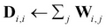 .
.
-
Assume the labeled set is binary and has
 . Initialize the labels of all unlabeled data to be 0.
- Iterate at t = 0:

 (reset the labels of labeled instances back to the original)
-
Go back to step 4, until convergence

-
Label the unlabeled points using the convergence labels .
There are many variations based on similarity, optimization selected in iterations, and so on.
The advantages and limitations are:
- The graph-based semi-supervised learning methods are costly in terms of computations—generally O(n3) where n is the number of instances. Though speeding and caching techniques help, the computational cost over large data makes it infeasible in many real-world data situations.
- The transductive nature makes it difficult for practical purposes where models need to be induced for unseen data. There are extensions such as Harmonic Mixtures, and so on, which address these concerns.
Transductive SVM is one of the oldest and most popular transductive semi-supervised learnig methods, introduced by Vapnik (References [5]). The key principle is that unlabeled data along with labeled data can help find the decision boundary using concepts of large margins. The underlying principle is that the decision boundaries normally don't lie in high density regions!
Input is training data with few labeled and a large number of unlabeled data. Input has to be numeric features for TSVM computations. The choice of kernels, kernel parameters, and cost factors, which are all SVM-based parameters, are also input variables. The output is labels for the unlabeled dataset.
Generally, SVM works as an optimization problem in the labeled hard boundary SVM formulated in terms of weight vector w and the bias b  subject to
 ![]()
-
Initialize the data as labeled and unlabeled.
- In TSVM, the equation is modified as follows:
This is subject to the following condition:


This is exactly like inductive SVM but using only labeled data. When we constrain the unlabeled data to conform to the side of the hyperplane of labeled data in order to maximize the margin, it results in unlabeled data being labeled with maximum margin separation! By adding the penalty factor to the constraints or replacing the dot product in the input space with kernels as in inductive SVM, complex non-linear noisy datasets can be labeled from unlabeled data.
Figure 5 illustrates the concept of TSVM in comparison with inductive SVM run on labeled data only and why TSVM can find better decision boundaries using the unlabeled datasets. The unlabeled datasets on either side of hyperplane are closer to their respective classes, thus helping find better margin separators.

Figure 5. Transductive SVM
For this case study, we use another well-studied dataset from the UCI Repository, the Wisconsin Breast Cancer dataset. In the first part of the experiment, we demonstrate how to apply the Transductive SVM technique of semi-supervised learning using the open-source library called JKernelMachines. We choose the SVMLight algorithm and a Gaussian kernel for this technique.
In the second part, we use KEEL, a GUI-based framework and compare results from several evolutionary learning based algorithms using the UCI Breast Cancer dataset. The tools, methodology, and evaluation measures are described in the following subsections.
The two open source Java tools used in the semi-supervised learning case study are JKernelMachines, a Transductive SVM, and KEEL, a GUI-based tool that uses evolutionary algorithms for learning.
Note
JKernelMachines (Transductive SVM)
JKernelMachines is a pure Java library that provides an efficient framework for using and rapidly developing specialized kernels. Kernels are similarity functions used in SVMs. JKernelMachines provides kernel implementations defined on structured data in addition to standard kernels on vector data such as Linear and Gaussian. In particular, it offers a combination of kernels, kernels defined over lists, and kernels with various caching strategies. The library also contains SVM optimization algorithm implementations including LaSVM and One-Class SVM using SMO. The creators of the library report that the results of JKernelMachines on some common UCI repository datasets are comparable to or better than the Weka library.
The example of loading data and running Transductive SVM using JKernelMachines is given here:
try {
//load the labeled training data
List<TrainingSample<double[]>> labeledTraining = ArffImporter.importFromFile("resources/breast-labeled.arff");
//load the unlabeled data
List<TrainingSample<double[]>> unlabeledData =ArffImporter.importFromFile("resources/breast-unlabeled.arff");
//create a kernel with Gaussian and gamma set to 1.0
DoubleGaussL2 k = new DoubleGaussL2(1.0);
//create transductive SVM with SVM light
S3VMLight<double[]> svm = new S3VMLight<double[]>(k);
//send the training labeled and unlabeled data
svm.train(labeledTraining, unlabeledData);
} catch (IOException e) {
	e.printStackTrace();
}
In the second approach, we use KEEL with the same dataset.
Note
KEEL
KEEL (Knowledge Extraction based on Evolutionary Learning) is a non-commercial (GPLv3) Java tool with GUI which enables users to analyze the behavior of evolutionary learning for a variety of data mining problems, including regression, classification, and unsupervised learning. It relieves users from the burden of programming sophisticated evolutionary algorithms and allows them to focus on new learning models created using the toolkit. KEEL is intended to meet the needs of researchers as well as students.
KEEL contains algorithms for data preprocessing and post-processing as well as statistical libraries, and a Knowledge Extraction Algorithms Library which incorporates multiple evolutionary learning algorithms with classical learning techniques.
The GUI wizard included in the tool offers different functional components for each stage of the pipeline, including:
- Data management: Import, export of data, data transformation, visualization, and so on
- Experiment design: Selection of classifier, estimator, unsupervised techniques, validation method, and so on
- SSL experiments: Transductive and inductive classification (see image of off-line method for SSL experiment design in this section)
- Statistical analysis: This provides tests for pair-wise and multiple comparisons, parametric, and non-parametric procedures.
For more info, visit http://sci2s.ugr.es/keel/ and http://sci2s.ugr.es/keel/pdf/keel/articulo/Alcalaetal-SoftComputing-Keel1.0.pdf.

Figure 6: KEEL – wizard-based graphical interface
Breast cancer is the top cancer in women worldwide and is increasing particularly in developing countries where the majority of cases are diagnosed in late stages. Examination of tumor mass using a non-surgical procedure is an inexpensive and preventative measure for early detection of the disease.
In this case-study, a marked dataset from such a procedure is used and the goal is to classify the breast cancer data into Malignant and Benign using multiple SSL techniques.
To illustrate the techniques learned in this chapter so far, we will use SSL to classify. Whereas the dataset contains labels for all the examples, in order to treat this as a problem where we can apply SSL, we will consider a fraction of the data to be unlabeled. In fact, we run multiple experiments using different fractions of unlabeled data for comparison. The different base learners used are classification algorithms familiar to us from previous chapters.
This dataset was collected by the University of Wisconsin Hospitals, Madison. The dataset is available in Weka AARF format. The data is not partitioned into training, validation and test.
In the experiments, we present results for 10-fold cross-validation. For comparison, four runs were performed each using a different fraction of labeled data—10%, 20%, 30%, and 40%.
A numeric sample code number was added to each example as a unique identifier. The categorical values Malignant and Benign, for the class attribute, were replaced by the numeric values 4 and 2 respectively.
The Breast Cancer Dataset Wisconsin (Original) is available from the UCI Machine Learning Repository at: https://archive.ics.uci.edu/ml/datasets/Breast+Cancer+Wisconsin+(Original).
This database was originally obtained from the University of Wisconsin Hospitals, Madison from Dr. William H. Wolberg. The dataset was created by Dr. Wolberg for the diagnosis and prognosis of breast tumors. The data is based exclusively on measurements involving the Fine Needle Aspirate (FNA) test. In this test, fluid from a breast mass is extracted using a small-gauge needle and then visually examined under a microscope.
A total of 699 instances with nine numeric attributes and a binary class (malignant/benign) constitute the dataset. The percentage of missing values is 0.2%. There are 65.5% malignant and 34.5% benign cases in the dataset. The feature names and range of valid values are listed in the following table:
|
Num. |
Feature Name |
Domain |
|---|---|---|
|
1 |
Sample code number |
id number |
|
2 |
Clump Thickness |
1 - 10 |
|
3 |
Uniformity of Cell Size |
1 - 10 |
|
4 |
Uniformity of Cell Shape |
1 - 10 |
|
5 |
Marginal Adhesion |
1 - 10 |
|
6 |
Single Epithelial Cell Size |
1 - 10 |
|
7 |
Bare Nuclei |
1 - 10 |
|
8 |
Bland Chromatin |
1 - 10 |
|
9 |
Normal Nucleoli |
1 - 10 |
|
10 |
Mitoses |
1 - 10 |
|
11 |
Class |
2 for benign, 4 for malignant |
Summary statistics by feature appear in Table 1.
|
Clump Thickness |
Cell Size Unifor-mity |
Cell Shape Unifor-mity |
Marginal Adhesion |
Single Epi Cell Size |
Bare Nuclei |
Bland Chromatin |
Normal Nucleoli |
Mitoses | |
|---|---|---|---|---|---|---|---|---|---|
|
mean |
4.418 |
3.134 |
3.207 |
2.807 |
3.216 |
3.545 |
3.438 |
2.867 |
1.589 |
|
std |
2.816 |
3.051 |
2.972 |
2.855 |
2.214 |
3.644 |
2.438 |
3.054 |
1.715 |
|
min |
1 |
1 |
1 |
1 |
1 |
1 |
1 |
1 |
1 |
|
25% |
2 |
1 |
1 |
1 |
2 |
2 |
1 |
1 | |
|
50% |
4 |
1 |
1 |
1 |
2 |
3 |
1 |
1 | |
|
75% |
6 |
5 |
5 |
4 |
4 |
5 |
4 |
1 | |
|
max |
10 |
10 |
10 |
10 |
10 |
10 |
10 |
10 |
10 |
Table 1. Features summary
Two SSL algorithms were selected for the experiments—self-training and co-training. In addition, four classification methods were chosen as base learners—Naïve Bayes, C4.5, K-NN, and SMO. Further, each experiment was run using four different partitions of labeled and unlabeled data (10%, 20%, 30%, and 40% labeled).
The hyper-parameters for the algorithms and base classifiers are given in Table 2. You can see the accuracy across the different runs corresponding to four partitions of labeled and unlabeled data for the two SSL algorithms.
Finally, we give the performance results for each experiment for the case of 40% labeled. Performance metrics provided are Accuracy and the Kappa statistic with standard deviations.
|
Method |
Parameters |
|---|---|
|
Self-Training |
MAX_ITER = 40 |
|
Co-Training |
MAX_ITER = 40, Initial Unlabeled Pool=75 |
|
KNN |
K = 3, Euclidean distance |
|
C4.5 |
pruned tree, confidence = 0.25, 2 examples per leaf |
|
NB |
No parameters specified |
|
SMO |
C = 1.0, Tolerance Parameter = 0.001, Epsilon= 1.0E-12, Kernel Type = Polynomial, Polynomial degree = 1, Fit logistic models = true |
Table 2. Base classifier hyper-parameters for self-training and co-training
|
SSL Algorithm |
10% |
20% |
30% |
40% |
|
Self-Training C 4.5 |
0.9 |
0.93 |
0.94 |
0.947 |
|
Co-Training SMO |
0.959 |
0.949 |
0.962 |
0.959 |
Table 3. Model accuracy for samples with varying fraction of labeled examples
|
Algorithm |
Accuracy (no unlabeled) |
|---|---|
|
C4.5 10-fold CV |
0.947 |
|
SMO 10 fold CV |
0.967 |
|
10 fold CV Wisconsin 40% Labeled Data | ||||
|
Self-Training (kNN) |
Accuracy |
0.9623 (1) |
Kappa |
0.9170 (2) |
|
Std Dev |
0.0329 |
Std Dev |
0.0714 | |
|
Self-Training (C45) |
Accuracy |
0.9606 (3) |
Kappa |
0.9144 |
|
Std Dev |
0.0241 |
Std Dev |
0.0511 | |
|
Self-Training (NB) |
Accuracy |
0.9547 |
Kappa |
0.9036 |
|
Std Dev |
0.0252 |
Std Dev |
0.0533 | |
|
Self-Training (SMO) |
Accuracy |
0.9547 |
Kappa |
0.9035 |
|
Std Dev |
0.0208 |
Std Dev |
0.0435 | |
|
Co-Training (NN) |
Accuracy |
0.9492 |
Kappa |
0.8869 |
|
Std Dev |
0.0403 |
Std Dev |
0.0893 | |
|
Co-Training (C45) |
Accuracy |
0.9417 |
Kappa |
0.8733 |
|
Std Dev |
0.0230 |
Std Dev |
0.0480 | |
|
Co-Training (NB) |
Accuracy |
0.9622 (2) |
Kappa |
0.9193 (1) |
|
Std Dev |
0.0290 |
Std Dev |
0.0614 | |
|
Co-Training (SMO) |
Accuracy |
0.9592 |
Kappa |
0.9128 (3) |
|
Std Dev |
0.0274 |
Std Dev |
0.0580 | |
Table 4. Model performance comparison using 40% labeled examples. The top ranking performers in each category are shown in parentheses.
With 40% of labeled data, semi-supervised self-training with C4.5 achieves the same result as 100% of labeled data with just C4.5. This shows the strength of semi-supervised learning when the data is sparsely labeled.
SMO with polynomial kernel, with 30-40% data comes close to the 100% data but not as good as C4.5.
Self-training and co-training with four classifiers on 40% labeled training data shows
- KNN as base classifier and self-training has the highest accuracy (0.9623) which indicates the non-linear boundary of the data. Co-training with Naïve Bayes comes very close.
- Self-training with classifiers such as linear Naïve Bayes, non-linear C4.5 and highly non-linear KNN shows steady improvements in accuracy: 0.9547, 0.9606, 0.9623, which again shows that using self-training but choosing the right underlying classifier for the problem is very important.
- Co-training with Naive Bayes has highest Kappa statistic (0.9193) and almost similar accuracy as KNN with self-training. The independence relationship between features—hence breaking the feature sets into orthogonal feature sets and using them for classifiers—improves the learning.