Deep learning includes architectures and techniques for supervised and unsupervised learning with the capacity to internalize the abstract structure of high-dimensional data using networks composed of building blocks to create discriminative or generative models. These techniques have proved enormously successful in recent years and any reader interested in mastering them must become familiar with the basic building blocks of deep learning first and understand the various types of networks in use by practitioners. Hands-on experience building and tuning deep neural networks is invaluable if you intend to get a deeper understanding of the subject. Deep learning, in various domains such as image classification and text learning, incorporates feature generation in its structures thus making the task of mining the features redundant in many applications. The following sections provide a guide to the concepts, building blocks, techniques for composing architectures, and training deep networks.
In the following sections, we introduce the most important components used in deep learning, including Restricted Boltzmann machines, Autoencoders, and Denoising Autoencoders, how they work, and their advantages and limitations.
The Reclin function is given by the equation:
g(a) = reclin (a) = max (0, a)
It can be seen as having a lower bound of 0 and no upper bound, strictly increasing, and a positive transformation function that just does linear transformation of positives.
It is easier to see that the rectified linear unit or ReLu has a derivative of 1 or identity for values greater than 0. This acts as a significant benefit as the derivatives are not squashed and do not have diminishing values when chained. One of the issues with ReLu is that the value is 0 for negative inputs and the corresponding neurons act as "dead", especially when a large negative value is learned for the bias term. ReLu cannot recover from this as the input and derivative are both 0. This is generally solved by having a "leaky ReLu". These functions have a small value for negative inputs and are given by 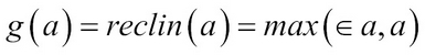 where ? = 0.01, typically.
Restricted Boltzmann Machines (RBM) is an unsupervised learning neural network (References [11]). The idea of RBM is to extract "more meaningful features" from labeled or unlabeled data. It is also meant to "learn" from the large quantity of unlabeled data available in many domains when getting access to labeled data is costly or difficult.
In its basic form RBM assumes inputs to be binary values 0 or 1 in each dimension. RBMs are undirected graphical models having two layers, a visible layer represented as x and a hidden layer h, and connections W.
RBM defines a distribution over the visible layer that involves the latent variables from the hidden layer. First an energy function is defined to capture the relationship between the visible and the hidden layers in vector form as:

In scalar form the energy function can be defined as:

The probability of the distribution is given by ![]() where Z is called the "partitioning function", which is an enumeration over all the values of x and h, which are binary, resulting in exponential terms and thus making it intractable!
where Z is called the "partitioning function", which is an enumeration over all the values of x and h, which are binary, resulting in exponential terms and thus making it intractable!

Figure 6: Connection between the visible layer and hidden layer.
The Markov network view of the same in scalar form can be represented using all the pairwise factors, as shown in the following figure. This also makes it clear why it is called a "restricted" Boltzmann machine as there is no connection among units within a given hidden layer or in the visible layers:


Figure 7: Input and hidden layers as scalars
We have seen that the whole probability distribution function ![]() is intractable. We will now derive the basic conditional probability distributions for x, h.
is intractable. We will now derive the basic conditional probability distributions for x, h.
Although computing the whole p(x, h) is intractable, the conditional distribution of p(x|h) or p(h|x) can be easily defined and shown to be a Bernoulli distribution and tractable:


Similarly, being symmetric and undirected:


RBMs are trained using the optimization objective of minimizing the average negative log-likelihood over the entire training data. This can be represented as:
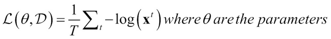
The optimization is carried out by using stochastic gradient descent:

The term  is called the "positive phase" and the term
 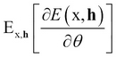 is called the "negative phase" because of how they affect the probability distributions—the positive phase, because it increases the probability of training data by reducing the free energy, and the negative phase, as it decreases the probability of samples generated by the model.
It has been shown that the overall gradient is difficult to compute analytically because of the "negative phase", as it is computing the expectation over all possible configurations of the input data under the distribution formed by the model and making it intractable!
To make the computation tractable, estimation is carried out using a fixed number of model samples and they are referred to as "negative particles" denoted by N.
The gradient can be now written as the approximation:

Where particles ![]() are sampled using some sampling techniques such as the Monte Carlo method.
are sampled using some sampling techniques such as the Monte Carlo method.
Gibbs sampling is often the technique used to generate samples and learn the probability of p(x,h) in terms of p(x|h) and p (h|x), which are relatively easy to compute, as shown previously.
Gibbs sampling for joint sampling of N random variables ![]() is done using N sampling sub-steps of the form
is done using N sampling sub-steps of the form ![]() where S
-i contains samples up to and excluding step S
i. Graphically, this can be shown as follows:
where S
-i contains samples up to and excluding step S
i. Graphically, this can be shown as follows:

Figure 8: Graphical representation of sampling done between hidden and input layers.
As ![]() it can be shown that the sampling represents the actual distribution p(x,h).
it can be shown that the sampling represents the actual distribution p(x,h).
Contrastive divergence (CD) is a trick used to expedite the Gibbs sampling process described previously so it stops at step k of the process rather than continuing for a long time to guarantee convergence. It has been seen that even k=1 is reasonable and gives good performance (References [10]).
These are the inputs to the algorithm:
- Training dataset
- Number of steps for Gibbs sampling, k
- Learning rate a
- The output is the set of updated parameters


Persistent contrastive divergence is another trick used to compute the joint probability p(x,h). In this method, there is a single chain that does not reinitialize after every observed sample to find the negative particle ![]() . It persists its state and parameters are updated just through running these k states by using the particle from the previous step.
. It persists its state and parameters are updated just through running these k states by using the particle from the previous step.
An autoencoder is another form of unsupervised learning technique in neural networks. It is very similar to the feed-forward neural network described at the start with the only difference being it doesn't generate a class at output, but tries to replicate the input at the output layer (References [12 and 23]). The goal is to have hidden layer(s) capture the latent or hidden information of the input as features that can be useful in unsupervised or supervised learning.
A single hidden layer example of an Autoencoder is shown in the following figure:

Figure 9: Autoencoder flow between layers
The input layer and the output layer have the same number of neurons similar as feed-forward, corresponding to the input vector, x. Each hidden layer can have greater, equal, or fewer neurons than the input or output layer and an activation function that does a non-linear transformation of the signal. It can be seen as using the unsupervised or latent hidden structure to "compress" the data effectively.
The encoder or input transformation of the data by the hidden layer is given by:

And the decoder or output transformation of the data by the output layer is given by:

Generally, a sigmoid function with linear transformation of signals as described in the neural network section is popularly used in the layers:
 and
and ![]() )
)
The job of the loss function is to reduce the training error as before so that an optimization process such as a stochastic gradient function can be used.
In the case of binary valued input, the loss function is generally the average cross-entropy given by:

It can be easily verified that, when the input signal and output signal match either 0 or 1, the error is 0. Similarly, for real-valued input, a squared error is used:

The gradient of the loss function that is needed for the stochastic gradient procedure is similar to the feed-forward neural network and can be shown through derivation for both real-valued and binary as follows:

Parameter gradients are obtained by back-propagating the ![]() exactly as in the neural network.
exactly as in the neural network.
Autoencoders have some known drawbacks that have been addressed by specialized architectures that we will discuss in the sections to follow. These limitations are:
When the size of the Autoencoder is equal to the number of neurons in the input, there is a chance that the weights learned by the Autoencoders are just the identity vectors and that the whole representation simply passes on the inputs exactly as outputs with zero loss. Thus, they emulate "rote learning" or "memorization" without any generalization.
When the size of the Autoencoder is greater than the number of neurons in the input, the configuration is called an "overcomplete" hidden layer and can have similar problems to the ones mentioned previously. Some of the units can be turned off and others can become identity making it just the copy unit.
When the size of the Autoencoder is less than the number of neurons in the input, known as "undercomplete", the latent structure in the data or important hidden components can be discovered.
As mentioned previously, when the Autoencoder has a hidden layer size greater than or equal to that of the input, it is not guaranteed to learn the weights and can become simply a unit switch to copy input to output. This issue is addressed by the Denoising Autoencoder. Here there is another layer added between input and the hidden layer. This layer adds some noise to the input using either a well-known distribution ![]() or using stochastic noise such as turning a bit to 0 in binary input. This "noisy" input then goes through learning from the hidden layer to the output layer exactly like the Autoencoder. The loss function of the Denoising Autoencoder compares the output with the actual input. Thus, the added noise and the larger hidden layer enable either learning latent structures or adding/removing redundancy to produce the exact signal at the output. This architecture—where non-zero features at the noisy layer generate features at the hidden layer that are themselves transformed by the activation layer as the signal advances forward—lends a robustness and implicit structure to the learning press (References [15]).
or using stochastic noise such as turning a bit to 0 in binary input. This "noisy" input then goes through learning from the hidden layer to the output layer exactly like the Autoencoder. The loss function of the Denoising Autoencoder compares the output with the actual input. Thus, the added noise and the larger hidden layer enable either learning latent structures or adding/removing redundancy to produce the exact signal at the output. This architecture—where non-zero features at the noisy layer generate features at the hidden layer that are themselves transformed by the activation layer as the signal advances forward—lends a robustness and implicit structure to the learning press (References [15]).

Figure 10: Denoising Autoencoder
As we discussed in the issues section on neural networks, the issue with over-training arises especially in deep learning as the number of layers, and hence parameters, is large. One way to account for over-fitting is to do data-specific regularization. In this section, we will describe the "unsupervised pre-training" method done in the hidden layers to overcome the issue of over-fitting. Note that this is generally the "initialization process" used in many deep learning algorithms.
The algorithm of unsupervised pre-training works in a layer-wise greedy fashion. As shown in the following figure, one layer of a visible and hidden structure is considered at a given time. The weights of this layer are learned for a few iterations using unsupervised techniques such as RBM, described previously. The output of the hidden layer is then used as a "visible" or "input" layer and the training proceeds to the next, and so on.
Each learning of layers can be thought of as a "feature extraction or feature generation" process. The real data inputs when transformed form higher-level features at a given layer and then are further combined to form much higher-level features, and so on.

Figure 11: Layer wise incremental learning through unsupervised learning.
Once all the hidden layer parameters are learned in pre-training using unsupervised techniques as described previously, a supervised fine-tuning process follows. In the supervised fine-tuning process, a final output layer is added and, just like in a neural network, training is done with forward and backward propagation. The idea is that most weights or parameters are almost fully tuned and only need a small change for producing a discriminative class mapping at the output.

Figure 12: Final tuning or supervised learning.
A deep feed-forward neural network involves using the stages pre-training, and fine-tuning.
Depending on the unsupervised learning technique used—RBM, Autoencoders, or Denoising Autoencoders—different algorithms are formed: Stacked RBM, Stacked Autoencoders, and Stacked Denoising Autoencoders, respectively.
Given an architecture for the deep feed-forward neural net, these are the inputs for training the network:
The generalized learning/training algorithm for all three is given as follows:
- For layers l=1 to L (Pre-Training):
-
Dataset without Labels

- Perform Step-wise Layer Unsupervised Learning (RBM, Autoencoders, or Denoising Autoencoders)
- Finalize the parameters Wl, bl from the preceding step
-
Dataset without Labels
- For the output layer (L+1) perform random initialization of parameters WL+1, bL +1.
- For layers l=1 to L+1 (Fine-Tuning):

Deep Autoencoders have many layers of hidden units, which shrink to a very small dimension and then symmetrically grow to the input size.

Figure 13: Deep Autoencoders
The idea behind Deep Autoencoders is to create features that capture latent complex structures of input using deep networks and at the same time overcome the issue of gradients and underfitting due to the deep structure. It was shown that this methodology generated better features and performed better than PCA on many datasets (References [13]).
Deep Autoencoders use the concept of pre-training, encoders/decoders, and fine-tuning to perform unsupervised learning:
In the pre-training phase, the RBM methodology is used to learn greedy stepwise parameters of the encoders, as shown in the following figure, for initialization:

Figure 14: Stepwise learning in RBM
In the unfolding phase the same parameters are symmetrically applied to the decoder network for initialization.
Finally, fine-tuning backpropagation is used to adjust the parameters across the entire network.
Deep Belief Networks (DBNs) are the origin of the concept of unsupervised pre-training (References [9]). Unsupervised pre-training originated from DBNs and then was found to be equally useful and effective in the feed-forward supervised deep networks.
Deep belief networks are not supervised feed-forward networks, but a generative model to generate data samples.
The input layer is the instance of data, represented by one neuron for each input feature. The output of a DBN is a reconstruction of the input from a hierarchy of learned features of increasingly greater abstraction.
How a DBN learns the joint distribution of the input data is explained here using a three-layer DBN architecture as an example.

Figure 15: Deep belief network
The three-hidden-layered DBN as shown has a first layer of undirected RBM connected to a two-layered Bayesian network. The Bayesian network with a sigmoid activation function is called a sigmoid Bayesian network (SBN).
The goal of a generative model is to learn the joint distribution as given by p(x,h(1),h(2),h(3))
p(x,h(1),h(2),h(3)) = p(h2),h(3))p(h(1)|h(2)) p(x|h(1))
RBM computation as seen before gives us:

The Bayesian Network in the next two layers is:


For binary data:

Another technique used to overcome the "overfitting" issues mentioned in deep neural networks is using the dropout technique to learn the parameters. In the next sections, we will define, illustrate, and explain how deep learning with dropouts works.
The idea behind dropouts is to "cripple" the deep neural network structure by stochastically removing some of the hidden units as shown in the following figure after the parameters are learned. The units are set to 0 with the dropout probability generally set as p=0.5
The idea is similar to adding noise to the input, but done in all the hidden layers. When certain features (or a combination of features) are removed stochastically, the neural network has to learn latent features in a more robust way, without the interdependence of some features.

Figure 16: Deep learning with dropout indicated by dropping certain units with dark shading.
Each hidden layer is represented by hk(x) where k is the layer. The pre-activation for layer 0<k<l is given by:

The hidden layer activation for 1< k < l. Binary masks are represented by mk at each hidden layer:

The final output layer activation is:

For training with dropouts, inputs are:
- Network architecture
- Training dataset
- Dropout probability p (typically 0.5)
The output is a trained deep neural net that can be applied for predictive use.
The backward propagation learning of weights and biases from the output loss function using gradients is very similar to traditional neural network learning. The only difference is that masks are applied appropriately as follows:
Compute the output gradient before activation:

For hidden layers k=l+1 to 1:
Compute the gradient of hidden layer parameters:


hk-1 computation has taken into account the binary mask mk-1 applied.
Compute the gradient of the hidden layer below the current:

Compute the gradient of the layer below before activation:

When testing the model, we cannot use the binary mask as it is stochastic; the "expectation" value of the mask is used. If the dropout probability is p=0.5, the same value 0.5 is used as the expectation for the unit at test or model application time.
Sparse coding is another neural network used for unsupervised learning and feature generation (References [22]). It works on the principle of finding latent structures in high dimensions that capture the patterns, thus performing feature extraction in addition to unsupervised learning.
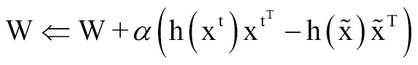
Formally, for every input x(t) a latent representation h(t) is learned, which has a sparse representation (most values are 0 in the vector). This is done by optimization using the following objective function:

Where the first term 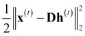 is to control the reconstruction error and the second term, which uses a regularizer ?, is for sparsity control. The matrix D is also known as a Dictionary as it has equivalence to words in a dictionary and h(t) is similar to word frequency; together they capture the impact of words in extracting patterns when performing text mining.
Convolutional Neural Networks or CNNs have become prominent and are widely used in the computer vision domain. Computer vision involves processing images/videos for capturing knowledge and patterns. Annotating images, classifying images/videos, correcting them, story-telling or describing images, and so on, are some of the broad applications in computer visi [16].
Computer vision problems most generally have to deal with unstructured data that can be described as:
Inputs that are 2D images with single or multiple color channels or 3D videos that are high-dimensional vectors.
The features in these 2D or 3D representations have a well-known spatial topology, a hierarchical structure, and some repetitive elements that can be exploited.
The images/videos have a large number of transformations or variants based on factors such as illumination, noise, and so on. The same person or car can look different based on several factors.
Next, we will describe some building blocks used in CNNs. We will use simple images such as the letter X of the alphabet to explain the concept and mathematics involved. For example, even though the same character X is represented in different ways in the following figure due to translation, scaling, or distortion, the human eye can easily read it as X, but it becomes tricky for the computer to see the pattern. The images are shown with the author's permission (References [19]):

Figure 17: Image of character X represented in different ways.
The following figure illustrates how a simple grayscale image of X has common features such as a diagonal from top left, a diagonal from top right, and left and right intersecting diagonals repeated and combined to form a larger X:
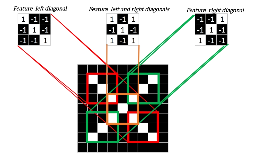
Figure 18: Common features represented in the image of character X.
This is the simple concept of dividing the whole image into "patches" or "recipient fields" and giving each patch to the hidden layers. As shown in the figure, instead of 9 X 9 pixels of the complete sample image, a 3 X 3 patch of pixels from the top left goes to the first hidden unit, the overlapping second patch goes to second, and so on.
Since the fully connected hidden layer would have a huge number of parameters, having smaller patches completely reduces the parameter or high-dimensional space problem!
Figure 19: Concept of patches on the whole image.
The concept of parameter sharing is to construct a weight matrix that can be reused over different patches or recipient fields as constructed in the preceding figure in the local sharing. As shown in the following figure, the Feature map with same parameters W1,1 and W1,4 creates two different feature maps, Feature Map 1 and 4, both capturing the same features, that is, diagonal edges on either side. Thus, feature maps capture "similar regions" in the images and further reduce the dimensionality of the input space.

We will explain the steps in discrete convolution, taking a simple contrived example with simplified mathematics to illustrate the operation.
Suppose the kernel representing the diagonal feature is scanned over the entire image as a patch of 3 X 3. If this kernel lands on the self-same feature in the input image and we have to compute the center value through what we call the convolution operator, we get the exact value of 1 because of the matching as shown:

Figure 21: Discrete convolution step.
The entire image when run through this kernel and convolution operator gives a matrix of values as follows:

Figure 22: Transformation of the character image after a kernel and convolution operator.
We can see how the left diagonal feature gets highlighted by running this scan. Similarly, by running other kernels, as shown in the following figure, we can get a "stack of filtered images":

Figure 23: Different features run through the kernel giving a stack of images.
Each cell in the filtered images can be given as:

Pooling or subsampling works on the stack of filtered images to further shrink the image or compress it, while keeping the pattern as-is. The main steps carried out in pooling are:

Figure 24: Max pooling, done using a window size of 2 X 2 and stride of 2, computes cell values with maximum for first as 1.0, 0.33 for next, and so on.
Pooling also plays an important part where the same features if moved or scaled can still be detected due to the use of maximum. The same set of stacked filtered images gets transformed into pooled images as follows:

Figure 25: Transformation showing how a stack of filtered images is converted to pooled images.
As we discussed in the building blocks of deep learning, ReLUs remove the negative by squashing it to 0 and keep the positives as-is. They also play an important role in gradient computation in the backpropagation, removing the vanishing gradient issue of vanishing gradient.

Figure 26: Transformation using ReLu.
In this section, we will put together the building blocks discussed earlier to form the complete picture of CNNs. Combining the layers of convolution, ReLU, and pooling to form a connected network yielding shrunken images with patterns captured in the final output, we obtain the next composite building block, as shown in the following figure:
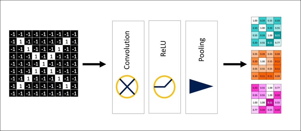
Figure 27: Basic Unit of CNN showing a combination of Convolution, ReLu, and Pooling.
Thus, these layers can be combined or "deep-stacked", as shown in the following figure, to form a complex network that gives a small pool of images as output:

Figure 28: Deep-stacking the basic units repeatedly to form CNN layers.
The output layer is a fully connected network as shown, which uses a voting technique and learns the weights for the desired output. The fully connected output layer can be stacked too.

Figure 29: Fully connected layer as output of CNN.
Thus, the final CNNs can be completely illustrated as follows:
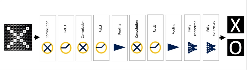
Figure 30: CNNS with all layers showing inputs and outputs.
As before, gradient descent is selected as the learning technique using the loss functions to compute the difference and propagate the error backwards.
CNN's can be used in other domains such as voice pattern recognition, text mining, and so on, if the mapping of the data to the "image" can be successfully done and "local spatial" patterns exist. The following figure shows one of the ways of mapping sound and text to images for CNN usage:

Figure 31: Illustration of mapping between temporal data, such as voice to spatial data, to an image.
Normal deep networks are used when you have finite inputs and there is no interdependence between the input examples or instances. When there are variable length inputs and there are temporal dependencies between them, that is, sequence related data, neural networks must be modified to handle such data. Recurrent Neural Networks (RNN) are examples of neural networks that are used widely to solve such problems, and we will discuss them in the following sections. RNNs are used in many sequence-related problems such as text mining, language modeling, bioinformatics data modeling, and so on, to name a few areas that fit this meta-level description (References [18 and 21]).
We will describe the simplest unit of the RNN first and then shown how it is combined to understand it functionally and mathematically and illustrate how different components interact and work.

Figure 32: Difference between an artificial neuron and a neuron with feedback.
Let's consider the basic input, a neuron with activation, and its output at a given time t:


A neuron with feedback keeps a matrix WR to incorporate previous output at time t-1 and the equations are:


Figure 33: Chain of neurons with feedbacks connected together.
The basic RNN stacks the structure of hidden units as shown with feedback connected from the previous layer. At activation at time t, it depends not only on x(t) as input, but also on the previous unit given by WRh(t-1). The weights in the feedback connection of RNN are generally the same across all the units, WR. Also, instead of emitting output at the very end of the feed-forward neural network, each unit continuously emits an output that can be used in the loss function calculation.
Working with RNNs presents some challenges that are specific to them but there are common problems that are also encountered in other types of neural net.
- The gradient used from the output loss function at any time t of the unit has dependency going back to the first unit or t=0, as shown in the following figure. This is because the partial derivative at the unit is dependent on the previous unit, since:
Backpropagation through time (BPTT) is the term used to illustrate the process.

Figure 34: Backpropagation through time.
- Similar to what we saw in the section on feed-forward neural networks, the cases of exploding and vanishing gradient become more pronounced in RNNs due to the connectivity of units as discussed previously.
- Some of the solutions for exploding gradients are:
- Truncated BPTT is a small change to the BPTT process. Instead of propagating the learning back to time t=0, it is truncated to a fixed time backward to t=k.
- Gradient Clipping to cut the gradient above a threshold when it shoots up.
- Adaptive Learning Rate. The learning rate adjusts itself based on the feedback and values.
- Some of the solutions for vanishing gradients are:
- Using ReLU as the activation function; hence the gradient will be 1.
- Adaptive Learning Rate. The learning rate adjusts itself based on the feedback and values.
- Using extensions such as Long Short Term Memory (LSTM) and Gated Recurrent Units (GRUs), which we will describe next.
There are many applications of RNNs, for example, in next letter predictions, next word predictions, language translation, and so on.

Figure 35: Showing some applications in next letter/word predictions using RNN structures.
One of the neural network architectures or modifications to RNNs that addresses the issue of vanishing gradient is known as long short term memory or LSTM. We will explain some building blocks of LSTM and then put it together for our readers.
The first modification to RNN is to change the feedback learning matrix to 1, that is, WR = 1, as shown in the following figure:

Figure 36: Building blocks of LSTM where the feedback matrix is set to 1.
This will ensure the inputs from older cell or memory units are passed as-is to the next unit. Hence some modifications are needed.
The output gate, as shown in the following figure, combines two computations. The first is the output from the individual unit, passed through an activation function, and the second is the output of the older unit that has been passed through a sigmoid using scaling.

Figure 37: Building block Output Gate for LSTM.
Mathematically, the output gate at the unit is given by:


The forget gate is between the two memory units. It generates 0 or 1 based on learned weights and transformations. The forget gate is shown in the following figure:
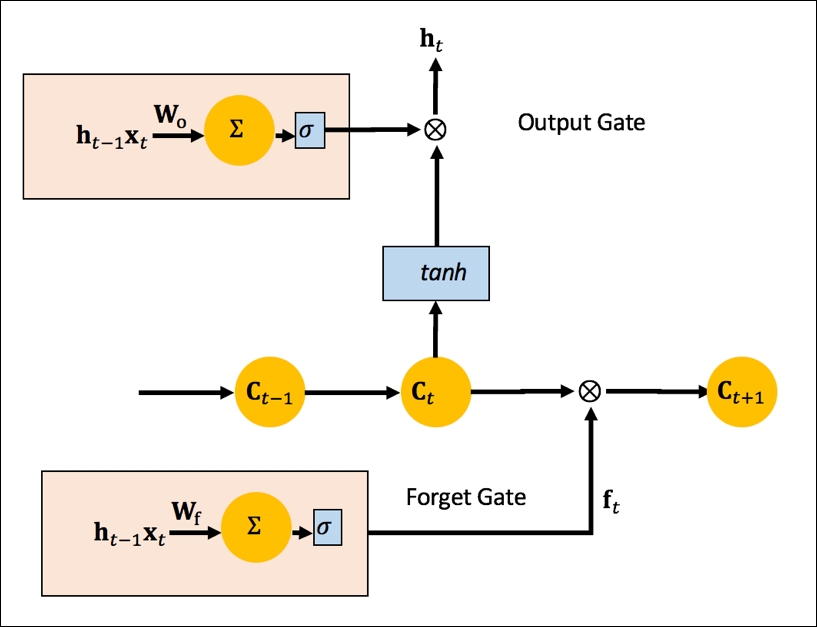
Figure 38: Building block Forget Gate addition to LSTM.
Mathematically, ![]() can be seen as the representation of the forget gate. Next, the input gate and the new gate are combined, as shown in the following figure:
can be seen as the representation of the forget gate. Next, the input gate and the new gate are combined, as shown in the following figure:

Figure 39: Building blocks New Gate and Input Gate added to complete LSTM.
The new memory generation unit uses the current input xt and the old state ht-1 through an activation function and generates a new memory Ct. The input gate combines the input and the old state and determines whether the new memory or the input should be preserved.
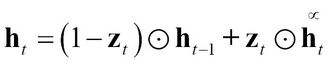
Thus, the update equation looks like this: