 Matrix
by Krishna Choppella, Dr. Uday Kamath, Boštjan Kaluža, Jennifer L. Reese, Richard M
Machine Learning: End-to-End guide for Java developers
Matrix
by Krishna Choppella, Dr. Uday Kamath, Boštjan Kaluža, Jennifer L. Reese, Richard M
Machine Learning: End-to-End guide for Java developers
- Machine Learning: End-to-End guide for Java developers
- Table of Contents
- Machine Learning: End-to-End guide for Java developers
- Credits
- Preface
- 1. Module 1
- 1. Getting Started with Data Science
- Problems solved using data science
- Understanding the data science problem - solving approach
- Acquiring data for an application
- The importance and process of cleaning data
- Visualizing data to enhance understanding
- The use of statistical methods in data science
- Machine learning applied to data science
- Using neural networks in data science
- Deep learning approaches
- Performing text analysis
- Visual and audio analysis
- Improving application performance using parallel techniques
- Assembling the pieces
- Summary
- 2. Data Acquisition
- 3. Data Cleaning
- 4. Data Visualization
- 5. Statistical Data Analysis Techniques
- 6. Machine Learning
- 7. Neural Networks
- 8. Deep Learning
- 9. Text Analysis
- 10. Visual and Audio Analysis
- 11. Mathematical and Parallel Techniques for Data Analysis
- 12. Bringing It All Together
- 1. Getting Started with Data Science
- 2. Module 2
- 1. Applied Machine Learning Quick Start
- 2. Java Libraries and Platforms for Machine Learning
- 3. Basic Algorithms – Classification, Regression, and Clustering
- 4. Customer Relationship Prediction with Ensembles
- 5. Affinity Analysis
- 6. Recommendation Engine with Apache Mahout
- 7. Fraud and Anomaly Detection
- 8. Image Recognition with Deeplearning4j
- 9. Activity Recognition with Mobile Phone Sensors
- 10. Text Mining with Mallet – Topic Modeling and Spam Detection
- 11. What is Next?
- A. References
- 3. Module 3
- 1. Machine Learning Review
- Machine learning – history and definition
- What is not machine learning?
- Machine learning – concepts and terminology
- Machine learning – types and subtypes
- Datasets used in machine learning
- Machine learning applications
- Practical issues in machine learning
- Machine learning – roles and process
- Machine learning – tools and datasets
- Summary
- 2. Practical Approach to Real-World Supervised Learning
- Formal description and notation
- Data transformation and preprocessing
- Feature relevance analysis and dimensionality reduction
- Model building
- Model assessment, evaluation, and comparisons
- Case Study – Horse Colic Classification
- Summary
- References
- 3. Unsupervised Machine Learning Techniques
- Issues in common with supervised learning
- Issues specific to unsupervised learning
- Feature analysis and dimensionality reduction
- Clustering
- Outlier or anomaly detection
- Real-world case study
- Summary
- References
- 4. Semi-Supervised and Active Learning
- Semi-supervised learning
- Active learning
- Case study in active learning
- Summary
- References
- 5. Real-Time Stream Machine Learning
- Assumptions and mathematical notations
- Basic stream processing and computational techniques
- Concept drift and drift detection
- Incremental supervised learning
- Incremental unsupervised learning using clustering
- Modeling techniques
- Partition based
- Hierarchical based and micro clustering
- Density based
- Grid based
- Validation and evaluation techniques
- Key issues in stream cluster evaluation
- Evaluation measures
- Cluster Mapping Measures (CMM)
- V-Measure
- Other external measures
- Unsupervised learning using outlier detection
- Case study in stream learning
- Summary
- References
- 6. Probabilistic Graph Modeling
- Probability revisited
- Graph concepts
- Bayesian networks
- Representation
- Inference
- Learning
- Learning parameters
- Learning structures
- Measures to evaluate structures
- Methods for learning structures
- Constraint-based techniques
- Search and score-based techniques
- 7. Deep Learning
- Multi-layer feed-forward neural network
- Inputs, neurons, activation function, and mathematical notation
- Multi-layered neural network
- Structure and mathematical notations
- Activation functions in NN
- Training neural network
- Empirical risk minimization
- Parameter initialization
- Loss function
- Gradients
- Feed forward and backpropagation
- How does it work?
- Regularization
- L2 regularization
- L1 regularization
- Limitations of neural networks
- Deep learning
- Building blocks for deep learning
- Rectified linear activation function
- Restricted Boltzmann Machines
- Autoencoders
- Unsupervised pre-training and supervised fine-tuning
- Deep feed-forward NN
- Deep Autoencoders
- Deep Belief Networks
- Deep learning with dropouts
- Sparse coding
- Convolutional Neural Network
- CNN Layers
- Recurrent Neural Networks
- Building blocks for deep learning
- Case study
- Summary
- References
- 8. Text Mining and Natural Language Processing
- NLP, subfields, and tasks
- Text categorization
- Part-of-speech tagging (POS tagging)
- Text clustering
- Information extraction and named entity recognition
- Sentiment analysis and opinion mining
- Coreference resolution
- Word sense disambiguation
- Machine translation
- Semantic reasoning and inferencing
- Text summarization
- Automating question and answers
- Issues with mining unstructured data
- Text processing components and transformations
- Topics in text mining
- Tools and usage
- Summary
- References
- NLP, subfields, and tasks
- 9. Big Data Machine Learning – The Final Frontier
- What are the characteristics of Big Data?
- Big Data Machine Learning
- Batch Big Data Machine Learning
- Case study
- Business problem
- Machine Learning mapping
- Data collection
- Data sampling and transformation
- Spark MLlib as Big Data Machine Learning platform
- A. Linear Algebra
- B. Probability
- D. Bibliography
- Index
- Empirical risk minimization
- Multi-layer feed-forward neural network
- Modeling techniques
- 1. Machine Learning Review
A matrix is a two-dimensional array of numbers. Each element can be indexed by its row and column position. Thus, a 3 x 2 matrix:

Swapping columns for rows in a matrix produces the transpose. Thus, the transpose of A is a 2 x 3 matrix:

Matrix addition is defined as element-wise summation of two matrices with the same shape. Let A and B be two m x n matrices. Their sum C can be written as follows:
Ci,j = Ai,j + Bi,j
Multiplication with a scalar produces a matrix where each element is scaled by the scalar value. Here A is multiplied by the scalar value d:
Two matrices A and B can be multiplied if the number of columns of A equals the number of rows of B. If A has dimensions m x n and B has dimensions n x p, then the product AB has dimensions m x p:

Distributivity over addition: A(B + C) = AB + AC
Associativity: A(BC) = (AB)C
Non-commutativity: AB ≠ BA
Vector dot-product is commutative: xTy = yTx
Transpose of product is product of transposes: (AB)T = ATBT
There is a special importance to the product of a matrix and a vector in linear algebra. Consider the product of a 3 x 2 matrix A and a 2 x 1 vector x producing a 3 x 1 vector y:


(C)
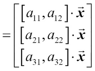
(R)
It is useful to consider two views of the preceding matrix-vector product, namely, the column picture (C) and the row picture (R). In the column picture, the product can be seen as a linear combination of the column vectors of the matrix, whereas the row picture can be thought of as the dot products of the rows of the matrix with the vector ![]()
The product of a matrix with its inverse is the Identity matrix. Thus:

The matrix inverse, if it exists, can be used to solve a system of simultaneous equations represented by the preceding vector-matrix product equation. Consider a system of equations:
x1 + 2x2 = 3
3x1 + 9x2 = 21
This can be expressed as an equation involving the matrix-vector product:

We can solve for the variables x1 and x2 by multiplying both sides by the matrix inverse:


The matrix inverse can be calculated by different methods. The reader is advised to view Prof. Strang's MIT lecture: bit.ly/10vmKcL.
Matrices can be decomposed to factors that can give us valuable insight into the transformation that the matrix represents. Eigenvalues and eigenvectors are obtained as the result of eigendecomposition. For a given square matrix A, an eigenvector is a non-zero vector that is transformed into a scaled version of itself when multiplied by the matrix. The scalar multiplier is the eigenvalue. All scalar multiples of an eigenvector are also eigenvectors:
A v = λ v
In the preceding example, v is an eigenvector and λ is the eigenvalue.
The eigenvalue equation of matrix A is given by:
(A — λ I)v = 0
The non-zero solution for the eigenvalues is given by the roots of the characteristic polynomial equation of degree n represented by the determinant:

The eigenvectors can then be found by solving for v in Av = λ v.
Some matrices, called diagonalizable matrices, can be built entirely from their eigenvectors and eigenvalues. If Λ is the diagonal matrix with the eigenvalues of matrix A on its principal diagonal, and Q is the matrix whose columns are the eigenvectors of A:

Then A = Q Λ Q-1.
SVD is a decomposition of any rectangular matrix A of dimensions n x p and is written as the product of three matrices:

U is defined to be n x n, S is a diagonal n x p matrix, and V is p x p. U and V are orthogonal matrices; that is:

The diagonal values of S are called the singular values of A. Columns of U are called left singular vectors of A and those of V are called right singular vectors of A. The left singular vectors are orthonormal eigenvectors of ATA and the right singular vectors are orthonormal eigenvectors of AAT.
The SVD representation expands the original data into a coordinate system such that the covariance matrix is a diagonal matrix.
-
No Comment