
As we saw in the first section, the area of text mining and performing Machine Learning on text spans a wide range of topics. Each topic discussed has some customizations to the mainstream algorithms, or there are specific algorithms that have been developed to perform the task called for in that area. We have chosen four broad topics, namely, text categorization, topic modeling, text clustering, and named entity recognition, and will discuss each in some detail.
The text classification problem manifests itself in different applications, such as document filtering and organization, information retrieval, opinion and sentiment mining, e-mail spam filtering, and so on. Similar to the classification problem discussed in Chapter 2, Practical Approach to Real-World Supervised Learning, the general idea is to train on the training data with labels and to predict the labels of unseen documents.
As discussed in the previous section, the preprocessing steps help to transform the unstructured document collection into well-known numeric or categorical/binary structured data arranged in terms of a document-term matrix. The choice of performing some preprocessing steps, such as stemming or customizing stop words, depends on the data and applications. The feature choice is generally basic lexical features, n-grams of words as terms, and only in certain cases do we use the entire text as a string without breaking it into terms or tokens. It is common to use binary feature representation or frequency-based representation for document-term structured data. Once this transformation is complete, we do feature selection using univariate analysis, such as information gain or chi-square, to choose discriminating features above certain thresholds of scores. One may also perform feature transformation and dimensionality reduction such as PCA or LSA in many applications.
There is a wide range in the choice of classifiers once we get structured data from the preceding process. In the research as well as in commercial applications, we see the use of most of the common modeling techniques, including linear (linear regression, logistic regression, and so on), non-linear (SVM, neural networks, KNN), generative (naïve bayes, bayesian networks), interpretable (decision trees, rules), and ensemble-based (bagging, boosting, random forest) classifiers. Many algorithms use similarity or distance metrics, of which cosine distance is the most popular choice. In certain classifiers, such as SVM, the string representation of the document can be used as is, with the right choice of string kernels and similarity-based metrics on strings to compute the dot products.
Validation and evaluation methods are similar to supervised classification methodologies—splitting the data into train/validation/test, training on training data, tuning parameters of algorithm(s) on validation data, and estimating the performance of the models on hold-out or test data.
Since most of text classification involves a large number of documents, and the target classes are rare, the metrics used for evaluation, tuning, or choosing algorithms are in most cases precision, recall, and F-score measure, as follows:


A topic is a distribution over a fixed vocabulary. Topic modeling can be defined as an ability to capture different core ideas or themes in various documents. This has a wide range of applications, such as the summarization of documents, understanding reasons for sentiments, trends, the news, and many others. The following figure shows how topic modeling can discern a user-specified number k of topics from a corpus and then, for every document, assign proportions representing how much of each topic is found in the document:

Figure 13: Probabilistic topic weights assignment for documents
There are quite a few techniques for performing topic modeling using supervised and unsupervised learning in the literature (References [13]). We will discuss the most common technique known as probabilistic latent semantic index (PLSI).
The idea of PLSA, as in the LSA for feature reduction, is to find latent concepts hidden in the corpus by discovering the association between co-occurring terms and treating the documents as mixtures of these concepts. This is an unsupervised technique, similar to dimensionality reduction, but the idea is to use it to model the mixture of topics or latent concepts in the document (References [12]).
As shown in the following figure, the model may associate terms occurring together often in the corpus with a latent concept, and each document can then be said to exhibit that topic to a smaller or larger extent:

Figure 14: Latent concept of Baseball capturing the association between documents and related terms
The inputs are:

The output is:
- k topics identified T = {T1, T2,…Tk}.
- For each document, coverage of the topic given in the document di can be written as = {pi1, pi2, …pik}, where pijis the probability of the document di covering the topic Tj.
Implementations of PLSA generally follow the steps described here:
- Basic preprocessing steps as discussed previously, such as tokenization, stop words removal, stemming, dictionary of words formation, feature extraction (unigrams or n-grams, and so on), and feature selection (unsupervised techniques) are carried out, if necessary.
- The problem can be reduced to estimating the distribution of terms in a document, and, given the distribution, choosing the topic based on the maximum terms corresponding to the topic.
- Introducing a "latent variable" z helps us to select whether the term belongs to a topic. Note that z is not "observed", but we assume that it is related to picking the term from the topic. Thus, the probability of the term t given the document t can be expressed in terms of this latent variable as:
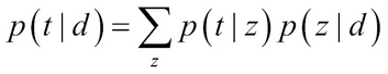
- By using two sets of variables (?, p) the equation can be written as:

Here, p(t|z; ?) is the probability of latent concepts in terms and p(z|d; p) is the probability of latent concepts in document-specific mixtures.
- Using log-likelihood to estimate the parameters to maximize:

- Since this equation involves nonconvex optimization, the EM algorithm is often used to find the parameters iteratively until convergence is reached or the total number of iterations are completed (References [6]):
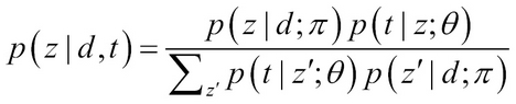
- The E-step of the EM algorithm is used to determine the posterior probability of the latent concepts. The probability of term t occurring in the document d, can be explained by the latent concept z as:
- The M-step of the EM algorithm uses the values obtained from the E-step, that is, p(z|d, t) and does parameter estimation as:

 = how often the term t is associated with concept z:

 = how often document d is associated with concept z.
- The E-step of the EM algorithm is used to determine the posterior probability of the latent concepts. The probability of term t occurring in the document d, can be explained by the latent concept z as:
The advantages and limitations are as follows:
- Though widely used, PLSA has some drawbacks that have been overcome by more recent techniques.
- The unsupervised nature of the algorithm and its general applicability allows it to be used in a wide variety of similar text mining applications, such as clustering documents, associating topics related to authors/time, and so on.
- PLSA with EM algorithms, as discussed in previous chapters, face the problem of getting "stuck in local optima", unlike other global algorithms, such as evolutionary algorithms.
- PLSA algorithms can only do topic identification in known documents, but cannot do any predictive modeling. PLSA has been generalized and is known as latent dirichlet allocation (LDA) to overcome this (References [14]).
The goal of clustering, as seen in Chapter 3, Unsupervised Machine Learning Techniques, is to find groups of data, text, or documents that are similar to one another within the group. The granularity of unstructured data can vary from small phrases or sentences, paragraphs, and passages of text to a collection of documents. Text clustering finds its application in many domains, such as information retrieval, summarization, topic modeling, and document classification in unsupervised situations, to name a few. Traditional techniques in clustering can be employed once the unstructured text data is transformed into structured data via preprocessing. The difficulty with traditional clustering techniques is the high-dimensional and sparse nature of the dataset obtained using the transformed document-term matrix representation. Many traditional clustering algorithms work only on numeric values of features. Because of this constraint, categorical or binary representation of terms cannot be used and often TF or TF-IDF are used for representation of the document-term matrix.
In this section, we will discuss some of the basic processes and techniques in clustering. We will start with pre-processing and transformations and then discuss some techniques that are widely used and the modifications made to them.
Most of the pre-processing steps discussed in this section are normally used to get either unigram or n-gram representation of terms in documents. Dimensionality reduction techniques, such as LSA, are often employed to transform the features into smaller latent space.
The techniques for clustering in text include probabilistic models, as well as those that use distance-based methods, which are familiar to us from when we learned about structured data. We will also discuss Non-negative Matrix Factorization (NNMF) as an effective technique with good performance and interpretability.
There is commonality between topic modeling and text clustering in generative methods. As shown in the following figure, clustering associates a document with a single cluster (generally), compared to topic modeling where each document can have a probability of coverage in multiple topics. Every word in topic modeling can be generated by multiple topics in an independent manner, whereas in clustering all the words are generated from the same cluster:

Figure 15: Exclusive mapping of documents to K-Clusters
Mathematically, this can be explained using two topics T = {T1, T2} and two clusters c = {c1, c2}.
In clustering, the likelihood of the document can be given as:

If the document has, say, L terms, this can be further expanded as:

Thus, once you "assume" a cluster, all the words come from that cluster. The product of all terms is computed, followed by the summation across all clusters.
In topic modeling, the likelihood of the document can be given as:

Thus, each term ti can be picked independently from topics and hence summation is done inside and the product is done outside.
The inputs are:
The output is:
- k clusters identified c = {c1, c2, … ck}.
- For each document, p(di) is mapped to one of the clusters k.
Here are the steps:
-
Basic preprocessing steps as discussed previously, such as tokenization, stop words removal, stemming, dictionary of words formation, feature extraction (unigrams or n-grams, and so on) of terms, feature transformations (LSA), and even feature selection. Let t be the terms in the final feature set; they correspond to the dictionary or vocabulary
 .
.
- Similar to PLSA, we introduce a "latent variable", z, which helps us to select whether the document belonging to the cluster falls in the range of z ={1, 2, … k} corresponding to the clusters. Let the ? parameter be the parameter we estimate for each latent variable such that p(?i) corresponds to the probability of cluster z = i.
- The probability of a document belonging to a cluster is given by p(?i), and every term in the document generated from that cluster is given by p(t|?i). The likelihood equation can be written as:

Note that instead of going through the documents, it is rewritten with terms t in the vocabulary
raised to the number of times that term appears in the document. - Perform the EM algorithm in a similar way to the method we used previously to estimate the parameters as follows:
- The E-step of the EM algorithm is used to infer the cluster from which the document was generated:

- The M-step of the EM algorithm is used to re-estimate the parameters using the result of the E-step, as shown here:


- The E-step of the EM algorithm is used to infer the cluster from which the document was generated:
-
The final probability estimate for each document can be done using either the maximum likelihood or by using a Bayesian algorithm with prior probabilities, as shown here:
 or
or 
- Generative-based models have similar advantages to LSA and PLSA, where we get a probabilistic score for documents in clusters. By applying domain knowledge or priors using cluster size, the assignments can be further fine-tuned.
- The disadvantages of the EM algorithm having to do with getting stuck in local optima and being sensitive to the starting point are still true here.
Most distance-based clustering algorithms rely on the similarity or the distance measure used to determine how far apart instances are from each other in feature space. Normally in datasets with numeric values, Euclidean distance or its variations work very well. In text mining, even after converting unstructured text to structured features of terms with numeric values, it has been found that the cosine and Jaccard similarity functions perform better.
Often, Agglomerative or Hierarchical clustering, discussed in Chapter 3, Unsupervised Machine Learning Techniques, are used, which can merge documents based on similarity, as discussed previously. Merging the documents or groups is often done using single linkage, group average linkage, and complete linkage techniques. Agglomerative clustering also results in a structure that can be used for information retrieval and the searching of documents.
The partition-based clustering techniques k-means and k-medoids accompanied by h a suitable similarity or distance method are also employed. The issue with k-means, as indicated in the discussion on clustering techniques, is the sensitivity to starting conditions along with computation space and time. k-medoids are sensitive to the sparse data structure and also have computation space and time constraints.
Non-negative matrix factorization is another technique used to factorize a large data-feature matrix into two non-negative matrices, which not only perform the dimensionality reduction, but are also easier to inspect. NMF has gained popularity for document clustering, and many variants of NMF with different optimization functions have now been shown to be very effective in clustering text (References [15]).
The inputs are:
The output is:
- k clusters identified c = {c1, c2, … ck} with documents assigned to the clusters.
The mathematical details and interpretation of NMF are given in the following:
- The basic idea behind NMF is to factorize the input matrix using low-rank approximation, as follows:

- A non-linear optimization function is used as:

This is convex in W or H, but not in both, resulting in no guarantees of a global minimum. Various algorithms that use constrained least squares, such as mean-square error and gradient descent, are used to solve the optimization function.
- The interpretation of NMF, especially in understanding the latent topics based on terms, makes it very useful. The input Am x n of terms and documents, can be represented in low rank approximation as Wm x k Hk x n matrices, where Wm x k is the term-topic representation whose columns are NMF basis vectors. The non zero elements of column 1 of W, given by W1, correspond to particular terms. Thus, the wij can be interpreted as a basis vector Wi about the terms j. The Hi1 can be interpreted as how much the document given by doc 1 has affinity towards the direction of the topic vector Wi.
- From the paper (References [18]) it was clearly shown how the basis vectors obtained for the medical abstracts, known as the Medlars dataset, creates highly interpretable basis vectors. The highest weighted terms in these basis vectors directly correspond to the concept, for example, W1 corresponds to the topic related to "heart" and W5 is related to "developmental disability".

Figure 16: From Langville et al (2006) showing some basis vectors for medical datasets for interpretability.
NMF has been shown to be almost equal in performance with top algorithms, such as LSI, for information retrieval and queries:
- Scalability, computation, and storage is better in NMF than in LSA or LSI using SVD.
- NMF has a problem with optimization not being global and getting stuck in local minima.
- NMF generation of factors depends on the algorithms for optimization and the parameters chosen, and is not unique.
In the case of labeled datasets, all the external measures discussed in Chapter 3, Unsupervised Machine Learning Techniques, such as F-measure and Rand Index are useful in evaluating the clustering techniques. When the dataset doesn't have labels, some of the techniques described as the internal measures, such as the Davies–Bouldin Index, R-Squared, and Silhouette Index, can be used.
The general good practice is to adapt and make sure similarity between the documents, as discussed in this section, is used for measuring closeness, remoteness, and spread of the cluster when applied to text mining data. Similarly usage depends on the algorithm and some relevance to the problem too. In distance-based partition algorithms, the similarity of the document can be computed with the mean vector or the centroid. In hierarchical algorithms, similarity can be computed with most similar or dissimilar documents in the group.
Named entity recognition (NER) is one of the most important topics in information retrieval for text mining. Many complex mining tasks, such as the identification of relations, annotations of events, and correlation between entities, use NER as the initial component or basic preprocessing step.
Historically, manual rules-based and regular expression-based techniques were used for entity recognition. These manual rules relied on basic pre processing, using POS tags as features, along with hand-engineered features, such as the presence of capital words, usage of punctuations prior to words, and so on.
Statistical learning-based techniques are now used more for NER and its variants. NER can be mapped to sequence labeling and prediction problems in Machine Learning. BIO notation, where each entity type T has two labels B-T and I-T corresponding to beginning and intermediate, respectively, is labeled, and learning involves finding the pattern and predicting it in unseen data. The O represents an outside or unrelated entity in the sequence of text. The entity type T is further classified into Person, Organization, Data, and location in the most basic form.
In this section, we will discuss the two most common algorithms used: generative-based hidden Markov models and discriminative-based maximum entropy models.
Though we are discussing these algorithms in the context of Named Entity Recognition, the same algorithms and processes can be used for other NLP tasks such as POS Tagging, where tags are associated with a sequence rather than associating the NER classes.
Hidden Markov models, as explained in Chapter 6, Probabilistic Graph Modeling, are the sequence-based generative models that assume an underlying distribution that generates the sequences. The training data obtained by labeling sequences with the right NER classes can be used to learn the distribution and parameters, so that for unseen future sequences, effective predictions can be performed.
The training data consists of text sequences x ={x1, x2, ... xn} where each xi is a word in the text sequence and labels for each word are available as y ={y1, y2, ... yn}. The algorithm generates a model so that on testing on unseen data, the labels for new sequences can be generated.
- In the simplest form, a Markov assumption is made, which is that the hidden states and labels of the sequences are only dependent on the previous state. An adaptation to the sequence of words with labels is shown in the following figure:

Figure 17: Text sequence and labels corresponding to NER in Hidden Markov Chain
- The HMM formulation of the sequence classification helps in estimating the joint probability maximized on training data:

- Each yi is assumed to be generated based on yi–1 and xi. The first word in the entity is generated conditioned on current and previous labels, that is, yi and yi–1. If the instance is already a Named entity, then conditioning is only on previous instances, that is, xi–1. Outside words such as "visited" and "in" are considered "not a name class".
- The HMM formulation with the forward-backward algorithm can be used to determine the likelihood of a sequence of observations with parameters learned from the training data.
The advantages and limitations are as follows:
Maximum entropy Markov model (MEMM) is a popular NER technique that uses the concept of Markov chains and maximum entropy models to learn and predict the named entities (References [16] and [17]).
The training data consists of text sequences x ={x1, x2, ... xn} where each xi is a word in the text sequence and labels for each word are available as y ={y1, y2, ... yn}. The algorithm generates models so that, on testing on unseen data, the labels for new sequences can be generated.
The following illustrates how the MEMM method is used for learning named entities.
- The features in MEMM can be word features or other types of features, such as "isWordCapitalized", and so on, which gives it a bit more context and improves performance compared to HMM, where it is only word-based.
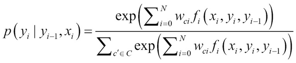
- Next, let us look at a maximum entropy model known as a MaxEnt model, which is an exponential probabilistic model, but which can also be seen as a multinomial logistic regression model. In basic MaxEnt models, given the features {f1, f2 … fN} and classes c1, c2 … cC, weights for these features are learned {wc1, wc2 … wcN} per class using optimization methods from the training data, and the probability of a particular class can be estimated as:

- The feature fi is formally written as fi(c, x), which means the feature fi for class c and observation x. The fi(c, x) is generally binary with values 1/0 in most NER models. Thus, it can be written as:

Maximum likelihood based on the probability of prediction across class can be used to select a single class:

- For every word, we use the current word, the features from "nearby" words, and the predictions on the nearby words to create a joint probability model. This is also called local learning as the chunks of test and distribution are learned around local features corresponding to the word.
Mathematically, we see how a discriminative model is created from current word and last prediction as:


Generalizing for the k features:

- Thus, in MEMM we compute the probability of the state, which is the class in NER, and even though we condition on prediction of nearby words given by yi–1, in general we can use more features, and that is the advantage over the HMM model discussed previously:


Figure 18 : Text Sequences and observation probabilities with labels
- The Viterbi algorithm is used to perform the estimation of class for the word or decoding/inferencing in HMM, that is, to get estimates for p(yi|yi–1, Xi)
- Finally, the MaxEnt model is used to estimate the weights as before using the optimization methods for state changes in general:
In the last few years, Deep Learning and its application to various areas of NLP has shown huge success and is considered the cutting edge of technology these days. The main advantage of using Deep Learning lies in a small subset of tools and methods, which are useful in a wide variety of NLP problems. It solves the basic issue of feature engineering and carefully created manual representations by automatically learning them, and thus solves the issue of having a large number of language experts dealing with a wide range of problems, such as text classification, sentiment analysis, POS tagging, and machine translation, to name a few. In this section, we will try to cover important concepts and research in the area of Deep Learning and NLP.
In his seminal paper, Bengio introduced one of the most important building blocks for deep learning known as word embedding or word vector (References [20]). Word embedding can be defined as a parameterized function that maps words to a high dimensional vector (usually 25 to 500 dimensions based on the application).
Formally, this can be written as ![]() .
.
For example, ![]() and
and ![]() , and so on.
, and so on.
A neural network (R) whose inputs are the words from sentences or n-grams of sentences with binary classification, such as whether the sequence of words in n-grams are valid or not, is used to train and learn the W and R:

Figure 19: A modular neural network learning 5-gram words for valid–invalid classification
For example:
- R(W(cat),W(sat ),W(on),W(the),W(mat)) = 1(valid)
- R(W(cat),W(sat),W(on),W(the),W(mat)) = 0 (Invalid)
The idea of training these sentences or n-grams is not only to learn the correct structure of the phrases, but also the right parameters for W and R. The word embeddings can also be projected on to a lower dimensional space, such as a 2D space, using various linear and non linear feature reduction/visualization techniques introduced in Chapter 3, Unsupervised Machine Learning Techniques, which humans can easily visualize. This visualization of word embeddings in two dimensions using techniques such as t-SNE discovers important information about the closeness of words based on semantic meaning and even clustering of words in the area, as shown in the following figure:

Figure 20: t-SNE representation of a small section of the entire word mappings. Numbers in Roman numerals and words are shown clustered together on the left, while semantically close words are clustered together on the right.
Further extending the concepts, both Collobert and Mikolov showed that the side effects of learning the word embeddings can be very useful in a variety of NLP tasks, such as similar phrase learning (for example, W("the color is red")) ? W("the color is yellow")), finding synonyms (for example, W("nailed")) ? W("smashed")), analogy mapping (for example, W("man")?W("woman") then W("king")?W("queen")), and even complex relationship mapping (for example, W("Paris")?W("France") then W("Tokyo")?W("Japan")) (References [21 and 22]).
The extension of word embedding concepts towards a generalized representation that helps us reuse the representation with various NLP problems (with minor extensions) has been the main reason for many recent successes of Deep Learning in NLP. Socher, in his research, extended the word embeddings concept to produce bilingual word embeddings, that is, embed words from two different languages, such as Chinese (Mandarin) and English into a shared space (References [23]). By learning two language word embeddings independently of each other and then projecting them in a same space, his work gives us interesting insights into word similarities across languages that can be extended for Machine Translation. Socher also did interesting work on projecting the images learned from CNNs with the word embedding in to the same space for associating words with images as a basic classification problem (References [24]). Google, around the same time, has also been working on similar concepts, but at a larger scale for word-image matching and learning (References [26]).
Extending the word embedding concept to have combiners or association modules that can help combine the words, words-phrases, phrases-phrases in all combinations to learn complex sentences has been the idea of Recursive Neural Networks. The following figure shows how complex association ((the cat)(sat(on (the mat)))) can be learned using Recursive Neural Networks. It also removes the constraint of a "fixed" number of inputs in neural networks because of the ability to recursively combine:

Figure 21: Recursive Neural Network showing how complex phrases can be learned.
Recursive Neural Networks have been showing great promise in NLP tasks, such as sentiment analysis, where association of one negative word at the start of many positive words has an overall negative impact on sentences, as shown in the following figure:

Figure 22: A complex sentence showing words with negative (as red circle), positive (green circle), and neutral (empty with 0) connected through RNN with overall negative sentiment.
The concept of recursive neural networks is now extended using the building blocks of encoders and decoders to learn reversible sentence representation—that is, reconstructing the original sentence with roughly the same meaning from the input sentence (References [27]). This has become the central core theme behind Neural Machine Translation. Modeling conversations using the encoder-decoder framework of RNNs has also made huge breakthroughs (References [28]).