
Supervised learning is the key concept behind amazing things such as voice recognition, e-mail spam filtering, face recognition in photos, and detecting credit card frauds. More formally, given a set D of learning examples described with features, X, the goal of supervised learning is to find a function that predicts a target variable, Y. The function f that describes the relation between features X and class Y is called a model:
The general structure of supervised learning algorithms is defined by the following decisions (Hand et al., 2001):
- Define the task.
- Decide on the machine learning algorithm, which introduces specific inductive bias, that is, apriori assumptions that it makes regarding the target concept.
- Decide on the score or cost function, for instance, information gain, root mean square error, and so on.
- Decide on the optimization/search method to optimize the score function.
- Find a function that describes the relation between X and Y.
Many decisions are already made for us by the type of the task and dataset that we have. In the following sections, we will take a closer look at the classification and regression methods and the corresponding score functions.
Classification can be applied when we deal with a discrete class, and the goal is to predict one of the mutually-exclusive values in the target variable. An example would be credit scoring, where the final prediction is whether the person is credit liable or not. The most popular algorithms include decision tree, naïve Bayes classifier, support vector machines, neural networks, and ensemble methods.
Decision tree learning builds a classification tree, where each node corresponds to one of the attributes, edges correspond to a possible value (or intervals) of the attribute from which the node originates, and each leaf corresponds to a class label. A decision tree can be used to visually and explicitly represent the prediction model, which makes it a very transparent (white box) classifier. Notable algorithms are ID3 and C4.5, although many alternative implementations and improvements (for example, J48 in Weka) exist.
Given a set of attribute values, a probabilistic classifier is able to predict a distribution over a set of classes, rather than an exact class. This can be used as a degree of certainty, that is, how sure the classifier is in its prediction. The most basic classifier is naïve Bayes, which happens to be the optimal classifier if, and only if, the attributes are conditionally independent. Unfortunately, this is extremely rare in practice.
There is really an enormous subfield denoted as probabilistic graphical models, comprising of hundreds of algorithms; for example, Bayesian network, dynamic Bayesian networks, hidden Markov models, and conditional random fields that can handle not only specific relationships between attributes, but also temporal dependencies. Karkera (2014) wrote an excellent introductory book on this topic, Building Probabilistic Graphical Models with Python, while Koller and Friedman (2009) published a comprehensive theory bible, Probabilistic Graphical Models.
Any linear model can be turned into a non-linear model by applying the kernel trick to the model—replacing its features (predictors) by a kernel function. In other words, the kernel implicitly transforms our dataset into higher dimensions. The kernel trick leverages the fact that it is often easier to separate the instances in more dimensions. Algorithms capable of operating with kernels include the kernel perceptron, Support Vector Machines (SVM), Gaussian processes, PCA, canonical correlation analysis, ridge regression, spectral clustering, linear adaptive filters, and many others.
Artificial neural networks are inspired by the structure of biological neural networks and are capable of machine learning, as well as pattern recognition. They are commonly used for both regression and classification problems, comprising a wide variety of algorithms and variations for all manner of problem types. Some popular classification methods are perceptron, restricted Boltzmann machine (RBM), and deep belief networks.
Ensemble methods compose of a set of diverse weaker models to obtain better predictive performance. The individual models are trained separately and their predictions are then combined in some way to make the overall prediction. Ensembles, hence, contain multiple ways of modeling the data, which hopefully leads to better results. This is a very powerful class of techniques, and as such, it is very popular; for instance, boosting, bagging, AdaBoost, and Random Forest. The main differences among them are the type of weak learners that are to be combined and the ways in which to combine them.
Is our classifier doing well? Is this better than the other one? In classification, we count how many times we classify something right and wrong. Suppose there are two possible classification labels—yes and no—then there are four possible outcomes, as shown in the next figure:
- True positive—hit: This indicates a yes instance correctly predicted as yes
- True negative—correct rejection: This indicates a no instance correctly predicted as no
- False positive—false alarm: This indicates a no instance predicted as yes
- False negative—miss: This indicates a yes instance predicted as no
|
Predicted as positive? | |||
|
Yes |
No | ||
|
Really positive? |
Yes |
TP—true positive |
FN—false negative |
|
No |
FP—false positive |
TN—true negative | |
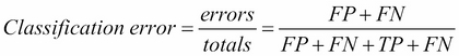
The basic two performance measures of a classifier are classification error and accuracy, as shown in the following image:

The main problem with these two measures is that they cannot handle unbalanced classes. Classifying whether a credit card transaction is an abuse or not is an example of a problem with unbalanced classes, there are 99.99% normal transactions and just a tiny percentage of abuses. Classifier that says that every transaction is a normal one is 99.99% accurate, but we are mainly interested in those few classifications that occur very rarely.
The solution is to use measures that don't involve TN (correct rejections). Two such measures are as follows:


It is common to combine the two and report the F-measure, which considers both precision and recall to calculate the score as a weighted average, where the score reaches its best value at 1 and worst at 0, as follows:

Most classification algorithms return a classification confidence denoted as f(X), which is, in turn, used to calculate the prediction. Following the credit card abuse example, a rule might look similar to the following:

The threshold determines the error rate and the true positive rate. The outcomes for all the possible threshold values can be plotted as a Receiver Operating Characteristics (ROC) as shown in the following diagram:

A random predictor is plotted with a red dashed line and a perfect predictor is plotted with a green dashed line. To compare whether the A classifier is better than C, we compare the area under the curve.
Most of the toolboxes provide all of the previous measures out-of-the-box.
Regression deals with continuous target variable, unlike classification, which works with a discrete target variable. For example, in order to forecast the outside temperature of the following few days, we will use regression; while classification will be used to predict whether it will rain or not. Generally speaking, regression is a process that estimates the relationship among features, that is, how varying a feature changes the target variable.
The most basic regression model assumes linear dependency between features and target variable. The model is often fitted using least squares approach, that is, the best model minimizes the squares of the errors. In many cases, linear regression is not able to model complex relations, for example, the next figure shows four different sets of points having the same linear regression line: the upper-left model captures the general trend and can be considered as a proper model, the bottom-left model fits points much better, except an outlier—this should be carefully checked—and the upper and lower-right side linear models completely miss the underlying structure of the data and cannot be considered as proper models.

In regression, we predict numbers Y from inputs X and the predictions are usually wrong and not exact. The main question that we ask is by how much? In other words, we want to measure the distance between the predicted and true values.
Mean squared error is an average of the squared difference between the predicted and true values, as follows:

The measure is very sensitive to the outliers, for example, 99 exact predictions and one predicton off by 10 is scored the same as all predictions wrong by 1. Moreover, the measure is sensitive to the mean. Therefore, relative squared error, which compares the MSE of our predictor to the MSE of the mean predictor (which always predicts the mean value) is often used instead.
Mean absolute error is an average of the absolute difference between the predicted and the true values, as follows:

The MAS is less sensitive to the outliers, but it is also sensitive to the mean and scale.
Correlation coefficient compares the average of prediction relative to the mean multiplied by training values relative to the mean. If the number is negative, it means weak correlation, positive number means strong correlation, and zero means no correlation. The correlation between true values X and predictions Y is defined as follows:

The CC measure is completely insensitive to the mean and scale, and less sensitive to the outliers. It is able to capture the relative ordering, which makes it useful to rank the tasks such as document relevance and gene expression.