We will now introduce two new tools that were used in the experiments for this chapter: SMILE and Elki. SMILE features a Java API that was used to illustrate feature reduction using PCA, Random Projection, and IsoMap. Subsequently, the graphical interface of Elki was used to perform unsupervised learning—specifically, clustering and outlier detection. Elki comes with a rich set of algorithms for cluster analysis and outlier detection including a large number of model evaluators to choose from.

Character-recognition is a problem that occurs in many business areas, for example, the translation of medical reports and hospital charts, postal code recognition in the postal service, check deposit service in retail banking, and others. Human handwriting can vary widely among individuals. Here, we are looking exclusively at handwritten digits, 0 to 9. The problem is made interesting due to the verisimilitude within certain sets of digits, such as 1/2/7 and 6/9/0. In our experiments in this chapter we use clustering and outlier analysis using several different algorithms to illustrate the relative strengths and weaknesses of the methods. Given the widespread use of these techniques in data mining applications, our main focus is to gain insights into the data and the algorithms and evaluation measures; we do not apply the models for prediction on test data.

As suggested by the title of the chapter, our experiments aim to demonstrate Unsupervised Learning by ignoring the labels identifying the digits in the dataset. Having learned from the dataset, clustering and outlier analyses can yield invaluable information for describing patterns in the data, and are often used to explore these patterns and inter-relationships in the data, and not just to predict the class of unseen data. In the experiments described here, we are concerned with description and exploration rather than prediction. Labels are used when available by external evaluation measures, as they are in these experiments as well.

This is already done for us. For details on how the data was collected, see: The MNIST database: http://yann.lecun.com/exdb/mnist/.

Each feature in a data point is the greyscale value of one of 784 pixels. Consequently, the type of all features is numeric; there are no categorical types except for the class attribute, which is a numeral in the range 0-9. Moreover, there are no missing data elements in the dataset. Here is a table with some basic statistics for a few pixels. The images are pre-centred in the 28 x 28 box so in most examples, the data along the borders of the box are zeros:

The Mixed National Institute of Standards and Technology (MNIST) dataset is a widely used dataset for evaluating unsupervised learning methods. The MNIST dataset is mainly chosen because the clusters in high dimensional data are not well separated.

The original MNIST dataset had black and white images from NIST. They were normalized to fit in a 20 x 20 pixel box while maintaining the aspect ratio. The images were centered in a 28 x 28 image by computing the center of mass and translating it to position it at the center of the 28 x 28 dimension grid.

Each pixel is in a range from 0 to 255 based on the intensity. The 784 pixel values are flattened out and become a high dimensional feature set for each image. The following figure depicts a sample digit 3 from the data, with mapping to the grid where each pixel has an integer value from 0 to 255.

The experiments described in this section are intended to show the application of unsupervised learning techniques to a well-known dataset. As was done in Chapter 2, Practical Approach to Real-World Supervised Learning with supervised learning techniques, multiple experiments were carried out using several clustering and outlier methods. Results from experiments with and without feature reduction are presented for each of the selected methods followed by an analysis of the results.

Since our focus is on exploring the dataset using various unsupervised techniques and not on the predictive aspect, we are not concerned with train, validation, and test samples here. Instead, we use the entire dataset to train the models to perform clustering analysis.

In the case of outlier detection, we create a reduced sample of only two classes of data, namely, 1 and 7. The choice of a dataset with two similarly shaped digits was made in order to set up a problem space in which the discriminating power of the various anomaly detection techniques would stand out in greater relief.

We demonstrate different feature analysis and dimensionality reduction methods—PCA, Random Projection, and IsoMap—using the Java API of the SMILE machine learning toolkit.

Figure 8: Showing digit 3 with pixel values distributed in a 28 by 28 matrix ranging from 0 to 254.

The code for loading the dataset and reading the values is given here along with inline comments:

//parser to parse the tab delimited file
DelimitedTextParser parser = new DelimitedTextParser();parser.setDelimiter("[	]+");
//parse the file from the location
parser.parse("mnistData", new File(fileLocation);
//the header data file has column names to map
parser.setColumnNames(true);
//the class attribute or the response variable index
AttributeDataSet dataset = parser.setResponseIndex(new NominalAttribute("class"), 784);

//convert the data into two-dimensional array for using various techniques 
double[][] data = dataset.toArray(new double[dataset.size()][]);

PCA

The following snippet illustrates dimensionality reduction achieved using the API for PCA support:

//perform PCA with double data and using covariance //matrix
PCA pca = new PCA(data, true);
//set the projection dimension as two (for plotting here)
pca.setProjection(2);
//get the new projected data in the dimension
double[][] y = pca.project(data);

Figure 9: PCA on MNIST – On the left, we see that over 90 percent of variance in data is accounted for by fewer than half the original number of features; on the right, a representation of the data using the first two principal components.

Table 2: Summary of set of 11 random features after PCA

The PCA computation reduces the number of features to 274. In the following table you can see basic statistics for a randomly selected set of features. Feature data has been normalized as part of the PCA:

Features	Average	Std Dev	Min	Max
1	0	2.982922	-35.0821	19.73339
2	0	2.415088	-32.6218	31.63361
3	0	2.165878	-21.4073	16.50271
4	0	1.78834	-27.537	31.52653
5	0	1.652688	-21.4661	22.62837
6	0	1.231167	-15.157	10.19708
7	0	0.861705	-6.04737	7.220233
8	0	0.631403	-6.80167	3.633182
9	0	0.606252	-5.46206	4.118598
10	0	0.578355	-4.21456	3.621186
11	0	0.528816	-3.48564	3.896156

Table 2: Summary of set of 11 random features after PCA

Random projections

Here, we illustrate the straightforward usage of the API for performing data transformation using random projection:

//random projection done on the data with projection in //2 dimension
RandomProjection rp = new RandomProjection(data.length, 2, false);
//get the transformed data for plotting
double[][] projectedData = rp.project(data);

Figure 10: PCA and Random projection - representations in two dimensions using Smile API

ISOMAP

This code snippet illustrates use of the API for Isomap transformation:

//perform isomap transformation of data, here in 2 //dimensions with k=10
IsoMap isomap = new IsoMap(data, 2, 10);
//get the transformed data back
double[][] y = isomap.getCoordinates();

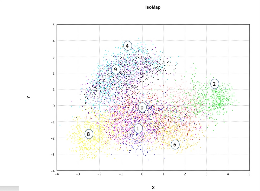
Figure 11: IsoMap – representation in two dimensions with k = 10 using Smile API

Two sets of experiments were conducted using the MNIST-6000 dataset. The dataset consists of 6,000 examples, each of which represents a hand-written digit as greyscale values of a 28 x 28 square of pixels.

First, we run some clustering techniques to identify the 10 clusters of digits. For the experiments in this part of the case study, we use the software Elki.

In the first set of experiments, there is no feature-reduction involved. All 28x28 pixels are used. Clustering techniques including k-Means, EM (Diagonal Gaussian Model Factory), DBSCAN, Hierarchical (HDBSCAN Hierarchy Extraction), as well as Affinity Propagation were used. In each case, we use metrics from two internal evaluators: Davies Bouldin and Silhouette, and several external evaluators: Precision, Recall, F1 measure, and Rand Index.

Figure 12: K-Means – using Sum of Squared Errors (SSE) to find optimal k, the number of clusters. An elbow in the curve, which is typically used to pick the optimal k value, is not particularly detectable in the plot.

In the case of k-Means, we did several runs using a range of k values. The plot shows that the Sum of Squared Errors (SSE) metric decreases with k.

The table shows results for k=10 and ranks for each are in parentheses:

In the second clustering experiment, the dataset was first pre-processed using PCA, and the resulting data with 273 features per example was used with the same algorithms as in the first experiment. The results are shown in the table:

For the outlier detection techniques, we used a subset of the original dataset containing all examples of digit 1 and an under-sampled subset of digit 7 examples. The idea is that the similarity in shape of the two digits would cause the digit 7 examples to be found to be outliers.

The models used were selected from Angular, Distance-based, clustering, LOF, and One-Class SVM.

The outlier metrics used in the evaluation were ROC AUC, Average Precision, R-Precision, and Maximum F1 measure.

The following table shows the results obtained, with ranks in parentheses: