
In real-world problems, there are many constraints on learning and many ways to assess model performance on unseen data. Each modeling algorithm has its strengths and weaknesses when applied to a given problem or to a class of problems in a particular domain. This is articulated in the famous No Free Lunch Theorem (NFLT), which says—for the case of supervised learning—that averaged over all distributions of data, every classification algorithm performs about as well as any other, including one that always picks the same class! Application of NFLT to supervised learning and search and optimization can be found at http://www.no-free-lunch.org/.
In this section, we will discuss the most commonly used practical algorithms, giving the necessary details to answer questions such as what are the algorithm's inputs and outputs? How does it work? What are the advantages and limitations to consider while choosing the algorithm? For each model, we will include sample code and outputs obtained from testing the model on the chosen dataset. This should provide the reader with insights into the process. Some algorithms such as neural networks and deep learning, Bayesian networks, stream-based earning, and so on, will be covered separately in their own chapters.
Linear models work well when the data is linearly separable. This should always be the first thing to establish.
Linear Regression can be used for both classification and estimation problems. It is one of the most widely used methods in practice. It consists of finding the best-fitting hyperplane through the data points.
Features must be numeric. Categorical features are transformed using various pre-processing techniques, as when a categorical value becomes a feature with 1 and 0 values. Linear Regression models output a categorical class in classification or numeric values in regression. Many implementations also give confidence values.
The model tries to learn a "hyperplane" in the input space that minimizes the error between the data points of each class (References [4]).
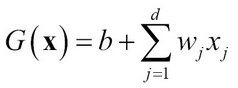
A hyperplane in d-dimensional inputs that linear model learns is given by:

The two regions (binary classification) the model divides the input space into are ![]() and
and ![]() . Associating a value of 1 to the coordinate of feature 0, that is, x0=1, the vector representation of hypothesis space or the model is:
. Associating a value of 1 to the coordinate of feature 0, that is, x0=1, the vector representation of hypothesis space or the model is:

The weight matrix can be derived using various methods such as ordinary least squares or iterative methods using matrix notation as follows:

Here X is the input matrix and y is the label. If the matrix XTX in the least squares problem is not of full rank or if encountering various numerical stability issues, the solution is modified as:

Here, ![]() is added to the diagonal of an identity matrix In of size (n + 1, n + 1) with the rest of the values being set to 0. This solution is called ridge regression and parameter λ theoretically controls the trade-off between the square loss and low norm of the solution. The constant λ is also known as regularization constant and helps in preventing "overfitting".
is added to the diagonal of an identity matrix In of size (n + 1, n + 1) with the rest of the values being set to 0. This solution is called ridge regression and parameter λ theoretically controls the trade-off between the square loss and low norm of the solution. The constant λ is also known as regularization constant and helps in preventing "overfitting".
- It is an appropriate method to try and get insights when there are less than 100 features and a few thousand data points.
- Interpretable to some level as the weights give insights on the impact of each feature.
- Assumes linear relationship, additive and uncorrelated features, hence it doesn't model complex non-linear real-world data. Some implementations of Linear Regression allow removing collinear features to overcome this issue.
- Very susceptible to outliers in the data, if there are huge outliers, they have to be treated prior to performing Linear Regression.
- Heteroskedasticity, that is, unequal training point variances, can affect the simple least square regression models. Techniques such as weighted least squares are employed to overcome this situation.
Based on the Bayes rule, the Naïve Bayes classifier assumes the features of the data are independent of each other (References [9]). It is especially suited for large datasets and frequently performs better than other, more elaborate techniques, despite its naïve assumption of feature independence.
The Naïve Bayes model can take features that are both categorical and continuous. Generally, the performance of Naïve Bayes models improves if the continuous features are discretized in the right format. Naïve Bayes outputs the class and the probability score for all class values, making it a good classifier for scoring models.
It is a probability-based modeling algorithm. The basic idea is using Bayes' rule and measuring the probabilities of different terms, as given here. Measuring probabilities can be done either using pre-processing such as discretization, assuming a certain distribution, or, given enough data, mapping the distribution for numeric features.
Bayes' rule is applied to get the posterior probability as predictions and k represents kth class.:


- It is robust against isolated noisy data points because such points are averaged when estimating the probabilities of input data.
- Probabilistic scores as confidence values from Bayes classification can be used as scoring models.
- Can handle missing values very well as they are not used in estimating probabilities.
- Also, it is robust against irrelevant attributes. If the features are not useful the probability distribution for the classes will be uniform and will cancel itself out.
- Very good in training speed and memory, it can be parallelized as each computation of probability in the equation is independent of the other.
- Correlated features can be a big issue when using Naïve Bayes because the conditional independence assumption is no longer valid.
- Normal distribution of errors is an assumption in most optimization algorithms.
If we employ Linear Regression model using, say, the least squares regression method, the outputs have to be converted to classes, say 0 and 1. Many Linear Regression algorithms output class and confidence as probability. As a rule of thumb, if we see that the probabilities of Linear Regression are mostly beyond the ranges of 0.2 to 0.8, then logistic regression algorithm may be a better choice.
Similar to Linear Regression, all features must be numeric. Categorical features have to be transformed to numeric. Like in Naïve Bayes, this algorithm outputs class and probability for each class and can be used as a scoring model.
Logistic regression models the posterior probabilities of classes using linear functions in the input features.
The logistic regression model for a binary classification is given as:

The model is a log-odds or logit transformation of linear models (References [6]). The weight vector is generally computed using various optimization methods such as iterative reweighted least squares (IRLS) or the Broyden–Fletcher–Goldfarb–Shanno (BFGS) method, or variants of these methods.
- Overcomes the issue of heteroskedasticity and some non-linearity between inputs and outputs.
- No need of normal distribution assumptions in the error estimates.
- It is interpretable, but less so than Linear Regression models as some understanding of statistics is required. It gives information such as odds ratio, p values, and so on, which are useful in understanding the effects of features on the classes as well as doing implicit feature relevance based on significance of p values.
- L1 or L2 regularization has to be employed in practice to overcome overfitting in the logistic regression models.
- Many optimization algorithms are available for improving speed of training and robustness.
Next, we will discuss some of the well-known, practical, and most commonly used non-linear models.
Decision Trees are also known as Classification and Regression Trees (CART) (References [5]). Their representation is a binary tree constructed by evaluating an inequality in terms of a single attribute at each internal node, with each leaf-node corresponding to the output value or class resulting from the decisions in the path leading to it. When a new input is provided, the output is predicted by traversing the tree starting at the root.
Features can be both categorical and numeric. It generates class as an output and most implementations give a score or probability using frequency-based estimation. Decision Trees probabilities are not smooth functions like Naïve Bayes and Logistic Regression, though there are extensions that are.
Generally, a single tree is created, starting with single features at the root with decisions split into branches based on the values of the features while at the leaf there is either a class or more features. There are many choices to be made, such as how many trees, how to choose features at the root level or at subsequent leaf level, and how to split the feature values when not categorical. This has resulted in many different algorithms or modifications to the basic Decision Tree. Many techniques to split the feature values are similar to what was discussed in the section on discretization. Generally, some form of pruning is applied to reduce the size of the tree, which helps in addressing overfitting.
Gini index is another popular technique used to split the features. Gini index of data in set S of all the data points is ![]() where p1, p2 … pk are probability distribution for each class.
where p1, p2 … pk are probability distribution for each class.
If p is the fraction or probability of data in set S of all the data points belonging to say class positive, then 1 – p is the fraction for the other class or the error rate in binary classification. If the dataset S is split in r ways S1, S2, …Sr then the error rate of each set can be quantified as |Si|. Gini index for an r way split is as follows:

The split with the lowest Gini index is used for selection. The CART algorithm, a popular Decision Tree algorithm, uses Gini index for split criteria.
The entropy of the set of data points S can similarly be computed as:

Similarly, entropy-based split is computed as:

The lower the value of the entropy split, the better the feature, and this is used in ID3 and C4.5 Decision Tree algorithms (References [12]).
The stopping criteria and pruning criteria are related. The idea behind stopping the growth of the tree early or pruning is to reduce the "overfitting" and it works similar to regularization in linear and logistic models. Normally, the training set is divided into tree growing sets and pruning sets so that pruning uses different data to overcome any biases from the growing set. Minimum Description Length (MDL), which penalizes the complexity of the tree based on number of nodes is a popular methodology used in many Decision Tree algorithms.

Figure 5: Shows a two-dimensional binary classification problem and a Decision Tree induced using splits at thresholds X1t and X1t, respectively
- The main advantages of Decision Trees are they are quite easily interpretable. They can be understood in layman's terms and are especially suited for business domain experts to easily understand the exact model.
- If there are a large number of features, then building Decision Tree can take lots of training time as the complexity of the algorithm increases.
- Decision Trees have an inherent problem with overfitting. Many tree algorithms have pruning options to reduce the effect. Using pruning and validation techniques can alleviate the problem to a large extent.
- Decision Trees work well when there is correlation between the features.
- Decision Trees build axis-parallel boundaries across classes, the bias of which can introduce errors, especially in a complex, smooth, non-linear boundary.
K-Nearest Neighbors falls under the branch of non-parametric and lazy algorithms. K-Nearest neighbors doesn't make any assumptions on the underlying data and doesn't build and generalize models from training data (References [10]).
Though KNN's can work with categorical and numeric features, the distance computation, which is the core of finding the neighbors, works better with numeric features. Normalization of numeric features to be in the same ranges is one of the mandatory steps required. KNN's outputs are generally the classes based on the neighbors' distance calculation.
KNN uses the entire training data to make predictions on unseen test data. When unseen test data is presented KNN finds the K "nearest neighbors" using some distance computation and based on the neighbors and the metric of deciding the category it classifies the new point. If we consider two vectors represented by x1 and x2 corresponding to two data points the distance is calculated as:
- Euclidean Distance:

- Cosine Distance or similarity:

The metric used to classify an unseen may simply be the majority class among the K neighbors.
The training time is small as all it has to do is build data structures to hold the data in such a way that the computation of the nearest neighbor is minimized when unseen data is presented. The algorithm relies on choices of how the data is stored from training data points for efficiency of searching the neighbors, which distance computation is used to find the nearest neighbor, and which metrics are used to categorize based on classes of all neighbors. Choosing the value of "K" in KNN by using validation techniques is critical.

Figure 6: K-Nearest Neighbor illustrated using two-dimensional data with different choices of k.
- No assumption on underlying data distribution and minimal training time makes it a very attractive method for learning.
- KNN uses local information for computing the distances and in certain domains can yield highly adaptive behaviors.
- It is robust to noisy training data when K is effectively chosen.
- Holding the entire training data for classification can be problematic depending on the number of data points and hardware constraints
- Number of features and the curse of dimensionality affects this algorithm more hence some form of dimensionality reduction or feature selection has to be done prior to modeling in KNN.
SVMs, in simple terms, can be viewed as linear classifiers that maximize the margin between the separating hyperplane and the data by solving a constrained optimization problem. SVMs can even deal with data that is not linearly separable by invoking transformation to a higher dimensional space using kernels described later.
SVM is effective with numeric features only, though most implementations can handle categorical features with transformation to numeric or binary. Normalization is often a choice as it helps the optimization part of the training. Outputs of SVM are class predictions. There are implementations that give probability estimates as confidences, but this requires considerable training time as they use k-fold cross-validation to build the estimates.
In its linear form, SVM works similar to Linear Regression classifier, where a linear decision boundary is drawn between the two classes. The difference between the two is that with SVM, the boundary is drawn in such a way that the "margin" or the distance between the points near the boundary is maximized. The points on the boundaries are known as "support vectors" (References [13 and 8]).
Thus, SVM tries to find the weight vector in linear models similar to Linear Regression model as given by the following:
The weight w0 is represented by b here. SVM for a binary class y ∈{1,-1} tries to find a hyperplane:

The hyperplane tries to separate the data points such that all points with the class lie on the side of the hyperplane as:


The models are subjected to maximize the margin using constraint-based optimization with a penalty function denoted by C for overcoming the errors denoted by ![]() :
:

Such that ![]() and
and ![]() .
.
They are also known as large margin classifiers for the preceding reason. The kernel-based SVM transforms the input data into a hypothetical feature space where SV machinery works in a linear way and the boundaries are drawn in the feature spaces.
A kernel function on the transformed representation is given by:

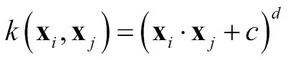
Here Φ is a transformation on the input space. It can be seen that the entire optimization and solution of SVM remains the same with the only exception that the dot-product xi · xj is replaced by the kernel function k(xi, xj), which is a function involving the two vectors in a different space without actually transforming to that space. This is known as the kernel trick.
The most well-known kernels that are normally used are:
- Gaussian Radial Basis Kernel:

- Polynomial Kernel:
- Sigmoid Kernel:

SVM's performance is very sensitive to some of the parameters of optimization and the kernel parameters and the core SV parameter such as the cost function C. Search techniques such as grid search or evolutionary search combined with validation techniques such as cross-validation are generally used to find the best parameter values.

Figure 7: SVM Linear Hyperplane learned from training data that creates a maximum margin separation between two classes.

Figure 8: Kernel transformation illustrating how two-dimensional input space can be transformed using a polynomial transformation into a three-dimensional feature space where data is linearly separable.
- SVMs are among the best in generalization, low overfitting, and have a good theoretical foundation for complex non-linear data if the parameters are chosen judiciously.
- SVMs work well even with a large number of features and less training data.
- SVMs are less sensitive to noisy training data.
- The biggest disadvantage of SVMs is that they are not interpretable.
- Another big issue with SVM is its training time and memory requirements. They are O(n2) and O(n3) and can result in major scalability issues when the data is large or there are hardware constraints. There are some modifications that help in reducing both.
- SVM generally works well for binary classification problems, but for multiclass classification problems, though there are techniques such as one versus many and one versus all, it is not as robust as some other classifiers such as Decision Trees.
Combining multiple algorithms or models to classify instead of relying on just one is known as ensemble learning. It helps to combine various models as each model can be considered—at a high level—as an expert in detecting specific patterns in the whole dataset. Each base learner can be made to learn on slightly different datasets too. Finally, the results from all models are combined to perform prediction. Based on how similar the algorithms used in combination are, how the training dataset is presented to each algorithm, and how the algorithms combine the results to finally classify the unseen dataset, there are many branches of ensemble learning:

Figure 9: Illustration of ensemble learning strategies
Some common types of ensemble learning are:
- Different learning algorithms
- Same learning algorithms, but with different parameter choices
- Different learning algorithms on different feature sets
- Different learning algorithms with different training data
It is one of the most commonly used ensemble methods for dividing the data in different samples and building classifiers on each sample.
The input is constrained by the choice of the base learner used—if using Decision Trees there are basically no restrictions. The method outputs class membership along with the probability distribution for classes.
The core idea of bagging is to apply the bootstrapping estimation to different learners that have high variance, such as Decision Trees. Bootstrapping is any statistical measure that depends on random sampling with replacement. The entire data is split into different samples using bootstrapping and for each sample, a model is built using the base learner. Finally, while predicting, the average prediction is arrived at using a majority vote—this is one technique to combine over all the learners.
Random Forest is an improvement over basic bagged Decision Trees. Even with bagging, the basic Decision Tree has a choice of all the features at every split point in creating a tree. Because of this, even with different samples, many trees can form highly correlated submodels, which causes the performance of bagging to deteriorate. By giving random features to different models in addition to a random dataset, the correlation between the submodels reduces and Random Forest shows much better performance compared to basic bagged trees. Each tree in Random Forest grows its structure on the random features, thereby minimizing the bias; combining many such trees on decision reduces the variance (References [15]). Random Forest is also used to measure feature relevance by averaging the impurity decrease in the trees and ranking them across all the features to give the relative importance of each.
- Better generalization than the single base learner. Overcomes the issue of overfitting of base learners.
- Interpretability of bagging is very low as it works as meta learner combining even the interpretable learners.
- Like most other ensemble learners, Bagging is resilient to noise and outliers.
- Random Forest generally does not tend to overfit given the training data is iid.
Boosting is another popular form of ensemble learning, which is based on using a weak learner and iteratively learning the points that are "misclassified" or difficult to learn. Thus, the idea is to "boost" the difficult to learn instances and making the base learners learn the decision boundaries more effectively. There are various flavors of boosting such as AdaBoost, LogitBoost, ConfidenceBoost, Gradient Boosting, and so on. We present a very basic form of AdaBoost here (References [14]).
The input is constrained by the choice of the base learner used—if using Decision Trees there are basically no restrictions. Outputs class membership along with probability distribution for classes.
The basic idea behind boosting is iterative reweighting of input samples to create new distribution of the data for learning a model from a simple base learner in every iteration.
Initially, all the instances are uniformly weighted with weights  and at every iteration t, the population is resampled or reweighted as
  where
where  and Zt is the normalization constant.
The final model works as a linear combination of all the models learned in the iteration:

The reweighting or resampling of the data in each iteration is based on "errors"; the data points that result in errors are sampled more or have larger weights.
- Better generalization than the base learner and overcomes the issue of overfitting very effectively.
- Some boosting algorithms such as AdaBoost can be susceptible to uniform noise. There are variants of boosting such as "GentleBoost" and "BrownBoost" that decrease the effect of outliers.
- Boosting has a theoretical bounds and guarantee on the error estimation making it a statistically robust algorithm.