
The key ideas discussed here are:
In order to train the model(s), tune the model parameters, select the models, and finally estimate the predictive behavior of models on unseen data, we need many datasets. We cannot train the model on one set of data and estimate its behavior on the same set of data, as it will have a clear optimistic bias and estimations will be unlikely to match the behavior in the unseen data. So at a minimum, there is a need to partition data available into training sets and testing sets. Also, we need to tune the parameters of the model and test the effect of the tuning on a separate dataset before we perform testing on the test set. The same argument of optimistic bias and wrong estimation applies if we use the same dataset for training, parameter tuning, and testing. Thus there is a theoretical and practical need to have three datasets, that is, training, validation, and testing.
The models are trained on the training set, the effect of different parameters on the training set are validated on the validation set, and the finalized model with the selected parameters is run on the test set to gauge the performance of the model on future unseen data. When the dataset is not large enough, or is large but the imbalance between classes is wide, that is, one class is present only in a small fraction of the total population, we cannot create too many samples. Recall that one of the steps described in our methodology is to create different data samples and datasets. If the total training data is large and has a good proportion of data and class ratios, then creating these three sets using random stratified partitioning is the most common option employed. In certain datasets that show seasonality and time-dependent behaviors, creating datasets based on time bounds is a common practice. In many cases, when the dataset is not large enough, only two physical partitions, that is, training and testing may be created. The training dataset ranges roughly from 66% to 80% while the rest is used for testing. The validation set is then created from the training dataset using the k-fold cross-validation technique. The training dataset is split k times, each time producing k-1/k random training 1/k testing data samples, and the average metrics of performance needed is generated. This way the limited training data is partitioned k times and average performance across different split of training/testing is used for gauging the effect of the parameters. Using 10-fold cross-validation is the most common practice employed in cross-validation.
The next important decision when tuning parameters or selecting models is to base your decision on certain performance metrics. In classification learning, there are different metrics available on which you can base your decision, depending on the business requirement. For example, in certain domains, not missing a single true positive is the most important concern, while in other domains where humans are involved in adjudicating results of models, having too many false positives is the greater concern. In certain cases, having overall good accuracy is considered more vital. In highly imbalanced datasets such as fraud or cyber attacks, there are just a handful of instances of one class and millions of the other classes. In such cases accuracy gives a wrong indication of model performance and some other metrics such as precision, true positive ratio, or area under the curve are used as metrics.
We will now discuss the most commonly employed metrics in classification algorithms evaluation (References [16, 17, and 19]).

Figure 10: Model evaluation metrics for classification models

Figure 11: Confusion Matrix
The confusion matrix is central to the definition of a number of model performance metrics. The proliferation of metrics and synonymous terms is a result of the utility of different quantities derived from the elements of the matrix in various disciplines, each emphasizing a different aspect of the model's behavior.
The four elements of the matrix are raw counts of the number of False Positives, False Negatives, True Positives, and True Negatives. Often more interesting are the different ratios of these quantities, the True Positive Rate (or Sensitivity, or Recall), and the False Positive Rate (FPR, or 1—Specificity, or Fallout). Accuracy reflects the percentage of correct predictions, whether Class 1 or Class 0. For skewed datasets, accuracy is not particularly useful, as even a constant prediction can appear to perform well.
The previously mentioned metrics such as accuracy, precision, recall, sensitivity, and specificity are aggregates, that is, they describe the behavior of the entire dataset. In many complex problems it is often valuable to see the trade-off between metrics such as TPs and say FPs.
Many classifiers, mostly probability-based classifiers, give confidence or probability of the prediction, in addition to giving classification. The process to obtain the ROC or PRC curves is to run the unseen validation or test set on the learned models, and then obtain the prediction and the probability of prediction. Sort the predictions based on the confidences in decreasing order. For every probability or confidence calculate two metrics, the fraction of FP (FP rate) and the fraction of TP (TP rate).
Plotting the TP rate on the y axis and FP rate on the x axis gives the ROC curves. ROC curves of random classifiers lie close to the diagonal while the ROC curves of good classifiers tend towards the upper left of the plot. The area under the curve (AUC) is the area measured under the ROC curve by using the trapezoidal area from 0 to 1 of ROC curves. While running cross-validation for instance there can be many ROC curves. There are two ways to get "average" ROC curves: first, using vertical averaging, that is, TPR average is plotted at different FP rate or second, using horizontal averaging, that is, FPR average is plotted at different TP rate. The classifiers that have area under curves greater than 0.8, as a rule-of-thumb are considered good for prediction for unseen data.
Precision Recall curves or PRC curves are similar to ROC curves, but instead of TPR versus FPR, metrics Precision and Recall are plotted on the y and x axis, respectively. When the data is highly imbalanced, that is, ROC curves don't really show the impact while PRC curves are more reliable in judging performance.
Lift and Gain charts are more biased towards sensitivity or true positives. The whole purpose of these two charts is to show how instead of random selection, the models prediction and confidence can detect better quality or true positives in the sample of unseen data.
This is usually very appealing for detection engines that are used in detecting fraud in financial crime or threats in cyber security. The gain charts and lift curves give exact estimates of real true positives that will be detected at different quartiles or intervals of total data. This will give insight to the business decision makers on how many investigators would be needed or how many hours would be spent towards detecting fraudulent actions or cyber attacks and thus can give real ROI of the models.
The process for generating gain charts or lift curves has a similar process of running unseen validation or test data through the models and getting the predictions along with the confidences or probabilities. It involves ranking the probabilities in decreasing order and keeping count of TPs per quartile of the dataset. Finally, the histogram of counts per quartile give the lift curve, while the cumulative count of TPs added over quartile gives the gains chart. In many tools such as RapidMiner, instead of coarse intervals such as quartiles, fixed larger intervals using binning is employed for obtaining the counts and cumulative counts.
When it comes to choosing between algorithms, or the right parameters for a given algorithm, we make the comparison either on different datasets, or, as in the case of cross-validation, on different splits of the same dataset. Measures of statistical testing are employed in decisions involved in these comparisons. The basic idea of using hypothesis testing from classical statistics is to compare the two metrics from the algorithms. The null hypothesis is that there is no difference between the algorithms based on the measured metrics and so the test is done to validate or reject the null hypothesis based on the measured metrics (References [16]). The main question answered by statistical tests is- are the results or metrics obtained by the algorithm its real characteristics, or is it by chance?
In this section, we will discuss the most common methods for comparing classification algorithms used in practical scenarios.
The general process is to train the algorithms on the same training set and run the models on either multiple validation sets, different test sets, or cross-validation, gauge the metrics of interest discussed previously, such as error rate or area under curve, and then get the statistics of the metrics for each of the algorithms to decide which worked better. Each method has its advantages and disadvantages.
This is a non-parametric test and thus it makes no assumptions on data and distribution. McNemar's test builds a contingency table of a performance metric such as "misclassification or errors" with:
Count of misclassification by both algorithms (c00)
- Count of misclassification by algorithm G1, but correctly classified by algorithm G2(c01)
- Count of misclassification by algorithm G2, but correctly classified by algorithm G1 (c10)
- Count of correctly classified by both G1 and G2(c11)

If χ2 exceeds ![]() statistic then we can reject the null hypothesis that the two performance metrics on algorithms G1 and G2 were equal under the confidence value of 1 – α.
statistic then we can reject the null hypothesis that the two performance metrics on algorithms G1 and G2 were equal under the confidence value of 1 – α.
This is a parametric test and an assumption of normally distributed computed metrics becomes valid. Normally it is coupled with cross-validation processes and results of metrics such as area under curve or precision or error rate is computed for each and then the mean and standard deviations are measured. Apart from normal distribution assumption, the additional assumption that two metrics come from a population of equal variance can be a big disadvantage for this method.

![]() is difference of means in performance metrics of two algorithms G1 and G2.
is difference of means in performance metrics of two algorithms G1 and G2.

Here, di is the difference between the performance metrics of two algorithms G1 and G2 in the trial and there are n trials.
The t-statistic is computed using the mean differences and the standard errors from the standard deviation as follows and is compared to the table for the right alpha value to check for significance:

The most popular non-parametric method of testing two metrics over datasets is to use the Wilcoxon signed-rank test. The algorithms are trained on the same training data and metrics such as error rate or area under accuracy are calculated over different validation or test sets. Let di be the difference between the performance metrics of two classifiers in the ith trial for N datasets. Differences are then ranked according to their absolute values, and mean ranks associated for ties. Let R+ be the sum of ranks where the second algorithm outperformed the first and R– be the sum of ranks where the first outperformed the second:


The statistic ![]() is then compared to threshold value at an alpha,
is then compared to threshold value at an alpha, ![]() to reject the hypothesis.
to reject the hypothesis.
We will now discuss the two most common techniques used when there are more than two algorithms involved and we need to perform comparison across many algorithms for evaluation metrics.
These are parametric tests that assume normal distribution of the samples, that is, metrics we are calculating for evaluations. ANOVA test follows the same process as others, that is, train the models/algorithms on similar training sets and run it on different validation or test sets. The main quantities computed in ANOVA are the metric means for each algorithm performance and then compute the overall metric means across all algorithms.
Let pij be the performance metric for i = 1,2… k and j = 1,2 …l for k trials and l classifiers. The mean performance of classifier j on all trials and overall mean performance is:


Two types of variation are evaluated. The first is within-group variation, that is, total deviation of each algorithm from the overall metric mean, and the second is between-group variation, that is, deviation of each algorithm metric mean. Within-group variation and between-group variation are used to compute the respective within- and between- sum of squares as:

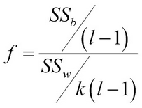
Using the two sum of squares and a computation such as F-statistic, which is the ratio of the two, the significance test can be done at alpha values to accept or reject the null hypothesis:
ANOVA tests have the same limitations as paired-t tests on the lines of assumptions of normal distribution of metrics and assuming the variances being equal.
Friedman's test is a non-parametric test for multiple algorithm comparisons and it has no assumption on the data distribution or variances of metrics that ANOVA does. It uses ranks instead of the performance metrics directly for its computation. On each dataset or trials, the algorithms are sorted and the best one is ranked 1 and so on for all classifiers. The average rank of an algorithm over n datasets is computed, say Rj. The Friedman's statistic over l classifiers is computed as follows and compared to alpha values to accept or reject the null hypothesis:
