
In this section, we will discuss some common preprocessing and transformation steps that are done in most text mining processes. The general concept is to convert the documents into structured datasets with features or attributes that most Machine Learning algorithms can use to perform different kinds of learning.
We will briefly describe some of the most used techniques in the next section. Different applications of text mining might use different pieces or variations of the components shown in the following figure:

Figure 10: Text Processing components and the flow
One of the first steps in most text mining applications is the collection of data in the form of a body of documents—often referred to as a corpus in the text mining world. These documents can have predefined categorization associated with them or it can simply be an unlabeled corpus. The documents can be of heterogeneous formats or standardized into one format for the next process of tokenization. Having multiple formats such as text, HTML, DOCs, PDGs, and so on, can lead to many complexities and hence one format, such as XML or JavaScript Object Notation (JSON) is normally preferred in most applications.
Inputs are vast collections of homogeneous or heterogeneous sources and outputs are a collection of documents standardized into one format, such as XML.
Standardization involves ensuring tools and formats are agreed upon based on the needs of the application:
- Agree to a standard format, such as XML, with predefined tags that provide information on meta-attributes of documents
(<author>,<title>,<date>, and so on) and actual content, such as<document>. - Most document processors can either be transformed into XML or transformation code can be written to perform this.
The task of tokenization is to extract words or meaningful characters from the text containing a stream of these words. For example, the text The boy stood up. He then ran after the dog can be tokenized into tokens such as {the, boy, stood, up, he, ran, after, the, dog}.
An input is a collection of documents in a well-known format as described in the last section and an output is a document with tokens of words or characters as needed in the application.
Any automated system for tokenization must address the particular challenges presented by the language(s) it is expected to handle:
- In languages such as English, tokenization is relatively simple due to the presence of white space, tabs, and newline for separating the words.
- There are different challenges in each language—even in English, abbreviations such as Dr., alphanumeric characters (B12), different naming schemes (O'Reilly), and so on, must be tokenized appropriately.
- Language-specific rules in the form of if-then instructions are written to extract tokens from the documents.
This involves removing high frequency words that have no discriminatory or predictive value. If every word can be viewed as a feature, this process reduces the dimension of the feature vector by a significant number. Prepositions, articles, and pronouns are some of the examples that form the stop words that are removed without affecting the performance of text mining in many applications.
An input is a collection of documents with the tokens extracted and an output is a collection of documents with tokens reduced by removing stop words.
There are various techniques that have evolved in the last few years ranging from manually precompiled lists to statistical elimination using either term-based or mutual information.
- The most commonly used technique for many languages is a manually precompiled list of stop words, including prepositions (in, for, on), articles (a, an, the), pronouns (his, her, they, their), and so on.
- Many tools use Zipf's law (References [3]), where high frequency words, singletons, and unique terms are removed. Luhn's early work (References [4]), as represented in the following figure 11, shows thresholds of the upper bound and lower bound of word frequency, which give us the significant words that can be used for modeling:

Figure 11: Word Frequency distribution, showing how frequently used, significant and rare words exist in corpus
The idea of normalizing tokens of similar words into one is known as stemming or lemmatization. Thus, reducing all occurrences of "talking", "talks", "talked", and so on in a document to one root word "talk" in the document is an example of stemming.
An input is documents with tokens and an output is documents with reduced tokens normalized to their stem or root words.
- There are basically two types of stemming: inflectional stemming and stemming to the root.
- Inflectional stemming generally involves removing affixes, normalizing the verb tenses and removing plurals. Thus, "ships" to "ship", "is", "are" and "am" to "be" in English.
- Stemming to the root is generally a more aggressive form than inflectional stemming, where words are normalized to their roots. An example of this is "applications", "applied", "reapply", and so on, all reduced to the root word "apply".
- Lovin's stemmer was one of the first stemming algorithms (References [1]). Porter's stemming, which evolved in the 1980s with around 60 rules in 6 steps, is still the most widely used form of stemming (References [2]).
- Present-day applications drive a wide range of statistical techniques based on stemming, including those using n-grams (a contiguous sequence of n items, either letters or words from a given sequence of text), hidden Markov models (HMM), and context-sensitive stemming.
Once the preprocessing task of converting documents into tokens is performed, the next step is the creation of a corpus or vocabulary as a single dictionary, using all the tokens from all documents. Alternatively, several dictionaries are created based on category, using specific tokens from fewer documents.
Many applications in topic modeling and text categorization perform well when dictionaries are created per topic/category, which is known as a local dictionary. On the other hand, many applications in document clustering and information extraction perform well when one single global dictionary is created from all the document tokens. The choice of creating one or many specific dictionaries depends on the core NLP task, as well as on computational and storage requirements.
A key step in converting the document(s) with unstructured text is to transform them into datasets with structured features, similar to what we have seen so far in Machine Learning datasets. Extracting features from text so that it can be used in Machine Learning tasks such as supervised, unsupervised, and semi-supervised learning depends on many factors, such as the goals of the applications, domain-specific requirements, and feasibility. There are a wide variety of features, such as words, phrases, sentences, POS-tagged words, typographical elements, and so on, that can be extracted from any document. We will give a broad range of features that are commonly used in different Machine Learning applications.
Lexical features are the most frequently used features in text mining applications. Lexical features form the basis for the next level of features. They are the simple character- or word- level features constructed without trying to capture information about intent or the various meanings associated with the text. Lexical features can be further broken down into character-based features, word-based features, part-of-speech features, and taxonomies, for example. In the next section, we will describe some of them in greater detail.
Individual characters (unigram) or a sequence of characters (n-gram) are the simplest forms of features that can be constructed from the text document. The bag of characters or unigram characters have no positional information, while higher order n-grams capture some amount of context and positional information. These features can be encoded or given numeric values in different ways, such as binary 0/1 values, or counts, for example, as discussed later in the next section.
Let us consider the memorable Dr. Seuss rhyme as the text content—"the Cat in the Hat steps onto the mat". While the bag-of-characters (1-gram or unigram features) will generate unique characters {"t","h", "e", "c","a","i","n","s","p","o","n","m"} as features, the 3-gram features are { "sCa" ,"sHa", "sin" , "sma", "son", "sst", "sth", "Cat", "Hat", "ats", "esC", "esH", "esm", "eps", "hes", "ins ", "mat", "nst", "nto", "ost", "ont", "pss", "sso" , "ste"," tsi"," tss" , "tep", "the", "tos "}. As can be seen, as "n" increases, the number of features increases exponentially and soon becomes unwieldy. The advantage of n-grams is that at the cost of increasing the total number of features, the assembled features often seem to capture combinations of characters that are more interesting than the individual characters themselves.
Instead of generating features from characters, features can similarly be constructed from words in a unigram and n-gram manner. These are the most popular feature generation techniques. The unigram or 1-word token is also known as the bag of words model. So the example of "the Cat in the Hat steps onto the mat" when considered as unigram features is {"the", "Cat", "in", "Hat", "steps", "onto", "mat"}. Similarly, bigram features on the same text would result in {"the Cat", "Cat in", "in the", "the Hat", "Hat step", "steps onto", "onto the", "the mat"}. As in the case of character-based features, by going to higher "n" in the n-grams, the number of features increases, but so does the ability to capture word sense via context.
The input is text with words and the output is text where every word is associated with the grammatical tag. In many applications, part-of-speech gives a context and is useful in identification of named entities, phrases, entity disambiguation, and so on. In the example "the Cat in the Hat steps onto the mat" , the output is {"theDet", "CatNoun", "inPrep", "theDet", "HatNoun", "stepsVerb", "ontoPrep", "theDet", "matNoun"}. Language specific rule-based taggers or Markov chain–based probabilistic taggers are often used in this process.
Creating taxonomies from the text data and using it to understand relationships between words is also useful in different contexts. Various taxonomical features such as hypernyms, hyponyms, is-member, member-of, is-part, part-of, antonyms, synonyms, acronyms, and so on, give lexical context that proves useful in searches, retrieval, and matching in many text mining scenarios.
The next level of features that are higher than just characters or words in text documents are the syntax-based features. Syntactical representation of sentences in text is generally in the form of syntax trees. Syntax trees capture nodes as terms used in sentences, and relationships between the nodes are captured as links. Syntactic features can also capture more complex features about sentences and usage—such as aggregates—that can be used for Machine Learning. It can also capture statistics about syntax trees—such as sentences being left-heavy, right-heavy, or balanced—that can be used to understand signatures of different content or writers.
Two sentences can have the same characters and words in the lexical analysis, but their syntax trees or intent could be completely different. Breaking the sentences in the text into different phrases—Noun Phrase (NP), Prepositional Phrase (PP), Verbal (or Gerund) Phrase (VP), and so on—and capturing phrase structure trees for the sentences are part of this processing task. The following is the syntactic parse tree for our example sentence:
(S (NP (NP the cat)
       (PP in
           (NP the hat)))
   (VP steps
       (PP onto
           (NP the mat))))
Syntactic Language Models (SLM) are about determining the probability of a sequence of terms. Language model features are used in machine translation, spelling correction, speech translation, summarization, and so on, to name a few of the applications. Language models can additionally use parse trees and syntax trees in their computation as well.
The chain rule is applied to compute the joint probability of terms in the sentence:

In the example "the cat in the hat steps onto the mat":

Generally, the estimation of the probability of long sentences based on counts using any corpus is difficult due to the need for many examples of such sentences. Most language models use the Markov assumption of independence and n-grams (2-5 words) in practical implementations (References [8]).
Semantic features attempt to capture the "meaning" of the text, which is then used for different applications of text mining. One of the simplest forms of semantic features is the process of adding annotations to the documents. These annotations, or metadata, can have additional information that describes or captures the intent of the text or documents. Adding tags using collaborative tagging to capture tags as keywords describing the text is a common semantic feature generation process.
Another form of semantic feature generation is the process of ontological representation of the text. Generic and domain specific ontologies that capture different relationships between objects are available in knowledge bases and have well-known specifications, such as Semantic Web 2.0. These ontological features help in deriving complex inferencing, summarization, classification, and clustering tasks in text mining. The terms in the text or documents can be mapped to "concepts" in ontologies and stored in knowledge bases. These concepts in ontologies have semantic properties, and are related to other concepts in a number of ways, such as generalization/specialization, member-of/isAMember, association, and so on, to name a few. These attributes or properties of concepts and relationships can be further used in search, retrieval, and even in predictive modeling. Many semantic features use the lexical and syntactic processes as pre-cursors to the semantic process and use the outputs, such as nouns, to map to concepts in ontologies, for example. Adding the concepts to an existing ontology or annotating it with more concepts makes the structure more suitable for learning. For example, in the "the cat in the .." sentence, "cat" has properties such as {age, eats, ...} and has different relationships, such as { "isA Mammal", "hasChild", "hasParent", and so on}.
Lexical, syntactic, and semantic features, described in the last section, often have representations that are completely different from each other. Representations of the same feature type, that is, lexical, syntactic, or semantic, can differ based on the computation or mining task for which they are employed. In this section, we will describe the most common lexical feature-based representation known as vector space models.
The vector space model (VSM) is a transformation of the unstructured document to a numeric vector representation where terms in the corpus form the dimensions of the vector and we use some numeric way of associating value with these dimensions.
As discussed in the section on dictionaries, a corpus is formed out of unique words and phrases from the entire collection of documents in a domain or within local sub-categories of one. Each of the elements of such a dictionary are the dimensions of the vector. The terms—which can be single words or phrases, as in n-grams—form the dimensions and can have different values associated with them in a given text/document. The goal is to capture the values in the dimensions in a way that reflects the relevancy of the term(s) in the entire corpus (References [11]). Thus, each document or file is represented as a high-dimensional numeric vector. Due to the sparsity of terms, the numeric vector representation has a sparse representation in numeric space. Next, we will give some well-known ways of associating values to these terms.
This is the simplest form of associating value to the terms, or dimensions. In binary form, each term in the corpus is given a 0 or 1 value based on the presence or absence of the term in the document. For example, consider the following three documents:
- Document 1: "The Cat in the Hat steps onto the mat"
- Document 2: "The Cat sat on the Hat"
- Document 3: "The Cat loves to step on the mat"
After preprocessing by removing stop words {on, the, in, onto} and stemming {love/loves, steps/step} using a unigram or bag of words, {cat, hat, step, mat, sat, love} are the features of the corpus. Each document is now represented in a binary vector space model as follows:
|
Terms |
cat |
hat |
step |
mat |
sat |
love |
|---|---|---|---|---|---|---|
|
Document 1 |
1 |
1 |
1 |
1 |
0 |
0 |
|
Document 2 |
1 |
1 |
0 |
0 |
1 |
0 |
|
Document 3 |
1 |
0 |
1 |
1 |
0 |
1 |
In term frequency (TF), as the name suggests, the frequency of terms in the entire document forms the numeric value of the feature. The basic assumption is that the higher the frequency of the term, the greater the relevance of that term for the document. Counts of terms or normalized counts of terms are used as values in each column of terms:
tf(t) = count(D, t)
The following table gives term frequencies for the three documents in our example:
|
TF / Terms |
cat |
hat |
step |
mat |
sat |
love |
|---|---|---|---|---|---|---|
|
Document 1 |
1 |
1 |
1 |
1 |
0 |
0 |
|
Document 2 |
1 |
1 |
0 |
0 |
1 |
0 |
|
Document 3 |
1 |
0 |
1 |
1 |
0 |
1 |
Inverse document frequency (IDF) has various flavors, but the most common way of computing it is using the following:

Here, ![]()
![]() IDF favors mostly those terms that occur relatively infrequently in the documents. Some empirically motivated improvements to IDF have also been proposed in the research (References [7]).
IDF favors mostly those terms that occur relatively infrequently in the documents. Some empirically motivated improvements to IDF have also been proposed in the research (References [7]).
TF for our example corpus:
|
Terms |
cat |
hat |
step |
mat |
sat |
love |
|---|---|---|---|---|---|---|
|
N/nj |
3/3 |
3/2 |
3/2 |
3/2 |
3/1 |
3/1 |
|
IDF |
0.0 |
0.40 |
0.40 |
0.40 |
1.10 |
1.10 |
Combining both term frequencies and inverse document frequencies in one metric, we get the term frequency-inverse document frequency values. The idea is to value those terms that are relatively uncommon in the corpus (high IDF), but are reasonably relevant for the document (high TF). TF-IDF is the most common form of value association in many text mining processes:

This gives us the TF-IDF for all the terms in each of the documents:
|
TF-IDF/Terms |
cat |
hat |
step |
mat |
sat |
love |
|---|---|---|---|---|---|---|
|
Document 1 |
0.0 |
0.40 |
0.40 |
0.40 |
1.10 |
1.10 |
|
Document 2 |
0.0 |
0.40 |
0.0 |
0.0 |
1.10 |
0.0 |
|
Document 3 |
0.0 |
0.0 |
0.40 |
0.40 |
0.0 |
1.10 |
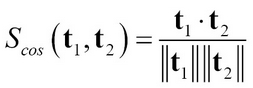
Many techniques in supervised, unsupervised, and semi-supervised learning use "similarity" measures in their underlying algorithms to find similar patterns or to separate different patterns. Similarity measures are tied closely to the representation of the data. In the VSM representation of documents, the vectors are very high dimensional and sparse. This poses a serious issue in most traditional similarity measures for classification, clustering, or information retrieval. Angle-based similarity measures, such as cosine distances or Jaccard coefficients, are more often used in practice. Consider two vectors represented by t1 and t2 corresponding to two text documents.

This angle-based similarity measure considers orientation between vectors only and not their lengths. It is equal to the cosine of the angle between the vectors. Since the vector space model is a positive space, cosine distance varies from 0 (orthogonal, no common terms) to 1 (all terms are common to both, but not necessarily with the same term frequency):
This measure the distance in a reduced feature space by only considering the features that are most important in the two documents:

Here, ti,k is a vector formed from a subset of the features of ti (i = 1, 2) containing the union of the K largest features appearing in t1 and t2.


The goal is the same as in Chapter 2, Practical Approach to Real-World Supervised Learning and Chapter 3, Unsupervised Machine Learning Techniques. The problem of the curse of dimensionality becomes even more pronounced with text mining and high dimensional features.
Most feature selection techniques are supervised techniques that depend on the labels or the outcomes for scoring the features. In the majority of cases, we perform filter-based rather than wrapper-based feature selection, due to the lower performance cost. Even among filter-based methods, some, such as those involving multivariate techniques such as Correlation based Feature selection (CFS), as described in Chapter 2, Practical Approach to Real-World Supervised Learning, can be quite costly or result in suboptimal performance due to high dimensionality (References [9]).
As shown in Chapter 2, Practical Approach to Real-World Supervised Learning, filter-based univariate feature selection methods, such as Information gain (IG) and Gain Ratio (GR), are most commonly used once preprocessing and feature extraction is done.
In their research, Yang and Pederson (References [10]) clearly showed the benefits of feature selection and reduction using IG to remove close to 98% of terms and yet improve the predictive capability of the classifiers.
Many of the information theoretic or entropy-based methods have a stronger influence resulting from the marginal probabilities of the tokens. This can be an issue when the terms have equal conditional probability P(t|class), the rarer terms may have better scores than the common terms.
?2 feature selection is one of the most common statistical-based techniques employed to perform feature selection in text mining. ?2 statistics, as shown in Chapter 2, Practical Approach to Real-World Supervised Learning, give the independence relationship between the tokens in the text and the classes.
It has been shown that ?2 statistics for feature selection may not be effective when there are low-frequency terms (References [19]).
Using the term frequency or the document frequency described in the section on feature representation, a threshold can be manually set, and only terms above or below a certain threshold can be allowed used for modeling in either classification or clustering tasks. Note that term frequency (TF) and document frequency (DF) methods are biased towards common words while some of the information theoretic or statistical-based methods are biased towards less frequent words. The choice of selection of features depends on the domain, the particular application of predictive learning, and more importantly, on how models using these features are evaluated, especially on the unseen dataset.
Another approach that we saw in Chapter 3, Unsupervised Machine Learning Techniques, was to use unsupervised techniques to reduce the features using some form of transformation to decide their usefulness.
Principal component analysis (PCA) computes a covariance or correlation matrix from the document-term matrix. It transforms the data into linear combinations of terms in the inputs in such a way that the transformed combination of features or terms has higher discriminating power than the input terms. PCA with cut-off or thresholding on the transformed features, as shown in Chapter 3, Unsupervised Machine Learning Techniques, can bring down the dimensionality substantially and even improve or give comparable performance to the high dimensional input space. The only issue with using PCA is that the transformed features are not interpretable, and for domains where understanding which terms or combinations yield better predictive models, this technique has some limitations.
Latent semantic analysis (LSA) is another way of using the input matrix constructed from terms and documents and transforming it into lower dimensions with latent concepts discovered through combinations of terms used in documents (References [5]). The following figure captures the process using the singular value decomposition (SVD) method for factorizing the input document-term matrix:

Figure 12: SVD factorization of input document-terms into LSA document vectors and LSA term vectors
LSA has been shown to be a very effective way of reducing the dimensions and also of improving the predictive performance in models. The disadvantage of LSA is that storage of both vectors U and V is needed for performing retrievals or queries. Determining the lower dimension k is hard and needs some heuristics similar to k-means discussed in Chapter 3, Unsupervised Machine Learning Techniques.