Estimating the hidden probability density function of a random variable from sample data randomly drawn from the population is known as density estimation. Gaussian mixtures and kernel density estimates are examples used in feature engineering, data modeling, and clustering.

Given a probability density function f(X) for a random variable X, the probabilities associated with the values of X can be found as follows:

Density estimation can be parametric, where it is assumed that the data is drawn from a known family of distributions and f(x) is estimated by estimating the parameters of the distribution, for example, µ and σ² in the case of a normal distribution. The other approach is non-parametric, where no assumption is made about the distribution of the observed data and the data is allowed to determine the form of the distribution.

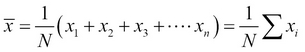
The long-run average value of a random variable is known as the expectation or mean. The sample mean is the corresponding average over the observed data.

In the case of a discrete random variable, the mean is given by:

For example, the mean number of pips turning up on rolling a single fair die is 3.5.

For a continuous random variable with probability density function f(x), the mean is:

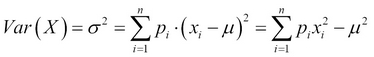
Variance is the expectation of the square of the difference between the random variable and its mean.

In the discrete case, with the mean defined as previously discussed, and with the probability mass function p(x), the variance is:

In the continuous case, it is as follows:

Some continuous distributions do not have a mean or variance.

Standard deviation is a measure of how spread out the data is in relation to its mean value. It is the square root of variance, and unlike variance, it is expressed in the same units as the data. The standard deviation in the case of discrete and continuous random variables are given here:,

The standard deviation of a sample drawn randomly from a larger population is a biased estimate of the population standard deviation. Based on the particular distribution, the correction to this biased estimate can differ. For a Gaussian or normal distribution, the variance is adjusted by a value of .

Per the definition given earlier, the biased estimate s is given by:

In the preceding equation, is the sample mean.

The unbiased estimate, which uses Bessel's correction, is:

In a joint distribution of two random variables, the expectation of the product of the deviations of the random variables from their respective means is called the covariance. Thus, for two random variables X and Y, the equation is as follows:

= E[XY] – μx μy

If the two random variables are independent, then their covariance is zero.

When the covariance is normalized by the product of the standard deviations of the two random variables, we get the correlation coefficient ρ_X,Y, also known as the Pearson product-moment correlation coefficient:

The correlation coefficient can take values between -1 and 1 only. A coefficient of +1 means a perfect increasing linear relationship between the random variables. -1 means a perfect decreasing linear relationship. If the two variables are independent of each other, the Pearson's coefficient is 0.

Discrete probability distribution with parameters n and p. A random variable is a binary variable, with the probability of outcome given by p and 1 – p in a single trial. The probability mass function gives the probability of k successes out of n independent trials.

Parameters: n, k

PMF:

Where:

This is the Binomial coefficient.

Mean: E[X] = np

Variance: Var(X) = np(1 – p)

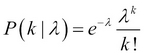
The Poisson distribution gives the probability of the number of occurrences of an event in a given time period or in a given region of space.

Parameter λ, is the average number of occurrences in a given interval. The probability mass function of observing k events in that interval is

PMF:

Mean: E[X] = λ

Variance: Var(X) = λ

The Gaussian distribution, also known as the normal distribution, is a continuous probability distribution. Its probability density function is expressed in terms of the mean and variance as follows:

Mean: µ

Standard deviation: σ

Variance: σ2

The standard normal distribution is the case when the mean is 0 and the standard deviation is 1. The PDF of the standard normal distribution is given as follows:

The central limit theorem says that when you have several independent and identically distributed random variables with a distribution that has a well-defined mean and variance, the average value (or sum) over a large number of these observations is approximately normally distributed, irrespective of the parent distribution. Furthermore, the limiting normal distribution has the same mean as the parent distribution and a variance equal to the underlying variance divided by the sample size.

Given a random sample X1, X2, X3 … Xn with µ = E[Xi] and σ2 = Var(Xi), the sample mean:

is approximately normal

There are several variants of the central limit theorem where independence or the constraint of being identically distributed are relaxed, yet convergence to the normal distribution still follows.

Suppose there is a random variable X, which is a function of multiple observations each with their own distributions. What can be said about the mean and variance of X given the corresponding values for measured quantities that make up X? This is the problem of error propagation.

Say x is the quantity to be determined via observations of variables u, v, and so on:

x = f(u, v, )

Let us assume that:

The uncertainty in x in terms of the variances of u, v, and so on, can be expressed by the variance of x:

From the Taylor expansion of the variance of x, we get the following:

Here, is the covariance.

Similarly, we can determine the propagation error of the mean. Given N measurements with x_i with uncertainties characterized by si, the following can be written:

With:

These equations assume that the covariance is 0.

Suppose si = s – that is, all observations have the same error.

Then, .

Since

Therefore, .