
Performance – Descent
Abstract
The chapter is split into two parts. The first one develops fundamental relationships required to evaluate the characteristics of gliding flight. The second one develops an assortment of methods to predict a number of descent characteristics of an airplane.
Keywords
Equations of motion; free-body; descent; glide; planar; angle-of-descent; rate-of-descent; equilibrium glide speed; sink rate; minimum sink rate; minimum angle-of-descent; best glide; glide distance
Outline
21.1.1 The Content of this Chapter
21.2 Fundamental Relations for the Descent Maneuver
21.2.1 General Two-dimensional Free-body Diagram for an Aircraft
21.2.2 Planar Equations of Motion (Assumes No Rotation about Y-axis)
21.3 General Descent Analysis Methods
21.3.1 General Angle-of-descent
21.3.2 General Rate-of-descent
Derivation of Equation (21-10)
21.3.3 Equilibrium Glide Speed
Derivation of Equation (21-11)
Derivation of Equations (21-12) and (21-13)
21.3.5 Airspeed of Minimum Sink Rate, VBA
Derivation of Equation (21-14)
21.3.6 Minimum Angle-of-descent
Derivation of Equation (21-15)
Derivation of Equation (21-16)
21.1 Introduction
For powered aircraft, the analysis of gliding flight is essential from the standpoint of safety. For unpowered flight, glide performance is what sets one sailplane apart from another. Analysis of descent provides a very important insight into how efficient an airplane is. It can even expose possible handling problems. For instance, a powered airplane with a high glide ratio (L/D ratio) will find this feature very favorable if it experiences engine failure and must rely on this property to get to the nearest emergency airport. However, if the L/D ratio is very high, this will actually make it harder to land as it would have to fly at a very shallow approach path angle to keep the airspeed low. The shallow angle would not only make it more difficult to assess where it will touch-down, but would also tend to make the airplane float once it enters ground effect, compounding the difficulty. Figure 21-1 shows an organizational map displaying the descent among other members of the performance theory.
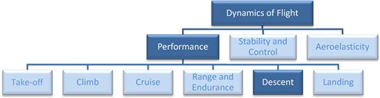
FIGURE 21-1 An organizational map placing performance theory among the disciplines of dynamics of flight, and highlighting the focus of this section: descent performance analysis.
This section will present the formulation of and the solution of the equation of motion for the descent, and present practical, as well as numerical solution methodologies, that can be used both for propeller and jet-powered aircraft. When appropriate, each method will be accompanied by an illustrative example using the sample aircraft. The primary information we want to extract from this analysis is characteristics like minimum rate-of-descent (ROD), best (lowest) angle-of-descent (AOD), the corresponding airspeeds, the AOD for a given power setting, and unpowered glide distance.
In general, the methods presented here are the “industry standard” and mirror those presented by a variety of authors, e.g. Perkins and Hage [1], Torenbeek [2], Nicolai [3], Roskam [4], Hale [5], Anderson [6] and many, many others. Also note that sailplane design and glide analyses methods are detailed in Appendix C4, Design of Sailplanes.
21.2 Fundamental Relations for the Descent Maneuver
In this section, we will derive the equation of motion for the descent maneuver, as well as all fundamental relationships used to evaluate its most important characteristics. First, a general two-dimensional free-body diagram will be presented to allow the formulation to be developed. Only the two-dimensional version of the equation will be determined as this is sufficient for all aspects of aircraft design.
21.2.1 General Two-dimensional Free-body Diagram for an Aircraft
The free body for the descending flight is developed in a similar manner to that for the climbing flight. Figure 21-2 shows a free-body diagram of an airplane moving along a flight path. The x- and z-axes are attached to the center of gravity (CG) of the airplane, just as for the climb and have identical orientation with respect to the datum of the airplane. The angle between the datum and the tangent to the flight path is the angle-of-attack and the force (or thrust) generated by the airplane’s power plant, T, may be at some angle ε with respect to the x-axis. The figure shows that this coordinate system can change its orientation with respect to the horizon depending on the maneuver being performed. Then, the angle between the horizon and the x-axis, the descent angle, is denoted by θ, where these three simple rules apply: If θ > 0, then the aircraft is said to be climbing. If θ = 0 then the aircraft is said to be flying straight and level (cruising). If θ < 0, then the aircraft is said to be descending. This chapter only considers the final rule.
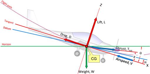
The free-body diagram of Figure 21-2 is balanced in terms of inertia, mechanical, and aerodynamic forces. The lift is the component of the resultant aerodynamic force generated by the aircraft that is perpendicular to the flight path (along its z-axis). The drag is the component of the aerodynamic force that is parallel (along its x-axis). These are balanced by the weight, W, and the corresponding components of T. The presentation of Figure 21-2 can now be used to derive the planar equations of motion for the descent maneuver, which are sufficient to accurately predict the vast majority of descent maneuvers.
21.2.2 Planar Equations of Motion (Assumes No Rotation about Y-axis)
The equations of motion for gliding flight can be derived using the free-body diagram in Figure 21-2:
![]() (21-1)
(21-1)
![]() (21-2)
(21-2)
The equations of motion can be adapted for descending flight by making the following assumptions:
(1) Steady motion implies dV/dt = 0.
(2) The descent angle, θ, is a non-zero quantity.
Equations of motion for a steady unpowered (T = 0) descent:
![]() (21-3)
(21-3)
![]() (21-4)
(21-4)
Equations of motion for a steady powered (T > 0) descent:
![]() (21-5)
(21-5)
![]() (21-6)
(21-6)
![]() (21-7)
(21-7)
AOD is also known as angle-of-glide (AOG) or glide angle.
21.3 General Descent Analysis Methods
21.3.1 General Angle-of-descent
The angle-of-descent is the flight path angle to the horizontal and is computed from:
The right approximations (≈) are valid for low descent angles, θ, and when the CG is not too far forward, as this can put a high load on the stabilizing surface and invalidate the approximation L ≈ W. Many airplanes, in particular sailplanes, have such high glide ratios that landing becomes difficult. For this reason, they are equipped with speed brakes or spoilers, which are panels that deflect from the wing surface and cause flow separation, increasing drag and reducing lift. The same holds for high-speed jets.
21.3.2 General Rate-of-descent
The rate at which an aircraft reduces altitude is given below:
![]() (21-10)
(21-10)
The above expression has units of ft/s or m/s. Generally, the units preferred by pilots are in terms of feet per minute or fpm for general aviation, commercial aviation, and military, but m/s for sailplanes and some nations that use the metric system. To convert Equation (21-10) into units of fpm multiply by 60.
Derivation of Equation (21-10)
Begin by multiplying Equation (21-4) by V, and then rewrite V sin θ using Equation (21-7):
![]()
QED
EXAMPLE 21-1
Plot the rate-of-descent for the Learjet 45XR at S-L, 15,000 ft, and 30,000 ft at a weight of 20,000 lbf (assuming no thrust). Plot the descent rate as a function of true airspeed in knots (KTAS).
Solution
Sample calculation for the sample aircraft gliding at 175 KCAS (LDmax) at S-L and at 20,000 lbf (no thrust). Note that LDmax is calculated in EXAMPLE 19-5.
![]()
At S-L the density is 0.002378 slugs/ft3. Therefore:
![]()
This amounts to 1147 fpm. The rate-of-descent for other airspeeds is plotted in Figure 21-4. Figure 21-5 shows the corresponding glide angle and L/D for the aircraft at S-L. Figure 21-6 shows how important performance characteristics, such as the airspeed for minimum power required and best glide ratio, can be extracted from the rate-of-descent plot.


21.3.3 Equilibrium Glide Speed
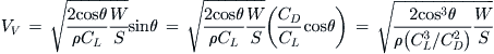
Equilibrium glide speed is the airspeed that must be maintained to achieve a specific glide angle for a specific AOA. One common use is to determine the airspeed required to maintain a specific flight path angle, θ.
![]() (21-11)
(21-11)
The lift coefficient can be determined based on the AOA required for the airspeed using CL = CLo + CLα·α
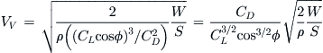
21.3.4 Sink Rate
Sink rate is the rate at which an aircraft loses altitude. This is most commonly expressed in terms of feet per minute or meters per second. If the lift and drag coefficients can be determined for a specific glide condition (e.g. from knowing the AOA), the sink rate can be computed from:

The above expression will return the sink rate in terms of ft/s or m/s. To convert to fpm multiply by 60. If the airplane is turning and the bank angle is given by the bank angle φ, then the sink rate increases and amounts to:
Derivation of Equations (21-12) and (21-13)
Substitute Equation (21-11) into (21-7) to get:
![]() (i)
(i)
Divide Equation (21-4) by (21-3) to get:
![]() (ii)
(ii)
Substitute Equation (ii) into (i) to get:
If we assume cos θ ∼ 1 we get Equation (21-12).
To get Equation (21-13) we refer to Figure 19-26 and see that W = L·cos ϕ = qS·CL·cos ϕ. When level (ϕ = 0°) the same relationship is W = L = qS·CL. This shows that the lift really depends on the product CL·cos ϕ. Therefore, it is more accurate to replace the lift coefficient in the above formulation with the product.
QED
21.3.5 Airspeed of Minimum Sink Rate, VBA
Just like the rate-of-climb, the magnitude of the sink rate varies with airspeed. This implies it has a minimum value that would be of interest to the operator of the vehicle as the kinetic energy of the vertical speed is then also at a minimum and, thus, may have an impact on survivability in an unpowered glide (as impact energy is a function of the square of the speed). It turns out that if the simplified drag model applies, the minimum sink speed can be calculated directly as follows. Note that this expression only holds in air mass that is neither rising nor sinking (see Appendix C4, Design of Sailplanes).
![]() (21-14)
(21-14)
21.3.6 Minimum Angle-of-descent
This angle results in a maximum glide distance from a given altitude and is of great importance to both glider pilots and pilots of powered aircraft.
![]() (21-15)
(21-15)
Note that the drag model yields a θmin which is independent of altitude.
21.3.7 Best Glide Speed, VBG
The best glide speed is the airspeed at which the airplane will achieve maximum range in glide. It is a matter of life and death for the occupants of an aircraft, as is evident from its inclusion in 14 CFR 23.1587(c)(6), Performance Information. A part of pilot training requires this airspeed to be remembered in case of an engine failure. It can be calculated using Equation (21-16) below. Note that this expression only holds in air mass that is neither rising nor sinking (see Appendix C4, Design of Sailplanes).
![]() (21-16)
(21-16)
Derivation of Equation (21-16)
Using Equation (21-11) and the assumption that at the best glide angle cos θ ≈ 1, we get:
![]()
It was demonstrated in the derivation for Equation (19-18) that at LDmax the lift coefficient ![]() . Inserting this into the above expression and manipulating leads to:
. Inserting this into the above expression and manipulating leads to:

QED
EXAMPLE 21-4
Determine the airspeed of minimum angle-of-descent for the sample aircraft flying at 30,000 ft and S-L at a weight of 20,000 lbf.
Solution
At 30,000 ft the density is 0.0008897 slugs/ft3. Therefore:

At S-L the density is 0.002378 slugs/ft3. Therefore:

This amounts to 175 KCAS in both cases.
21.3.8 Glide Distance
For a powered airplane, knowing how far one can glide in case of an emergency is not just a matter of safety, but of survivability. Such information is required information for the operation of GA aircraft by 14 CFR Part 23, §23.1587(d)(10), Performance Information, and must be determined per §23.71, Glide: Single-engine Airplanes (see below) and presented to the operator of the aircraft. This is typically done in the form of a glide chart, which shows clearly how far the airplane will glide for every 1000 ft lost in altitude.
During the design phase, this distance can be calculated from the following expression (which is shown schematically in Figure 21-7). Note that this expression only holds in air mass that is neither rising nor sinking (see Appendix C4, Design of Sailplanes).
![]() (21-17)
(21-17)

Derivation of Equation (21-17)
First we note the following relation between the speed and distance:
![]()
Assuming that θ is small, we can say that![]() . Therefore, using Equation (21-5) we get:
. Therefore, using Equation (21-5) we get:
![]()
Using Equation (21-3) and the assumption that for small angles cos θ ≈ 1, we get:
![]()
QED
EXAMPLE 21-5
Determine the maximum glide distance for the sample aircraft flying at 30,000 ft.
Solution
Using the maximum LD calculated in EXAMPLE 19-7 we get (LDmax = 15.45):
![]()
References
1. Perkins CD, Hage RE. Airplane Performance, Stability, and Control. John Wiley & Sons 1949.
2. Torenbeek E. Synthesis of Subsonic Aircraft Design. 3rd ed. Delft University Press 1986.
3. Nicolai L. Fundamentals of Aircraft Design. 2nd ed. 1984.
4. Roskam J, Lan Chuan-Tau Edward. Airplane Aerodynamics and Performance. DARcorporation 1997.
5. Hale FJ. Aircraft Performance, Selection, and Design. John Wiley & Sons 1984; pp. 137–138.
6. Anderson Jr JD. Aircraft Performance & Design. 1st ed. McGraw-Hill 1998.
7. Raymer D. Aircraft Design: A Conceptual Approach. AIAA Education Series 1996.