Aircraft Drag Analysis
Abstract
A detailed treatise on the estimation of the aerodynamic drag of aircraft is presented. Starting with a discussion about the nature of drag, what contributes to it, how it is modeled, and a number ways drag can be evaluated. Various limitations of methodologies is presented as well. Then, an introduction to the estimation of selected drag coefficients is given, including the basic drag coefficient, CD0, skin friction drag coefficient, CDf, and lift-induced drag coefficient, CDi. A step-by-step evaluation of an actual aircraft (SR22) is given, which is compared to flight test data at the end of the chapter. The next section discusses the drag characteristics of the airplane as a whole and presents methods to estimate the total drag of aircraft. Two drag estimation methods for complete aircraft are presented; the Rapid Drag Estimation Method and the Component Drag Buildup Method. This is followed by the presentation of methods to estimate the drag caused by the addition of necessary imperfections to aircraft, such as antennas, fairings, landing gear, and so on. Additionally, methods to estimate trim drag and cooling drag. Then methods to estimate the drag of existing aircraft from published data such as performance Information are provided. Finally, the drag characteristics of selected aircraft are tabulated. The data is accumulated from various sources and probably represents the largest collection of such data in an aircraft design book to date.
Keywords
Drag; drag model; drag bucket; quadratic drag; minimum drag; profile drag; zero-lift drag; lift-induced drag constant; effective aspect ratio; compressibility; drag count; Oswald's efficiency; span efficiency; additive drag; basic drag; bubble-drag; coefficient of drag; lift-induced drag; lift-induced drag coefficient; lift-to-drag ratio; miscellaneous drag; parasitic drag; pressure drag; skin friction drag; skin friction drag coefficient; component drag buildup; Reynolds number; cutoff Reynolds number; boundary layer; laminar; turbulent; separated; momentum theorem; downwash; upwash; simplified drag model; adjusted drag model; Prandtl-Betz integration; Trefftz-plane; form-factor; interference factor; CRUD; trim drag; cooling drag; drag extraction
Outline
15.1.1 The Content of this Chapter
Total Drag of Subsonic Aircraft
Minimum Drag, Profile Drag, and Zero-Lift Drag, CDmin
15.2.2 Quadratic Drag Modeling
Equivalent Flat Plate Area (EFPA)
Limitations of the Quadratic Drag Model
15.2.3 Approximating the Drag Coefficient at High Lift Coefficients
15.2.4 Non-Quadratic Drag Modeling
15.2.5 Lift-Induced Drag Correction Factors
15.2.6 Graphical Determination of L/Dmax
15.2.7 Comparing the Accuracy of the Simplified and Adjusted Drag Models
15.3 Deconstructing the Drag Model: the Drag Coefficients
15.3.1 Basic Drag Coefficient: CD0
15.3.2 The Skin Friction Drag Coefficient: CDf
Standard Formulation to Estimate Skin Friction Coefficient
15.3.3 Step-by-step: Calculating the Skin Friction Drag Coefficient
Step 1: Determine the Viscosity of Air
Step 2: Determine the Reynolds Number
Step 3: Cutoff Reynolds Number
Step 4: Skin Friction Coefficient for Fully Laminar or Fully Turbulent Boundary Layer
Step 5: Mixed Laminar-Turbulent Flow Skin Friction
Step 6: Mixed Laminar-Turbulent Flow Skin Friction
Step 7: Compute Skin Friction Drag Coefficient
Step 10: Compute the Total Skin Friction Drag Force
Step 1: Determine the Viscosity of Air
Step 2: Determine the Reynold’s Number for Root Airfoil
Step 3: Determine the Reynold’s Number for Tip Airfoil
Step 4: Fictitious Turbulent BL on Root Airfoil – Upper Surface
Step 5: Fictitious Turbulent BL on Root Airfoil – Lower Surface
Step 6: Fictitious Turbulent BL on Tip Airfoil – Upper Surface
Step 7: Fictitious Turbulent BL on Tip Airfoil – Lower Surface
Step 8: Skin Friction for Root Airfoil – Upper Surface
Step 9: Skin Friction for Root Airfoil – Lower Surface
Step 10: Average Skin Friction for Root Airfoil
Step 11: Skin Friction for Tip Airfoil – Upper Surface
Step 12: Skin Friction for Tip Airfoil – Lower Surface
Step 13: Average Skin Friction for Tip Airfoil
Step 14: Average Skin Friction for Complete Wing
Step 16: Skin Friction Drag Coefficient for Complete Wing
Step 17: Skin Friction Drag Force for Complete Wing
Step 18: Skin Friction Coefficient for 100% Laminar Flow
Step 19: Skin Friction Coefficient for 100% Turbulent Flow
15.3.4 The Lift-Induced Drag Coefficient: CDi
Method 1: Lift-Induced Drag from the Momentum Theorem
Method 2: Generic Formulation of the Lift-Induced Drag Coefficient
Derivation of Equation (15-40)
Method 3: Simplified k·CL2 Method
Method 4: Adjusted k·(CL − CLminD)2 Method
Method 5: Lift-Induced Drag Using the Lifting-Line Method
Method 6: Prandtl-Betz Integration in the Trefftz Plane
15.3.5 Total Drag Coefficient: CD
15.3.6 Various Means to Reduce Drag
Reduction of Drag on Wings via Laminar Flow Control (LFC)
Reduction of Drag of Fuselages
Reduction of Drag of the Fuselage/Wing Juncture
15.4 The Drag Characteristics of the Airplane as a Whole
15.4.1 The Effect of Aspect Ratio on a Three-Dimensional Wing
15.4.2 The Effect of Mach Number
15.4.3 The Effect of Yaw Angle β
15.4.4 The Effect of Control Surface Deflection – Trim Drag
15.4.5 The Rapid Drag Estimation Method
15.4.6 The Component Drag Build-Up Method
15.4.7 Component Interference Factors
15.4.8 Form Factors for Wing, HT, VT, Struts, Pylons
15.4.9 Form Factors for a Fuselage and a Smooth Canopy
Fuselage as a Body of Revolution
Form Factors at Subcritical Reynolds Numbers
Form Factors at Supercritical Reynolds Numbers
Form Factor for Nacelle and Smooth External Store
Form Factors for Airship Hulls and Similar Geometries
15.5 Miscellaneous or Additive Drag
Derivation of Equation (15-79)
15.5.1 Cumulative Result of Undesirable Drag (CRUD)
Trim Drag of a Simple Wing-Horizontal Tail Combination
Derivation of Equation (15-80)
Trim Drag of a Wing-Horizontal Tail-Thrustline Combination
Derivation of Equation (15-81)
Derivation of Equation (15-82)
15.5.4 Drag of Simple Wing-Like Surfaces
15.5.5 Drag of Streamlined Struts and Landing Gear Pant Fairings
Drag of Tires with Wheel Fairings
Drag of Fixed Landing Gear Struts with Tires
Drag of Retractable Landing Gear
Increase of CDmin Due to Flaps
15.5.9 Drag Correction for Cockpit Windows
Drag of Conventional Cockpit Windows
Drag of Blunt Ordinary and Blunt Undercut Cockpit Windows
15.5.12 Drag Due to Compressibility Effects
Derivation of Equations (15-106) through (15-107)
15.5.13 Drag of Windmilling and Stopped Propellers
Drag Due to Windmilling Propellers
Drag Due to Stopped Propellers
15.5.15 Drag of Various Geometry
Three-Dimensional Drag of Two-Dimensional Cross-Sections of Given Length
Drag of Three-Dimensional Objects
15.5.17 Drag of Various External Sources
Drag of Sanded Walkway on Wing
Drag of Gun Ports in the Nose of an Airplane
Drag of Streamlined External Fuel Tanks
15.5.18 Corrections of the Lift-Induced Drag
Correction of Lift-Induced Drag in Ground Effect
15.6 Special Topics Involving Drag
15.6.1 Step-by-step: Extracting Drag from L/Dmax
Step 1: Gather Information from the Vehicle’s POH
Step 2: Convert VLDmax into Units of ft/s
Step 3: Calculate the Best Glide Lift Coefficient
Step 4: Calculate Span Efficiency
Derivation of Equation (15-123)
15.6.2 Step-by-step: Extracting Drag from a Flight Polar Using the Quadratic Spline Method
Step 1: Select Representative Points from the Flight Polar
Step 3: Fill in the Conversion Matrix and Invert
Step 4: Determine the Coefficients to the Quadratic Spline
Step 5: Extract Aerodynamic Properties
Derivation of Equations (15-124) through (15-127)
15.6.3 Step-by-step: Extracting Drag Coefficient for a Piston-Powered Propeller Aircraft
Method 1: Extraction CDmin Using Cruise Performance
Derivation of Equation (15-128)
Method 2: Extracting CDmin Using Climb Performance
Derivation of Equation (15-129)
15.6.4 Computer code 15-1: Extracting Drag Coefficient from Published Data for Piston Aircraft
15.6.5 Step-by-step: Extracting Drag Coefficient for a Jet Aircraft
Derivation of Equation (15-130)
Derivation of Equation (15-131)
15.6.6 Determining Drag Characteristics from Wind Tunnel Data
Derivation of Equations (15-132) through (15-134)
15.7 Additional Information – Drag of Selected Aircraft
15.7.1 General Range of Subsonic Minimum Drag Coefficients
15.1 Introduction
Few tasks in aircraft design are as daunting as the estimation of drag. Not only does drag put a lid on what is possible, it can also convert what seems like a promising idea into a terrible one. As far as aircraft design is concerned, the primary objective is usually to minimize drag. However, there is much more to drag than meets the eye. In spite of a desire to keep it as low as possible, ideally we want to control it. Sometimes it is preferable to temporarily increase it and even to shift it around. During climb and cruise, the drag should be kept as low as possible. However, during approach to landing, higher drag helps slow down the airplane and makes it easier to control it during landing. Sailplane pilots can attest to how hard it would be to land a sailplane if such aircraft did not feature spoilers to help them avoid overshooting the runway. For some aircraft, including many sailplanes, it is possible to shift the drag polar around using a cruise flap. This permits the pilot to move the maximum glide ratio to a higher airspeed, which is desirable if one wants to glide it as far as possible. The bottom line is that a good understanding of what the drag consists of, what affects it and what does not, is imperative to the designer. The purpose of this section is to provide the aircraft designer with methods to estimate drag and details of its causes and prevention.
Many areas of the aircraft design process rely on accurate drag estimation. This includes performance analysis, engine selection, and requirements for fuel capacity, to name a few. The subject must be approached with great respect and caution. Drag is extremely hard to predict accurately, but instead easy to over- and underestimate. This does not mean that the calculations themselves are exceedingly difficult, but rather that the sources that contribute to the drag may be hard to identify. The accuracy of the calculations is vitally important as an underestimation will result in an airplane that performs far worse than predicted, risking a costly “drag-cleanup” effort if not the cancellation of an otherwise viable program. By the same token, an overestimation by an overly conservative approach may render the design so bad on paper the project might be cancelled before it even begins.
The aspiring designer should not think that the problem of drag estimation can be solved by simply modeling the aircraft using a Navier-Stokes computational fluid dynamics (NS CFD) solver. This view is often heard uttered by students of aerospace engineering who have yet to be humbled by Mother Nature by comparing predictions to actual wind tunnel or flight testing. While CFD is both a very promising and exciting scientific advance, the technology is not yet robust enough to allow a novice user to estimate drag reliably.1 In 2001, the AIAA2 conducted the first of four workshops on drag estimation using NS CFD methods. A clean Airbus-style passenger transport aircraft, consisting of a fuselage and wing only, was modeled by 18 participants using 14 different NS solvers. Then the analysis results were compared to the wind tunnel data, which was not made available to the participants until after the analysis results had been submitted. In short, the lift and drag predictions were all over the map. Some models predicted lift and drag close to the wind tunnel data, while for others the deviation of the drag polar ranged from approximately 50% to 200% of the wind tunnel value [1,2]. These predictions were performed by scientists who were experts in the use of these codes. If they have a hard time performing such predictions, the novice analyst should take caution. The drag analyst is in many ways between a rock and a hard place – a dreaded place shared by the weights engineer.
In this section, classical methods will be used to estimate the magnitude of the drag. In spite of what is stated above, these methods (like the NS methods) can yield good predictions as long as they are applied with caution. As stated in Section 8.1, drag, D, is defined as the component of the resultant force, R, which is parallel to the trajectory of motion (see Figure 15-1). The force of drag differs from the force of lift in that its constituent contributors are both pressure difference and friction. Like lift, drag is a component of the resultant force that results from the pressure differential over a body. Friction, however, is a force that acts parallel to the airspeed, which explains why it contributes only to the drag and not the lift. The purpose of performing a drag analysis is to estimate the magnitude of this force and understand how the geometry, as well as attitude of the aircraft and flight condition, affects its magnitude.
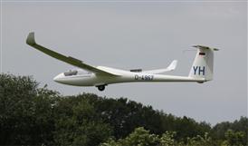
FIGURE 15-1 No aircraft generate as little drag as the modern sailplane. A Rolladen-Schneider LS4 sailplane, moments before touchdown with spoilers deployed. (Photo by Phil Rademacher)
Classical drag estimation methods attempt to predict drag based on geometry and flow properties. Any useful drag estimation method must account for:
Non-dimensional coefficients are essential when working with aerodynamic forces and moments. With respect to the drag of aircraft, the coefficient form that represents the total drag is referred to as the drag model. A drag model is a mathematical expression that when multiplied by dynamic pressure and a reference area will yield the drag force acting on the aircraft. It can be used in a number of important ways, ranging from plotting the drag polar (a graph in which the drag coefficient is plotted as a function of the lift coefficient) to evaluating important performance characteristics such as the lift coefficient to maintain in flight to achieve the longest glide distance or fly farthest.
Generally, the total drag of an airplane is broken into two classes attributed to flow separation (pressure drag) and skin friction (skin friction drag). Thus, the drag consists of the following contributions:
(1) Basic pressure drag is caused by the pressure differential formed by the airplane that acts parallel to the tangent to the flight path.
(2) Skin friction drag is caused by the “rubbing” of molecules along the surfaces of the airplane.
(3) Lift-induced drag is caused by the circulation around the wing, which tilts the lift vector backwards, creating a force component that adds to the total drag.
(4) Wave drag is caused by the rise in pressure around a body due to the formation of a normal shock wave on the airplane. This effect begins at high subsonic Mach numbers.
(5) Miscellaneous drag is caused by a number of “small” contributions that are often easily overlooked, such as small inlets and outlets, access panels, fuel caps, to name a few.
In this section we will present methods to determine all of these types of drag, although wave drag will be treated with far less detail than the others since it is a high subsonic phenomenon. To do this, a number of drag modeling methods will be presented and the effects of various flow phenomena will be explained. Then, we will present a method to estimate the skin friction on lifting surfaces that are assumed smooth and continuous. The method assumes a minimum level of flow separation and assumes a mixed boundary layer. A mixed boundary layer is one in which a laminar boundary layer is allowed to transition into a turbulent one. This method is superior to methods that consider the boundary layer to be either laminar or turbulent, as it treats the flow more realistically than either of these. Then, we will introduce the effect that changing the AOA or AOY has on the drag, in terms of both increased level of separated flow and increase in drag due to lift. Then, special methods will be introduced that allow the total drag to be estimated for an airplane as a whole. This will be followed by a number of specialized methods to estimate the drag of parts of the airplane, such as drag due to engine cooling requirements. Finally, methods will be presented that allow the drag of an existing aircraft to be extracted using specific, publically available data.
Today, the state-of-the-art in low drag aircraft is the modern sailplane (see Figure 15-1). Natural laminar flow (NLF) airfoils, segmented tapered wing planform, tadpole fuselage, sealed control surfaces, carefully tailored wing root fairings, T-tail, and disciplined attention to any detail that reduces drag, combine to make some sailplanes capable of achieving glide ratios in excess of 1:50. No other aircraft are capable of that – flying wing or not. The aircraft designer interested in developing a low-drag aircraft should pay special attention to such aircraft. There is a lot that can be learned.
15.1.1 The Content of this Chapter
• Section 15.2 discusses the nature of drag, what contributes to it, how it is modeled, and a number ways drag can be evaluated. The section also discusses various limitations to how it is evaluated.
• Section 15.3 discusses the drag coefficient, including the basic drag coefficient, CD0, skin friction drag coefficient, CDf, and lift-induced drag coefficient, CDi.
• Section 15.4 discusses the drag characteristics of the airplane as a whole and presents methods to estimate the total drag of aircraft.
• Section 15.5 presents methods to estimate the drag caused by the addition of necessary imperfections to aircraft, such as antennas, fairings, landing gear, and so on. Additionally, methods to estimate trim drag and cooling drag are presented.
• Section 15.6 presents methods to estimate the drag of existing aircraft, using data such as published performance data.
• Section 15.7 presents the drag characteristics of selected aircraft, accumulated from various sources.
15.2 The Drag Model
A drag model is a mathematical expression of the drag coefficient that describes how the drag of the body changes as a function of its orientation in the flow field. The determination of this model is a challenging task, although good analytical approximations are possible at lower AOAs, as we will show shortly. The difficulty in devising good drag models at higher AOAs stems from the fact that they are highly dependent on the size of the flow separation regions and these are very difficult to predict accurately. And as stated in the introduction to this section, even state-of-the-art formulations of fluid flow implemented in Navier-Stokes solvers have a hard time doing this well. The most reliable methods remain wind tunnel or flight testing.
Since our purpose here is to build tools to help us predict the drag of the airplane before a wind tunnel testing is conducted, let alone flight testing, we more than anything else seek a realistic model of the drag. First we note that a realistic mathematical presentation for drag, D, can be written as shown below:
![]() (15-1)
(15-1)
where geometry refers to reference and wetted area.
The standard way to estimate the drag is to represent the dependency on airspeed and density through the dynamic pressure, ![]() , the geometry using a reference area, Sref, and the remaining dependencies are lumped into the drag coefficient, denoted by CD. Thus, we compute the drag, D, using the expression:
, the geometry using a reference area, Sref, and the remaining dependencies are lumped into the drag coefficient, denoted by CD. Thus, we compute the drag, D, using the expression:
![]() (15-2)
(15-2)
where
The drag coefficient in Equation (15-2) is the drag model.
15.2.1 Basic Drag Modeling
Basic drag modeling is the mathematical combination of all sources of drag for a vehicle, such that the effect of changing its orientation with respect to its path of motion and fluid velocity is realistically replicated. This modeling culminates in the determination of the total drag coefficient, CD.
As stated in the introduction, the total drag coefficient comprises the effect of basic pressure drag, skin friction drag, lift-induced drag, wave drag, and contributions from other sources, commonly referred to as miscellaneous drag. Typically, basic pressure drag, skin friction drag, and miscellaneous drag are lumped together and are represented using a single number, called the minimum drag, as is done in the so-called quadratic drag modeling. This is accomplished using a special method called the component drag build-up method, presented later in the chapter.
In short, the method estimates the total drag by determining the skin friction drag of a particular component (e.g. the wing or the HT). Then the basic pressure drag is accounted for using a booster factor called a form factor, presented in detail later in this chapter. Thus, the designer estimates the skin friction coefficient for the surface and then multiplies it by the form factor, yielding a number that, as stated earlier, combines the effect of friction and pressure. Additionally, it is necessary to account for the numerous protrusions and discontinuities in the generally smooth surfaces of the aircraft, as it results in greater than expected pressure drag. This drag is called miscellaneous drag.
As the AOA or AOY changes, the contribution of the pressure drag terms increases, adding non-linearity to the formulation that is usually not accounted for in the modeling. It is acceptable to omit this effect for low values of AOA and AOY. However, once a certain orientation is reached, the pressure drag grows to a magnitude so large that it can no longer be ignored. Then, standard drag models are no longer acceptable unless a means to capture this effect is included. A method to account for this high AOA effect is presented in Section 15.2.3 of this chapter.
Total Drag of Subsonic Aircraft
In an ideal world, the total drag coefficient can be considered as the combination of a number of constituent components:
![]() (15-3)
(15-3)
where
CDo = basic drag coefficient (pressure drag)
CDf = skin friction drag coefficient
Each component depends on the aircraft’s geometry, as well as its orientation and airspeed. For low subsonic aircraft the norm is to omit wave drag, which simplifies Equation (15-3) as follows:
![]() (15-4)
(15-4)
Minimum Drag, Profile Drag, and Zero-Lift Drag, CDmin
As stated above, CDo, CDf, and CDmisc are lumped in a single number that from now on will be referred to as CDmin or minimum drag coefficient. This is also referred to as a profile drag or parasitic drag or zero-lift drag, although this book will only use the term minimum drag. The minimum drag coefficient represents the lowest drag the vehicle will generate. The advantage of combining the CDo, CDf, and CDmisc in this fashion is that it allows for a simple evaluation of the total drag coefficient. However, the convenience hides the contribution of the wetted area on the overall airplane drag.
15.2.2 Quadratic Drag Modeling
A standard way to present the drag coefficient is to relate it to the lift coefficient using a quadratic polynomial in accordance with the derivation presented in Section 15.3.4, The lift-induced drag coefficient: CDi. The method can provide an accurate prediction over a range of lift coefficients, although the accuracy drops rapidly at the extremes of the drag polar. A standard “simplified” quadratic presentation for the drag coefficient is:
![]() (15-5)
(15-5)
where
A far more “realistic” presentation for the drag coefficient is the adjusted drag model, represented graphically in Figure 15-2.
![]() (15-6)
(15-6)
where CL minD = the lift coefficient where drag becomes a minimum.
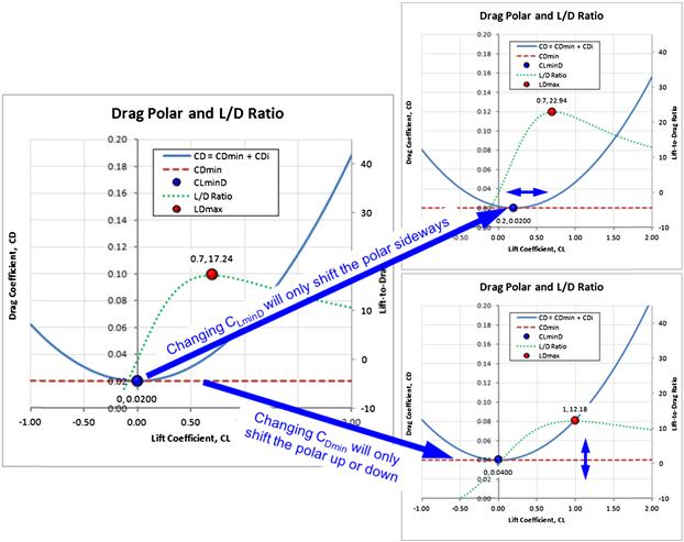
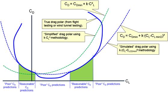
Two important properties of the adjusted drag polar are shown in Figure 15-2. Changing the CLminD will only shift the polar sideways. If CLminD < 0 then the curve will be shifted left, but if CLminD > 0 it will be shifted right. Similarly, changing the value of the CDmin will shift the polar up or down. Of course CDmin is always larger than zero, whereas CLminD can range from a negative to a positive number depending on the camber of the airfoil, or, in the case of a complete aircraft, the effective camber of the entire geometry.
Lift-Induced Drag Constant, k
This is the constant whose product with the lift coefficient squared yields the lift-induced drag. It is given by:
![]() (15-7)
(15-7)
Effective Aspect Ratio, ARe
The product AR·e is often referred to as the effective aspect ratio, denoted by ARe. In this respect, the Oswald (or spanwise) efficiency can be considered a factor that renders the AR less effective than the geometric value would indicate. The designer can consider planform and other geometric modifications, such as endplates or winglets, to increase the effective AR, but should be aware that such modifications increase the skin friction drag. Note that for a clean wing, if ARe → ∞ then k → 0 and therefore CD → Cd, i.e. the drag coefficient effectively becomes that of the airfoil.
CD Dependency on α and β
Sometimes, CDo and CDf are treated as if they are constant with respect to α and β. This is not true in real airflow and they are treated this way for convenience. Changes in α and β will move the laminar to turbulent flow transition line and reshape flow separation regions. This changes the pressure drag, modifying the basic drag coefficient.
Consequently, changing α and β will change CDmin, but this change is not to be confused with the simultaneous change in the induced drag, CDi, whose magnitude is related to the lift coefficient, CL. If the airspeed is mostly unchanged, the change in CDmin can considered solely due to a change in the size of flow separation areas over the airplane, distinguishing it from pressure changes that directly modify lift generation and, thus, affect CDi.
Compressibility Effects
The effect of compressibility is accounted for by modifying CDmin at high subsonic airspeeds using a special correction factor (see Section 15.5.12, Drag due to compressibility effects). In addition to this effect, CDf should also be corrected using methods such as the Frankl-Voishel one of Section 8.3.6, Compressibility modeling. This will also modify CDmin.
Drag Counts
A “drag count” is the drag coefficient multiplied by a factor of 10000. For instance, 250 drag counts is equivalent to a CD = 0.0250; 363 drag counts is equivalent to a CD = 0.0363, and so on.
Equivalent Flat Plate Area (EFPA)
The equivalent flat plate area (denoted by f) is a value that is helpful when comparing the relative drag of different aircraft. It is simply the product of the minimum drag coefficient and the reference area, as shown below. Alternatively, this is nothing but the minimum drag force at the given airspeed, Dmin, divided by the dynamic pressure, q:
![]() (15-8)
(15-8)
The concept assumes the drag of the airplane is equivalent to that of a fictitious plate that has a drag coefficient CD = 1.0. Thus, if the flat plate area of an airplane is 10 ft2, it means its drag amounts to that of a flat plate of the same area moving normal to the flight path. The concept is bogus in many respects. For instance, it disregards the effect of Reynolds and Mach numbers (the CD of a flat plate at Re around 105 is actually closer to 1.17; e.g. see Figure 15-66), and no notion is given as to the true geometry of this “plate” (i.e. is it rectangular or circular or any other shape?). In spite of these shortcomings, as stated earlier, it is helpful mostly for comparison purposes. Table 15-18 lists the EFPA for a number of different aircraft.
Limitations of the Quadratic Drag Model
The drag of some aircraft cannot be accurately represented with the quadratic drag model. A sailplane is an example of such an aircraft. Super-clean aerodynamics and natural laminar flow (NLF) result in a drag bucket for the entire vehicle. Consequently, the quadratic approximation will give erroneous values of the max lift-to-drag ratio and where it occurs. The quadratic model works well for airplanes that do not have a noticeable drag bucket, except at very high or very low lift coefficients (see Figure 15-3). The designer must be aware of this limitation as it leads to erroneous prediction of best endurance and range airspeeds, in particular of airplanes with very low wing loading (LSA aircraft). See Section 15.2.7, Comparing the accuracy of the simplified and adjusted drag models for a comparison of the quadratic drag models to actual wind tunnel data for further understanding of the limitation of these models. Also see Section 15.2.3, Approximating the drag coefficient at high lift coefficients for a method to help approximating the deviation at higher lift coefficients.

Drag of Airfoils and Wings
Figure 15-4 shows the effect of taking the leap from a two-dimensional airfoil to a three-dimensional wing (featuring the airfoil). The two-dimensional drag polar for the airfoil consists of (1) a constant drag component (Cdmin), which is attributed to skin friction, and (2) a parasitic increase caused by increase in pressure drag due to the flow separation on the airfoil, which increases with the AOA. Typically this depends on the lift coefficient squared as shown in Equations (15-5) and (15-6). Introducing this airfoil to a finite-aspect-ratio wing will increase the drag further due to the three-dimensional effects: the lift-induced drag. In this case, we express the drag as follows:
![]() (15-9)
(15-9)
where
CL minD = lift coefficient where drag becomes a minimum
CD = total three-dimensional drag coefficient
![]() lift-induced drag constant (see Section 15.3.4)
lift-induced drag constant (see Section 15.3.4)
m = coefficient indicating the parasitic drag increase of the airfoil, obtained from its drag polar
e = span efficiency (note difference from Equations (15-5) and (15-6)
Note that this can be expanded to give the following expression:
![]() (15-10)
(15-10)
The expansion shows that the minimum drag increases by a small factor, ![]() , which shifts the polar a small amount vertically. This is shown in Figure 15-4.
, which shifts the polar a small amount vertically. This is shown in Figure 15-4.

15.2.3 Approximating the Drag Coefficient at High Lift Coefficients
Figure 15-3 reveals a critical problem in all drag modeling; at higher CLs, the drag model deviates drastically from the actual drag and underpredicts it severely. The deviation is caused by a rapid growth of flow separation with AOA and the second-order approximation cannot keep up with the resulting increase in drag. This is a serious problem when estimating aircraft performance at low airspeeds. Therefore, important airspeeds, such as best angle of climb, minimum rate of descent, and others, are shifted to lower airspeeds than observed in practice. This section addresses this shortcoming and develops a method to approximate the rapid rise in drag at higher lift coefficients.
Consider the hypothetical wind tunnel test data in Figure 15-5. Simply stated, the data presented cannot be approximated satisfactorily using a quadratic polynomial. Neither the simplified nor the adjusted drag models will provide acceptable drag prediction at high (or low) lift coefficients. For this reason, only the data points at lower lift coefficients are used to create a curve-fit (or a trend curve). For the wind tunnel data shown in Figure 15-5, assume that a standard adjusted drag model has been determined and, as shown, it agrees well with the measured drag at lower lift coefficients. This model is given by Equation (15-6), reproduced below for convenience:
![]() (15-6)
(15-6)
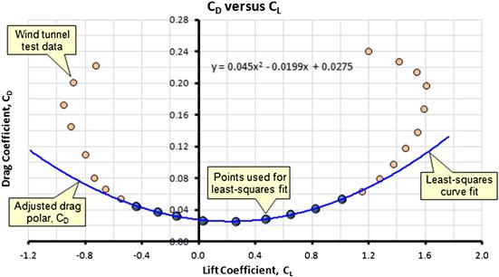
FIGURE 15-5 A hypothetical drag polar for an aircraft, showing the inaccuracy of the quadratic drag model at higher (or lower) lift coefficient.
As is very evident from the graph, the test data begins to deviate sharply from the curve starting at CL = 1.15 (and CL = −0.45). Of course we are primarily interested in the positive lift coefficient, as this is needed for low-speed performance predictions. In order to work around this predicament, the author has used the following methodology in the past with very satisfactory results. In this method, once the CL exceeds a certain value, which here will be called CLm, a quadratic (or cubic) spline is created to simply replace the values of the adjusted drag model.
The method presented here effectively defines a new quadratic polynomial and splices it to the adjusted drag model at CLm. Other splines are certainly possible; however, the advantage of the quadratic spline is the simplicity of its determination and the acceptable accuracy it provides. The method allows the spline to blend smoothly with the underlying adjusted drag model. The first step is to define a modified drag coefficient to be used for CL > CLm. It can be represented by:
![]() (15-11)
(15-11)
Ultimately, the task is to define the constants A, B, and C so CDmod can be evaluated. To do this, two conditions have to be satisfied at CLm:
A third condition is needed to finalize the determination of the coefficients; it is that the value of CDmod at CLmax must match that of the wind tunnel data. That aside, the function for CDmod has three constants (A, B, C) so three equations are required to determine them. One of the equations requires the derivative of both CD and CDmod to be determined. These are presented below:
Now the three equations that allow the constants A, B, and C to be determined can be written as follows:
Rearranging this in a matrix form yields the following expression that allows A, B, and C to be determined using any matrix method, Cramer’s rule or matrix inversion methods:
 (15-12)
Then, once A, B, and C have been determined the drag model is further refined as follows:
![]()
This model has been implemented in Figure 15-6. The improvements in the capability of the drag model are demonstrated by how the quadratic spline, represented by CDmod, smoothly follows the wind tunnel data starting at CLm. Note that although wind tunnel data is assumed here, the same approach can also be used for analytical estimation of the drag coefficient. For such work, it is reasonable to select CLm as the value ½(CLminD + CLmax) as a first guess.
EXAMPLE 15-1
Consider the hypothetical wind tunnel data shown in Figure 15-6. Assume it represents an airplane whose AR = 9. Further assume the least-squares quadratic curve-fit for the data points has been determined and is given by:
![]()
Determine the coefficients for a quadratic spline, assuming a CLm = 1.15, and write the complete drag coefficient using the spline. Note the resulting graph is shown in Figure 15-7.
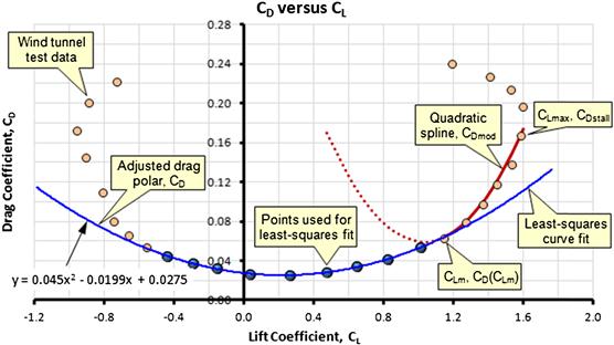
FIGURE 15-6 The same hypothetical drag polar, showing the improvement in prediction accuracy at higher lift coefficients by the introduction of the quadratic spline, CDmod.
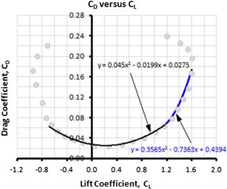
FIGURE 15-7 The modified drag model fits the wind tunnel data better than a regular quadratic model.
Solution
First, using the above drag polar, extract CDmin, CLminD, and the Oswald span efficiency (e) using the conversion method of Section 15.6.6, Determining drag characteristics from wind tunnel data. In particular, see Equations (15-132), (15-133), and (15-134). The section presents an example as well, so only the results based on the above polynomial will be presented.
![]()
![]()
![]()
Using e, we find the k = 1/(π·AR·e) = 0.045. Using this data, the matrix of Equation (15-12) becomes:

From which we find that A = 0.3565, B = −0.7363, and C = 0.4394. The resulting CD can thus be represented by:
![]()
15.2.4 Non-Quadratic Drag Modeling
Figure 15-3 shows that the quadratic model may indeed work well for a specific range of lift coefficients provided a proper value of span efficiency, e, is selected. However, this is not always the case. There are two other instances where the quadratic modeling is simply inadequate and must be abandoned. The first one involves very high or very low lift coefficients, when large areas of separated flow have formed on the airplane. This was treated in the previous section. The second one pertains to aerodynamically clean aircraft, such as sailplanes, for which a well-defined drag bucket exists and is not masked by the drag of other sources that cannot be described by the quadratic formulation. These problematic regions are easily visible in Figure 15-8. In this case, the performance formulation in Chapters 13 through 18 must be revised to account for those cases.
Generally, the presence of the drag bucket will prevent the use of polynomials, as these are not capable of following the sharp change in curvature of the drag polar. Even polynomials of very high order (16+) will not be adequate, as they tend to oscillate inside the prediction region. There are primarily two other methods that can be used to represent such drag polars; a spline (e.g. B-spline) or a lookup table.
15.2.5 Lift-Induced Drag Correction Factors
The estimation of drag due to lift of a three-dimensional wing requires a correction of the two-dimensional airfoil data. This is expressed in Equations (15-5) and (15-6) using the factor e with the induced drag components. There are generally two kinds of such correction factors (although some use them interchangeably):
Oswald Efficiency
The Oswald efficiency is used when calculating the induced drag coefficient for a wing or an aircraft whose dependence on the lift coefficient can be represented with the simplified or adjusted drag models. This is the factor e in Equations (15-5) and (15-6).
Span Efficiency
The span efficiency is used when calculating the drag increase purely based on the three-dimensional increase as shown in Figure 15-4. It does not account for the parasitic drag increase as shown in the figure, but only the three-dimensional effects. This is the factor e in Equation (15-9).
Lift-induced drag is presented in more detail in Section 15.3.4, The lift-induced drag coefficient: CDi.
15.2.6 Graphical Determination of L/Dmax
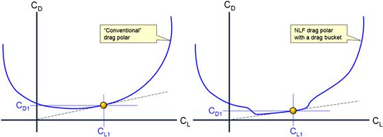
In the absence of knowing the exact numbers of a particular drag polar, it is possible to determine the maximum lift-to-drag ratio, as well as the lift coefficient at which it occurs, graphically. This is shown in Figure 15-9 for a “conventional” drag polar and one for a NLF airfoil (or aircraft) featuring a drag bucket. This is done by fairing a line from the origin so it becomes a tangent to the polar. The reason why this yields L/Dmax can be visualized by recognizing that the tangent aligns with the smallest value of CD at the greatest value of CL.
15.2.7 Comparing the Accuracy of the Simplified and Adjusted Drag Models
The accuracy of the simplified and adjusted drag models can best be illustrated by comparing them to wind tunnel data. One such comparison is shown in Figure 15-10, which compares experimental wind tunnel test results to the simplified and adjusted drag models using Equations (15-5) and (15-6), respectively. Of course it should be emphasized that ordinarily one would not use these models with the drag polar of a two-dimensional airfoil, but a three-dimensional wing. However, this particular illustration can be justified based on Equation (15-9) as the purpose is to show the importance of the term ClminD, here using the lower-case subscript for forces.
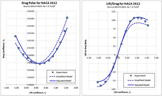
The comparison was implemented using wind tunnel data for the NACA 2412 airfoil obtained from NACA R-824. This airfoil is used on a number of Cessna aircraft designs, for instance the Model 150, 152, 172, and 182, to name a few. First, the drag polar was digitized and the smallest experimental value of the Cd selected for use as the Cdmin for each drag model. Second, the corresponding ClminD to use with the adjusted model was determined by trial and error. Third, the induced drag contribution was calculated using the expressions ![]() for the simplified model and
for the simplified model and ![]() for the adjusted model and added to the Cdmin. Then, k was varied to get the best fit of each model (note both models used the same k). The value of k that best fit the experiment was found to be k ≈ 62.3 The graphs show that the adjusted drag model provides a substantially better fit than the simplified one, in particular for the positive values of the Cl. Another lesson to be learned is the dire consequences of estimating range for an aircraft using the simplified model. Since range depends so explicitly on the CL/CD (see Section 20.2, Range Analysis) a prediction using the simplified drag model would yield a range much less than the adjusted (or experiment) indicates. The opposite can also happen, i.e. the CL/CD using the simplified model is sometimes higher than experiment. The important lesson is that the adjusted model better matches experiment; the simplified does not and should be avoided.
for the adjusted model and added to the Cdmin. Then, k was varied to get the best fit of each model (note both models used the same k). The value of k that best fit the experiment was found to be k ≈ 62.3 The graphs show that the adjusted drag model provides a substantially better fit than the simplified one, in particular for the positive values of the Cl. Another lesson to be learned is the dire consequences of estimating range for an aircraft using the simplified model. Since range depends so explicitly on the CL/CD (see Section 20.2, Range Analysis) a prediction using the simplified drag model would yield a range much less than the adjusted (or experiment) indicates. The opposite can also happen, i.e. the CL/CD using the simplified model is sometimes higher than experiment. The important lesson is that the adjusted model better matches experiment; the simplified does not and should be avoided.
15.3 Deconstructing the Drag Model: the Drag Coefficients
In this section we will discuss the constituent parts of the drag model; the basic, skin friction, and lift-induced drag coefficients.
15.3.1 Basic Drag Coefficient: CD0
The basic drag is a pressure drag force caused by resultant pressure distribution over the surface of body. It can be thought of as the component of the pressure force parallel to the tangent to the flight path. For instance, consider a cylinder in a moving fluid. Its drag consists of the friction between its surface and the moving fluid, and the difference in pressure along its surface. The latter will be the focus in this section. The force is the product of the pressure acting on a cross-sectional area of the body, normal to the flight path.
![]() (15-13)
(15-13)
where
A simple interpretation of the basic drag is shown in Figure 15-11, which shows a sphere moving through a fluid forming a high-pressure region in front of it (left) and a low-pressure region behind it as the turbulent wake. The pressure differential across its cross-sectional area yields a drag force. Equation (15-13) can be rewritten for simple geometry and uniform pressure distributions as follows:
![]() (15-14)
(15-14)

For other geometries, this force increases at high (and low) AOAs as the separation regions grow. If the basic drag force is known, the basic drag coefficient it is defined as follows:
![]() (15-15)
(15-15)
where
D0 = basic drag force in lbf (UK system) or N (SI system)
ρ = air density, typically in slugs/ft3 or kg/m3
V∞ = far-field airspeed, typically in ft/s or m/s
The basic drag coefficient is typically a function of:
![]() (15-16)
(15-16)
where
Ultimately, the basic drag force can be thought of as the increase in the skin friction forces due to the applied form factor (FF), i.e. the difference (FF − 1). However, and as will be seen later, this distinction is better suited for explanation than utility, as it is far more practical to combine the two (i.e. the skin friction and pressure drag contributions). This is due to the complex interaction between the two and our desire to maintain a level of simplicity in our analyses.
15.3.2 The Skin Friction Drag Coefficient: CDf
The skin friction drag coefficient is defined as follows:
![]() (15-17)
(15-17)
where
Df = skin friction drag force in lbf (UK system) or N (SI system)
ρ = air density, typically in slugs/ft3 or kg/m3
V∞ = far-field airspeed, typically in ft/s or m/s
Swet = wetted area, typically in ft2 or m2
Note the difference between the two coefficients Cf and CDf.
Skin friction is caused by a fluid’s viscosity as it flows over a surface. Its magnitude depends on the viscosity of the fluid and the wetted (or total) surface area in contact with it, as well as the surface roughness. The analysis of skin friction drag is complicated by the process of transition, when the laminar boundary layer becomes turbulent. Consequently, this is called a mixed boundary layer. A realistic drag analysis always assumes a mixed boundary layer.
An airfoil that can sustain laminar flow as far aft as 50% of the chord, naturally and on its own merit, is referred to as a natural laminar flow airfoil (NLF). Such airfoils generate substantially less drag than airfoils not capable of this.
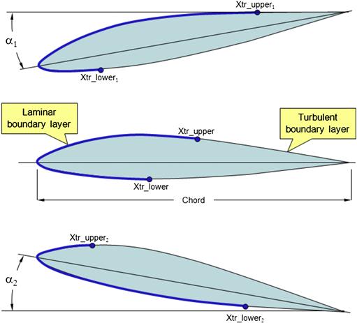
Figure 15-12 shows an airfoil immersed in airflow, on which the laminar boundary layer extends from the leading edge to a point on the upper surface denoted by Xtr_upper and Xtr_lower on the lower surface. At those points, enough instability has developed in the boundary layer to change the laminar profile into a thicker turbulent one. This is the consequence of dynamic flow forces becoming larger than the viscous forces (see Figure 15-13) and tends to occur once the Reynolds number (Re), as measured from the leading edge (LE) along the surface, approaches and exceeds 1 million (on a flat and smooth plate) [3, pp. 2–8]. As the speed of the fluid increases (increasing the Re) the transition points will move farther and farther forward, although they will never fully get to the LE. Therefore, if smooth, the LE will always develop some laminar BL.

The stability of the boundary layer also depends on the geometry and quality of the surface over which the fluid flows. The presence of rivet-heads, uneven plate joints, insects, and even paint chips can destabilize the laminar boundary layer and initiate an early transition (see Section 8.3.13, The effect of leading edge roughness and surface smoothness). Figure 15-14 depicts how the boundary layer changes with AOA. At a low AOA, the transition location on the upper surface is close to the trailing edge, stabilized by the high pressure along the upper surface. At a high AOA, the transition point moves forward, leaving less area covered by the laminar boundary layer. However, and this is important to keep in mind, the laminar boundary layer is more stable on the lower surface because of a net reduction in airspeed.
The boundary layer develops on the surfaces of a “streamlined” three-dimensional shape in a similar fashion as it does on a flat plate and is affected by all the same shortcomings. The velocity distribution in a laminar or turbulent boundary is also similar between the two, albeit being affected by the pressure distribution of the three-dimensional geometry [3, pp. 2–6].
Figure 15-15 shows an important property of flow around an airfoil that ensures the maintenance of the laminar boundary layer (assuming the surface quality is smooth). This property is an extensive region of a favorable pressure gradient. The figure shows the pressure distribution along the chord of two airfoils of 12% thickness-to-chord ratio; a NACA 64-012A and NACA 0012. Both airfoils are at an AOA of 0°. The pressure distribution of the former is represented by the solid line and the latter by the dashed line. The figure also shows that the pressure along the surfaces of the NACA 64-012A airfoil is dropping, starting behind the leading edge until 40% of the chord. The pressure on the NACA 0012 airfoil drops sharply until 12% of the chord. The laminar flow of the 64-012A extends to 55% of the chord, versus 50% of the 0012, and, consequently, it generates slightly less drag. In practice, the transition point of the NACA 0012 would be expected to be farther forward than that.

FIGURE 15-15 Difference in the chordwise pressure distribution of “laminar” and “turbulent” BL airfoils.
One way to achieve such an extensive laminar boundary layer is to place the maximum thickness of the airfoil as far aft as possible. The goal is to allow the fluid to accelerate as far aft as possible and then decelerate without separation. Ultimately, how far aft the maximum thickness can be placed depends on the distance along which the fluid is allowed to decelerate. Too short a distance and the fluid will separate near the trailing edge and increase the drag. Figure 15-15 shows that the negative (“favorable”) pressure gradient of the former extends to 40% of the chord, but merely 12% of the latter. A favorable pressure gradient means that fluid molecules are accelerating along the surface and the acceleration stabilizes the boundary layer, allowing the laminar boundary layer to extend farther toward the trailing edge. A direct computational analysis, using the airfoil analysis software Xfoil, predicts the transition point of the NACA 64-012A airfoil to be at 55% of the chord and 50% on the NACA 0012 airfoil at a Reynolds number of 3 million and Mach number of 0.10. Bringing the transition point beyond this will require the maximum thickness to be placed even farther aft. This requires a careful attention to detail and depth of understanding of the aerodynamics of the particular geometry. Some NLF airfoils sustain laminar BL as far aft as 70% of the chord.
So far we have seen how the laminar boundary layer depends on the geometry of the surface over which it flows. The greatest drawback of such flow is its sensitivity to geometry and even uncontrollable factors like the quality of the airflow. Figure 15-16 shows how the flat plate drag coefficient changes with Reynolds number. It is evident how laminar flow reduces the magnitude of the drag coefficient. As an example, the laminar boundary layer drag coefficient at Re = 1 × 10⁶ is approximately 0.00135, while it is approximately 0.00445 for a turbulent boundary layer; the turbulent skin friction is about 3.3 times the laminar one.
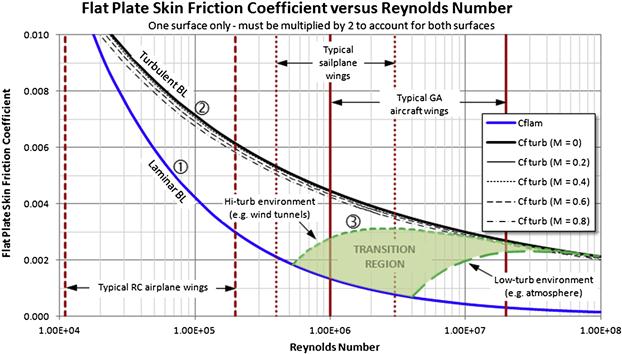
FIGURE 15-16 Change in skin friction coefficient with Reynolds number. Note the transition region, inside which it is challenging to sustain laminar boundary layer. ![]() is Equation (15-18),
is Equation (15-18), ![]() is Equation (15-19),
is Equation (15-19), ![]() is Equation (15-21).
is Equation (15-21).
Figure 15-16 also shows how susceptible to transitioning the laminar boundary layer is as it flows over a flat plate, operating within Reynolds numbers ranging from 4 × 10⁵ to 1 × 10⁷. A method to estimate this transition is presented below.
Standard Formulation to Estimate Skin Friction Coefficient
The formulation presented below is developed using boundary layer theories, such as those presented by Schlichting [4], Young [5], and Schetz and Bowersox [6]. The scope of the derivation does not lend itself to a convenient fit in this text. For this reason only results important to aircraft drag analysis are presented. The resulting relationships are plotted in Figure 15-16.
(1) Complete laminar flow: if it is assumed that laminar flow is fully sustained over a flat plate surface (a theoretical possibility only), the classical Blasius solution for a laminar boundary layer is used to estimate the skin friction:
![]() (15-18)
(15-18)
where Re = Reynolds number.
(2) Complete turbulent flow: if it is assumed that turbulent flow is fully sustained over a flat plate surface, the skin friction coefficient is given by the so-called Schlichting relation [4, p. 438], which is in excellent agreement with experiment:
![]() (15-19)
(15-19)
The skin friction coefficient for 100% turbulent boundary layer that accounts for compressibility using a variation of the Schlichting relation is given below:
![]() (15-20)
(15-20)
where M = Mach number.
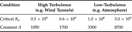
(3) Laminar-to-turbulent transition: the transition of laminar to turbulent boundary layer can be estimated using the so-called Prandtl-Schlichting skin friction formula for a smooth flat plate at zero incidence [4, p. 439], presented below. The expression is valid for Reynolds numbers up to 109.
![]() (15-21)
(15-21)
where A is read from the Table 15-1 below and is selected based on the Re at which transition is expected (critical Re).
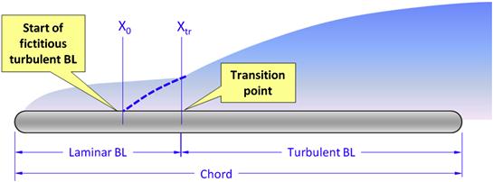
(4) Mixed laminar-turbulent flow skin friction: Young [5, pp. 162–164] presents a two-step method to calculate the skin friction coefficient when the extent of the laminar flow is known. This is the mixed laminar-turbulent theory. The first step requires the location of the transition point to be calculated:
![]() (15-22)
(15-22)
where
X0 = location of the fictitious turbulent boundary layer
Then, the skin friction coefficient is determined as follows:
![]() (15-23)
(15-23)
If the Mach number of the airplane is higher than 0.5, it is prudent to correct this value using the compressibility correction of Frankl-Voishel, presented in Equation (8-59).
It is of interest to compare Equations (15-18), (15-19), and (15-23). A good mixed boundary layer theory should bridge the gap between 100% laminar and 100% turbulent theory. In other words, when Xtr/C = 0 the result should equal the fully turbulent result and when Xtr/C = 100 it should equal the fully laminar result. Figure 15-17 shows the three theories compared. As is to be expected, the first two are constant with respect to transition location, whereas only the mixed boundary layer theory is dependent on the location of the transition point. For most Re applicable to aircraft aerodynamics it deviates only from the turbulent theory when Xtr/C < 0.06. As such, it is applicable even to turbulent boundary layer airfoils, as these will sustain laminar flow beyond 6% of the chord.

15.3.3 Step-by-step: Calculating the Skin Friction Drag Coefficient
Step 1: Determine the Viscosity of Air
In the UK system the temperature is in °R and the viscosity can be found from the following expressions [7]:
![]() (16-20)
(16-20)
In the SI system the temperature is in K and the viscosity can be found from:
![]() (16-21)
(16-21)
where
Step 2: Determine the Reynolds Number
Using Equations (8-28) through (8-30), the first one being repeated here for convenience as Equation (15-24):
![]() (15-24)
(15-24)
where
Step 3: Cutoff Reynolds Number [8]
If surface qualities are less than ideal, the actual skin friction will be higher than indicated by Equations (15-18) and (15-19). Accounting for this trend requires a special Re to be calculated, which is called a cutoff Re. If the actual Re (calculated above) is larger than this cutoff Re, then the cutoff Re should be used instead of the actual Re.
where
κ = skin roughness value (see Table 15-2)
TABLE 15-2
| Surface Type | κ (C in ft) |
| Camouflage paint on aluminum | 3.33 × 10⁻⁵ |
| Smooth paint | 2.08 × 10⁻⁵ |
| Production sheet metal | 1.33 × 10⁻⁵ |
| Polished sheet metal | 0.50 × 10⁻⁵ |
| Smooth molded composite | 0.17 × 10⁻⁵ |
(Based on Ref. [8])
Step 4: Skin Friction Coefficient for Fully Laminar or Fully Turbulent Boundary Layer
First, if the intent is to calculate the skin friction coefficient assuming a mixed boundary layer go to Step 5. Otherwise, decide whether to treat the boundary layer as either fully laminar or fully turbulent.
If it is assumed that laminar flow is fully sustained over a flat plate surface (a theoretical possibility only) calculate the skin friction coefficient using Equation (15-18):
If it is assumed that turbulent flow is fully sustained over a flat plate surface, calculate the skin friction coefficient using Equation (15-19):
If it is assumed that turbulent flow is fully sustained over a flat plate surface and subject to compressibility effects, calculate the skin friction coefficient using Equation (15-20):
![]() (15-20)
(15-20)
where
If the skin friction coefficient was calculated in this step, skip Step 5 and 6 and go directly to Step 7.
Step 5: Mixed Laminar-Turbulent Flow Skin Friction
Compute the location of the transition point using Equation (15-22):
![]() (15-22)
(15-22)
Step 6: Mixed Laminar-Turbulent Flow Skin Friction
Then, the skin friction coefficient is determined using Equation (15-23):
![]() (15-23)
(15-23)
Step 7: Compute Skin Friction Drag Coefficient
Then, the skin friction coefficient for multiple surfaces is determined as follows:
![]() (15-27)
(15-27)
![]() (15-28)
(15-28)
where
The skin friction drag force on each surface is determined using the wetted area of the individual surface as follows:
![]() (15-29)
(15-29)
Step 10: Compute the Total Skin Friction Drag Force
The total skin friction drag force on the vehicle can now be determined using the following expressions:
EXAMPLE 15-2: SKIN FRICTION DRAG OF A WING
In this example the skin friction drag of the SR22 wing will be evaluated, neglecting the interference between it and the fuselage (this is done in Example 15-6). The wing’s pertinent dimensions are shown in Figure 15-18, but these were obtained by scaling by the reported wing span of 38.3 ft. The actual wings features three distinct NLF airfoils, but for this example assume a single airfoil NACA 652-415, capable of sustaining a laminar boundary layer on the upper and lower surfaces as indicated in the figure. It is assumed that the wetted area is 7% greater than that of the shaded planform area indicated in Figure 15-18.
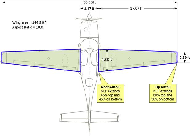
FIGURE 15-18 Scaling the top view based on the wing span yields the following dimensions (courtesy of Cirrus Aircraft).
If the airplane is cruising at 185 KTAS at S-L ISA, determine the skin friction drag coefficient and force acting on the wing due to the mixed laminar and turbulent BL regions. Compare to a wing with fully laminar or fully turbulent BL.
Solution
Note that the solution below was calculated using the spreadsheet software Microsoft Excel. The reader entering the numbers into a calculator will probably notice slight difference from the numbers shown. This is normal and is due to the fact that Microsoft Excel retains 16 significant digits whereas the typical calculator retains 8 significant digits, not to mentioned user round-off differences.
Step 1: Determine the Viscosity of Air
Use Sutherland’s formula to compute the viscosity assuming an OAT of 518.67 °R:

Step 2: Determine the Reynold’s Number for Root Airfoil
Compute Re for the root airfoil, using ISA density of 0.002378 slugs/ft3 and an airspeed of 185 KTAS.
![]()
Step 3: Determine the Reynold’s Number for Tip Airfoil
Compute Re for the tip airfoil:
![]()
Step 4: Fictitious Turbulent BL on Root Airfoil – Upper Surface
For the upper surface of the root airfoil (45% coverage) we get:
![]()
Step 5: Fictitious Turbulent BL on Root Airfoil – Lower Surface
For the lower surface of the root airfoil (45% coverage) we get the same value as on the upper surface:
![]()
Step 6: Fictitious Turbulent BL on Tip Airfoil – Upper Surface
For the upper surface of the tip airfoil (60% coverage) we get the same value as on the lower surface:
![]()
Step 7: Fictitious Turbulent BL on Tip Airfoil – Lower Surface
For the lower surface of the tip airfoil (50% coverage) we get:
![]()
Step 8: Skin Friction for Root Airfoil – Upper Surface
For the upper surface of the root airfoil (45% coverage) we get:
![]()
Step 9: Skin Friction for Root Airfoil – Lower Surface
For the lower surface of the root airfoil (45% coverage) we get:
![]()
Step 10: Average Skin Friction for Root Airfoil
The average of the upper and lower surfaces of the root airfoil yields:
![]()
Step 11: Skin Friction for Tip Airfoil – Upper Surface
For the upper surface of the tip airfoil (60% coverage) we get:
![]()
Step 12: Skin Friction for Tip Airfoil – Lower Surface
For the lower surface of the tip airfoil (50% coverage) we get:
![]()
Step 13: Average Skin Friction for Tip Airfoil
The average of the upper and lower surfaces of the tip airfoil yields:
![]()
Step 14: Average Skin Friction for Complete Wing
The skin friction coefficient for the total wetted surface is simply the average of the average coefficient for both airfoils, i.e.:
![]()
Step 15: Wing’s Wetted Area
The wing’s total wetted area is:
![]()
Step 16: Skin Friction Drag Coefficient for Complete Wing
The wing’s skin friction drag coefficient is:
![]()
Step 17: Skin Friction Drag Force for Complete Wing
Estimate skin friction drag due to the mixed boundary layer.
![]()
This means that the total flat plate skin friction drag for the wing only of the SR22 at cruising speed amounts to 63 lbf. The contributions of interference with the fuselage and airfoil shape are not accounted for. It also omits drag due to the presence of control surfaces.
Step 19: Skin Friction Coefficient for 100% Turbulent Flow
Turbulent flow coefficient for the root:
![]()
Turbulent flow coefficient for the tip:
![]()
Step 20: Comparison
See Table 15-3 for a comparison of the the analysis techniques.
TABLE 15-3
Comparing Skin Friction Analysis Methods
| Method | Cf | Comparison |
| Fully Laminar BL | 0.0005068 | 25% |
| Fully Turbulent BL | 0.003185 | 159% |
| Mixed BL | 0.001999 | 100% |
The most important observation from this comparison is that if it were possible to maintain laminar flow over the entire wing, its drag would be 25% of that predicted by the mixed boundary layer theory. Naturally, this is impossible to achieve, but rather represents an extreme. Alternatively, if the wing sustained turbulent BL only, it would be almost 60% draggier than with the NLF airfoils. This represents a far more realistic comparison and demonstrates the value of employing such airfoils.
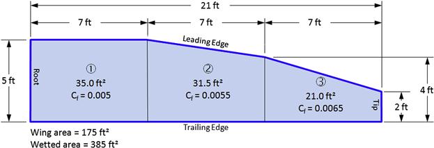
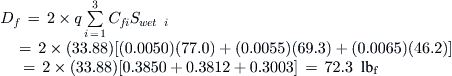
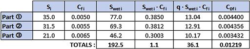
EXAMPLE 15-3: TOTAL SKIN FRICTION OF A MULTI-PANEL WING
A halfspan of a Schuemann style wing is shown in Figure 15-19. The planform consists of three sections with the dimension and the total wing and wetted areas shown. The skin friction coefficient for each section has been determined and is tabulated with the corresponding planform areas. If this wing (the full wing) is exposed to S-L conditions at 100 KCAS and using the wing area as the reference area and assuming the wetted area is 2× the surface area multiplied by a wetted area booster factor, Kb, of 1.1, estimate the following:
Total skin friction coefficient
Total skin friction drag coefficient
Solution
(a) Begin by creating Table 15-4 as follows (where Swet i = 2 × Kb × Si). Thus, the wetted area for panel ![]() is given by Swet
is given by Swet ![]() = 2 × Kb × S
= 2 × Kb × S![]() = 2 × (1.1) × (35.0) = 77.0 ft2. Subsequent multiplication using Cf
= 2 × (1.1) × (35.0) = 77.0 ft2. Subsequent multiplication using Cf ![]() = 0.0050 and q = ½ρV2 = ½ (0.002378)(100 × 1.688)2 = 33.88 lbf/ft2 yield the other two columns. Next, the totals of the three right-most columns are calculated. Note that these are for only one of the two wing halves.
= 0.0050 and q = ½ρV2 = ½ (0.002378)(100 × 1.688)2 = 33.88 lbf/ft2 yield the other two columns. Next, the totals of the three right-most columns are calculated. Note that these are for only one of the two wing halves.
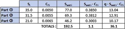
Then the total skin friction coefficient can be found by the weighted contribution from each panel:
![]()
This should be considered the representative skin friction coefficient for the wing. Note that the application of form factors is not needed when accounting for each panel as all the panels belong to the same unit.
(b) The total skin friction drag coefficient is always based on the reference area, here chosen as the wing area Sref = 160 ft2:
![]()
This amounts to 121.9 drag counts.
(c) And (d) since the skin friction coefficient differs from one panel to the next, the drag force on each surface must be determined using the wetted area of the individual surface as follows:
![]()
Therefore the total skin friction drag force for both wing halves can be found by summing up the individual contributions:
or:
![]()
or:
![]()
We can also calculate the skin friction drag coefficient, CDfi, for each panel for each wing half (assuming only half of the reference wing area) as shown below. Note the results are presented in Table 15-5.
![]()
![]()
![]()
In calculating the above drag, two important influences were neglected: form and interference effects. A form effect comes from the fact that more information than just wetted area is required to correctly estimate the drag of the component. This is easy to realize when comparing a sphere or a box of equal wetted area. Intuitively it is obvious to us that the drag of the box will be higher than that of the sphere. This effect is accounted for using the so-called form factor, to be dealt with later. Also, when calculating the combined effect of panels comprising a larger surface (such as the wing in the above example) there are no specific interferences that have to be considered. In other words, the proximity of components when mounting a wing to a fuselage or a horizontal tail to a vertical tail, and so on, affects the drag. This effect is called an interference drag and it increases the drag beyond what the above example indicates. Interference is accounted for using a so-called interference factor. Both the form and interference factors account for the effects of viscous separation (pressure drag) and are evaluated in Section 15.4.6, The component drag build-up method. In particular see Example 15-6.
15.3.4 The Lift-Induced Drag Coefficient: CDi
Consider a finite wing featuring a single airfoil mounted in space in airflow at some specific AOA and airspeed. Contrast that with a straight wing featuring exactly the same airfoil, extending from wall to wall in a wind tunnel at the same AOA and airspeed (ignoring typical wind-tunnel interferences). In this situation, the finite wing will generate less lift per unit span than the one in the wind tunnel. This is caused by the fact that the airflow makes its path around the wingtips of the finite wing through the formation of vortices, one at each wingtip. The short consequence of this flow is that in order for the wing to generate a specific amount of lift, it must always be at a higher AOA than the corresponding two-dimensional airfoil in the wind tunnel. This leads to the formation of drag that increases the wing drag beyond that of the airfoil only. This drag is called a lift-induced, or induced, or vortex drag and is denoted by Di. As usual the standard formulation of this drag involves the determination of a lift-induced drag coefficient. A number of methods to determine this drag coefficient are presented below. The lift-induced drag is a pressure drag force.
Method 1: Lift-Induced Drag from the Momentum Theorem
A wing can be considered a device that generates lift by deflecting a stream of fluid downward; an event that changes the fluid’s momentum. The downward motion of the fluid is called downwash. The magnitude of this lift can be estimated using Newton’s second law of motion, which states that force is the rate of change of momentum. In doing so it is assumed the diameter of the stream tube being deflected equals the wingspan,4 denoted by b. The mass flow rate inside this cylinder is denoted by ![]() . If the vertical downwash at some distance behind the wing is denoted by w, the rate of change of momentum (lift force) can be estimated from:
. If the vertical downwash at some distance behind the wing is denoted by w, the rate of change of momentum (lift force) can be estimated from:
![]() (15-32)
(15-32)
The mass flow rate in the stream tube is given by ![]() , where Atube is the cross-sectional area of the stream tube. Thus, the lift can be rewritten as follow:
, where Atube is the cross-sectional area of the stream tube. Thus, the lift can be rewritten as follow:
![]() (15-33)
(15-33)
Equating this with the standard expression for lift (Equation (8-8)) allows the magnitude of the downwash to be estimated:
![]() (15-34)
(15-34)
![]() (15-35)
(15-35)
This is shown in Figure 15-20. The circulation of fluid around the airfoil will cause a reduction in the geometric AOA, denoted by α, which is the angle between the flight path and chordline. The reduction is called induced AOA and is denoted by αi. The circulation introduces an upwash into the airflow (and downwash behind it), reducing the geometric AOA. The difference between the two is called the effective AOA, denoted by αe. It can be seen that the downwash angle will be given by w/V and that αi is approximately one-half of that angle. For this reason, using Equation (15-35) and small-angle relations, we can estimate the induced AOA as follows:
![]() (15-36)
(15-36)
Then, again referring to Figure 15-20, it can be seen that the presence of the induced AOA effectively tilts the lift force back by that amount, in the process forming an additional force component Di, which we call lift-induced drag. This drag can be calculated as shown in the figure.
![]() (15-37)
(15-37)
The above derivation is based on the assumption that the lift distribution is elliptical or, in other words, the spanwise distribution of section lift coefficients is constant. As has been shown in Chapter 9, The anatomy of the wing, this requires an elliptical planform. However, most wing planform shapes are not elliptical and, consequently, the distribution of section lift coefficients is far from being constant. This requires corrections to be made. Such corrections are discussed below.

The following representation of the lift-induced drag is of importance from an aircraft design standpoint. Using Equation (15-38) to determine the induced drag force yields:
![]() (15-39)
(15-39)
The result shows that the lift-induced drag force depends on the wing span and not the wing area. This means that only an increase in span will have beneficial effect on the drag. Reducing the chord to increase AR will not help.
Method 2: Generic Formulation of the Lift-Induced Drag Coefficient
Generic formulation of wing characteristics is presented in NACA-TR-572 [9], based on the work of Glauert [10] and Hueber [11]. It allows a number of wing characteristics to be evaluated for tapered wing planform shapes, with and without rounded wingtips (which were popular during the time when it was written). A generic formulation of the lift-induced drag, CDi, is presented as follows:
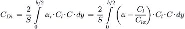 (15-40)
where
A more general version of this expression is possible, which can treat asymmetric wing loading. It is presented below:
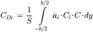 (15-41)
Derivation of Equation (15-40)
The induced AOA at any section along the wing can be computed if the section lift coefficient, Cl, and section lift curve slope, Clα, are known:
![]() (15-42)
(15-42)
Therefore, using small-angle relations, the induced drag of the airfoil section can be computed from:
![]() (15-43)
(15-43)
The total lift-induced drag for the wing will then be the sum of the weighted contribution of all the sections, extending from tip to tip, or:
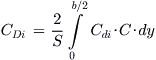 (15-44)
The weighted form is necessary as the planform shape is may be changing or affected by washout. This way, multiplying it with the chord, C, Inserting the result from Equation (15-43) and manipulate will yield Equation (15-40).
QED
EXAMPLE 15-4
Estimate the induced drag coefficient for a Hershey bar wing with the following characteristics:
The wing is operating at an AOA = 5° = 0.08727 radians and it has been determined its spanwise distribution of section lift coefficients can be approximated by Cl = 0.5·cos(πy/b) and is shown in Figure 15-21. The wing features an airfoil whose Clα = 5.730 per radian and is untwisted.
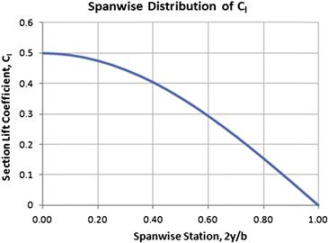
Solution
Solution is obtained by evaluating the integral of the distribution of the section lift coefficients along the entire span of the aircraft per Equation (15-40):
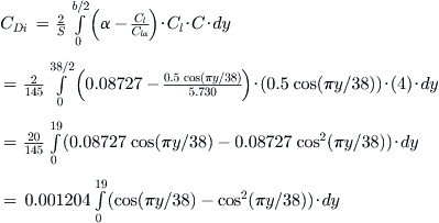
![]()


Method 3: Simplified k·CL2 Method
This is the simplest representation of lift-induced drag. As has already been demonstrated, it can be derived directly from the momentum theorem, or using the lifting line method presented in Section 9.7, Numerical analysis of the wing.
![]() (15-45)
(15-45)
where
The most difficult parameter to determine is the Oswald efficiency. It can be estimated using Method 5 below. Several methods to estimate it are also provided in Section 9.5.14, Estimation of Oswald's span efficiency. Note an important dependency of the induced drag coefficient on wing area, S, and wing span, b:
![]() (15-46)
(15-46)
This result shows that for a given wing area, S, the induced drag is highly dependent on the wing span. It is an important consideration for many applications that feature large area but small wingspan (e.g. a delta wing).
Method 4: Adjusted k·(CL − CLminD)2 Method
As has already been emphasized in the preceding discussion, the adjusted drag model is a far more accurate method of lift-induced drag estimation than the simplified model. This model is presented below:
![]() (15-47)
(15-47)
where CL minD = the lift coefficient where drag becomes a minimum.
Method 5: Lift-Induced Drag Using the Lifting-Line Method
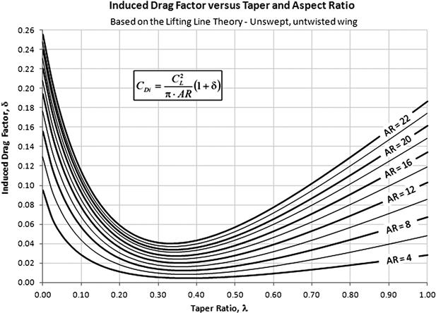
In order to remedy the difficulty in determining the lift-induced drag constant, k, shown in Equations (15-7), (15-45), and (15-46), numerical methods, such as the lifting-line or vortex-lattice methods, may be used. Of the two, the lifting-line method, presented in Section 9.7, Numerical analysis of the wing, is relatively easy to apply, although it requires a matrix solver to calculate the constants of simultaneous linear equations. These are then used to evaluate a special constant, called the lift-induced drag factor, denoted by the Greek letter δ. Once this is known, the lift-induced drag coefficient can be calculated from:
Figure 15-22 shows the variation of the lift-induced drag factor, δ, with a range of taper ratios, λ, and aspect ratios, AR, as calculated by the lifting-line method presented in Section 9.7. A code snippet, using Visual Basic for Applications, is also presented in the section, allowing the reader to determine the factor using software such as Microsoft Excel. Note that the Oswald’s span efficiency, e, is related to the lift-induced drag factor as shown below:
![]() (15-50)
(15-50)
EXAMPLE 15-5
The SR22 has an AR = 10 and a λ = 0.5. If flying at a condition that generates a CL = 0.5, determine the lift-induced drag coefficient using Figure 15-22. For this example, assume CLminD = 0.
Solution
From Figure 15-22 it can be seen that δ ≈ 0.022. This means that the lift-induced drag coefficient can be determined as follows:
![]()
This value is 2.2% higher than that for an elliptical wing of the same AR.
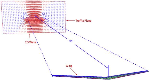
Method 6: Prandtl-Betz Integration in the Trefftz Plane
This method was developed by Ludwig Prandtl (1875–1953) and Albert Betz (1885–1968) around the year 1918. The method computes the induced drag of a wing based on disturbance it causes to the fluid flow in the far-field (see Figure 15-23). By evaluating the disturbances on a plane infinitely behind the wing (Trefftz plane, named after Erich Trefftz (1888–1937)), the velocity component in the x-direction (denoted by u) can be eliminated from the integration. In this way, a volumetric integration can be reduced to a surface integration.
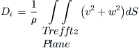 (15-51)
The method is often applied using computational fluid dynamics (CFD) methods, such as the vortex-lattice method, and is primarily presented here for completeness.
15.3.5 Total Drag Coefficient: CD
Once the constituent drag contributions have been estimated, the total drag coefficient is simply determined by addition using the following expression:
![]() (15-52)
(15-52)
Note that the combination CDo + CDf is highly internally dependent and, therefore, in this book, they are combined and called the minimum drag, CDmin. However, in light of the above definition, inserting the explicit forms of the other coefficients yields:
![]() (15-53)
(15-53)
For internal consistency it is better to write:
![]() (15-54)
(15-54)
15.3.6 Various Means to Reduce Drag
As has already been stated, drag is generally a detrimental force in aircraft design, in particular for operational missions that require fuel efficiency. In addition to “obvious” means to reduce drag, such as retractable landing gear and smooth NLF surfaces, people have been creative in their attempts to reduce drag. Below are a selected number of ideas conceived with this intent, presented here to inspire the reader.
Reduction of Drag on Wings via Laminar Flow Control (LFC)
The history of LFC dates back to 1930s and is well documented by Chambers [12] and in particular Braslow [13]. LFC is also referred to as artificial laminar flow (ALF) to contrast with natural laminar flow (NLF). LFC is an attempt to maintain the laminar boundary layer over a large part of the wing by effectively “sucking” the turbulent boundary layer through tiny perforations in the wing skin. A variation of LFC, called hybrid LFC or HLFC, uses NLF for a larger portion of the wing to reduce the power required to eliminate the turbulent boundary layer growth. The primary drawback of such methods is that they are active rather than passive. In other words, additional energy is required to lower the pressure inside the wing and draw in the external boundary layer. Furthermore, it is a serious detriment that the perforations negatively affect the structural integrity of the wing and the operator must deal with nuisances such as cleaning the remains of insects that can clog the perforations, reducing system performance.
Figure 15-24 shows the difference in airflow over an airfoil with and without LFC. The left photo shows the airfoil at an AOA of 20° and clearly shows fully separated wake behind it. The right photo shows the same airfoil with the LFC turned on. The change in the nature of the flow is clearly evident, with the separation being eliminated as far aft as 70% of the chord. This “unstalls” the airfoil, giving it a higher Clmax, in addition to a reduction in drag. It demonstrates the promising potential of LFC technology, although being severly hampered by a number of factors, as is discussed in Ref. [12].

FIGURE 15-24 The effect of laminar flow control. The AOA is approximately 20°. (Photos by Phil Rademacher)
An early example involves the Northrop X-21A, which was a heavily modified Douglas WB-66D aircraft. Its two original Allison J71 engines, originally on the wing, were replaced with two GE XJ79s that were mounted to the rear fuselage. The bleed air from these engines was then used to drive a compressor that, effectively, sucked the wing boundary layer through slots in the wing. The system, while demonstrating LFC was effective, turned out to be a manufacturing and maintenance nightmare and too costly to be practical.
In 1999, Marshall [14] investigated the effectiveness of a variable-porosity suction glove on the F-16XL-2 aircraft to demonstrate the feasibility of boundary layer suction for supersonic operation. The research showed that at the test condition of Mach 2 at 53000 ft (Re of the order of 22.7 × 10⁶) the laminar boundary layer was sustained as far aft as 46% of the chord.
Finally, van de Wal [15] showed merely 3.2% reduction in total drag of a small GA aircraft (ENAER Namcu), reporting that installing a boundary layer suction system was not beneficial to its operation.
Winglets
Winglets and the potential for a reduction in lift-induced drag are discussed in Section 10.5.7, The winglet.
NLF Airfoils
Natural Laminar Flow airfoils are an obvious choice when trying to reduce drag. Of course they have to be selected before the airplane is built. NLF airfoils are discussed in great detail earlier in this chapter and Chapter 8, The anatomy of the airfoil.
Reduction of Drag of Fuselages
Wortman [16] suggests that the installation of relatively large fixed-pitch vortex generators on the bottom near the beginning of the upsweep of the lower fuselage of transport aircraft can reduce the total drag by 1–2%. The idea was validated in extensive wind tunnel tests using fuselage models of the Boeing 747 and Lockheed C-5 Galaxy transport aircraft. The author suggests the vortex generators can be installed on such aircraft for a fraction of the cost of their monthly operational cost. Such vortex generators are shown mounted to the aft lower fuselage of the B-52 Stratofortress in Figure 15-25.
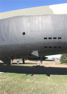
FIGURE 15-25 Vortex generators on the aft fuselage of a B-52 Stratofortress. (Photo by Phil Rademacher)
Kentfield [17] suggests that using a stepped after-body can significantly reduce the drag of an axis-symmetric fuselage style bodies. The unorthodox idea is to allow an entrapped vortex to form at each step of the conical after-body, which allows the airflow to better follow its geometry, ultimately reducing its drag. The method is unorthodox and results in an unusual after-body geometry that would be hard to justify from an aesthetics standpoint, not to mention there could be some structural challenges.
A clear way to reduce fuselage drag is to employ tadpole fuselages, like those used for sailplanes. Naturally, such fuselages are not always practical considering the mission of the airplane. Tadpole fuselages are discussed in Appendix C4, Design of sailplanes, and Section 12.2.3, The tadpole fuselage.
In evaluating the importance of smooth surfaces in maintaining NLF on lifting surfaces (wing, HT, and VT), Quast and Horstmann [18] demonstrate the magnitude of fuselage drag. Using the Airbus 300 as an example, they estimate the drag of the fuselage alone amounts to about 49% of the minimum drag. Studies of this nature are an important reminder that it is easy to spend a tremendous amount of effort getting a few drag counts out of the lifting surfaces, while overlooking the greatest source of drag altogether – the fuselage.
Reduction of Drag of the Fuselage/Wing Juncture
The juncture of the fuselage and wing can be particularly bothersome as it is not always easy to estimate tendency for flow separation. Due to steep adverse pressure gradients that often result in the region such separation can occur even at low AOAs. The implication is increased drag during climb and even cruise and thus reduced performance.
Modern methodologies are being developed that use state-of-the-art Navier-Stokes computational fluid dynamics (N-S CFD) tools to shape the wing fairing using genetic algorithms. Peigin and Epstein [19] suggest the use of such tools and demonstrated a 43 drag count drag reduction in a before-and-after investigation of a business jet.
15.4 The Drag Characteristics of the Airplane as a Whole
For some, the pinnacle of aircraft design is the estimation of the drag of the whole airplane. We have already discussed the shortcomings of such analyses and emphasized enough the care that must be exercised. In this section methods will be presented to estimate the drag of the new design. We will use the Cirrus SR22 as an example by evaluating its drag and comparing it to the drag coefficient that can be extracted from published performance data (i.e. POH values obtained through certification flight testing).
The ideal airplane designed for cruise should be designed to operate near or at its minimum drag coefficient, CDmin. This is actually hard to accomplish in practice, but is still the goal. If this can be achieved, practically any deviation from this condition will increase the drag of the airplane: changing the airspeed will change the AOA and increase the drag coefficient; moving the CG to a new position (if possible) will also increase the drag coefficient, as will deflecting the control surfaces. We can expand on this imaginary situation by considering changes in surface smoothness, addition of inlets and outlets, antennas, and the like, all which will increase the drag. Such a thought exercise helps the realization that drag is inherently hard to reduce but easy to increase. The aspiring designer must anticipate this effect while attempting to manage and resist requests for features from many directions; typically from management, potential customers, systems group, and similar.
Many effects of some specific sources of drag on the aircraft have already been presented in Chapter 8, The anatomy of the airfoil. Here, we will only add ones that are specifically limited to three-dimensional aircraft.
15.4.1 The Effect of Aspect Ratio on a Three-Dimensional Wing
In 1923, Prandtl [20] presented the results of well-known experiment which depict well the effect aspect ratio has on the generation of lift and drag of a wing. A copy of of his actual results is shown in Figure 15-26. The graph to the right shows what has already been discussed in Chapter 9, The anatomy of the wing, the impact of AR on lift. The graph to the left shows the effect of AR on drag. It shows that two wings (call them Wing 1 and Wing 2) whose geometry differs only in the AR (wing area and airfoil, and thus the minimum drag of the airfoil, Cdmin, are assumed the same) will generate drag coefficient at the same CL, which can be expressed as follows:
![]() (15-55)
(15-55)
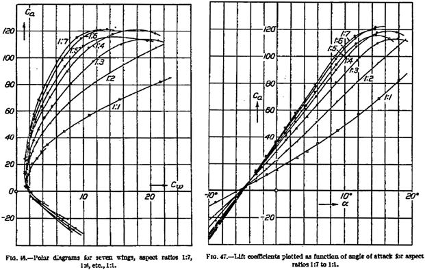
FIGURE 15-26 Ludwig Prandtl’s original research demonstrates how lift and drag of a wing change with aspect ratio. (from Ref. [20])
From this it is evident if the drag of one wing, say Wing 1, is known, the drag of the other one can be estimated from the difference of the two drag polars:
![]() (15-56)
(15-56)
Of course, the expression holds as long as the difference in the ARs is not too great. This is because the chord length of the airfoil will affect the minimum drag of the airfoil, Cdmin, and the AR will affect the Oswald span efficiency factor, e.
Figure 15-27 shows the effect of changing the AR of a three-dimensional wing on the drag polar using modern notation of coefficients. It shows that as the magnitude of the aspect ratio does not change the minimum drag (not accurate if the change is large), but rather the width of the drag polar is reduced. This is a consequence of a reduction in the magnitude of the CLmax and the lift curve slope, CLα. The reduction is easily estimated through the use of Equations (15-38), (15-45), and (15-47).
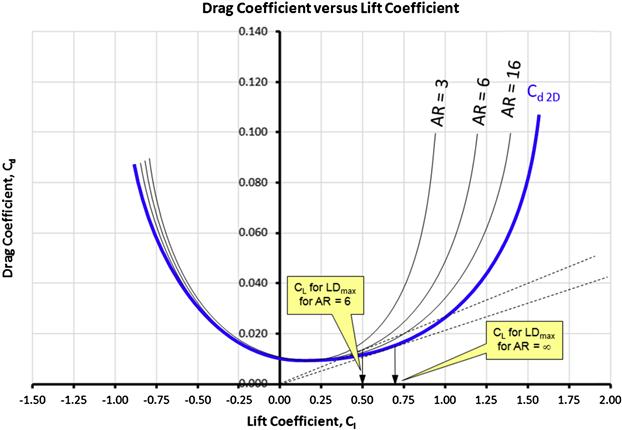
FIGURE 15-27 The effect of different values of the AR on the drag polar assuming S = constant. (based on Ref. [20])
15.4.2 The Effect of Mach Number
Generally, as the airplane approaches the speed of sound, the drag coefficient will begin to rise sharply. The Mach number at which the rise begins depends on the geometry of the airplane. An airplane with thick airfoils will experience it perhaps as early as M = 0.6, whereas a sleek high performance jetliner begins to experience it at M ≈ 0.85. This rise is handled in the drag estimation by the addition of a compressible drag coefficient, ΔCDC, which is most accurately estimated in wind tunnel testing or by sophisticated CFD methods. The Mach number at which this happens is called the drag-divergence Mach number, denoted by Mdd, and it occurs slightly above the critical Mach number (see Section 8.3.7, The critical Mach number, Mcrit).
The drag-divergence Mach number is defined either when ΔCDC = 0.002 or when dCDC/dM = 0.10.
Figure 15-28 shows a hypothetical scenario in which an airplane flying at a constant CL experiences a sharp rise in the compressible drag coefficient near M = 0.7. As stated earlier, this is the critical Mach number, denoted by MCRIT. Its value largely depends on the geometry of the aircraft and details such as the thickness of the wing airfoils and the geometry of the wing/fuselage juncture, to name few. In fact, any part of the airplane which features interferences due to the joining of disparate components is suspect. Such interferences typically result in increased local airspeeds, which promote the formation of normal shocks (and therefore higher drag) in the juncture.
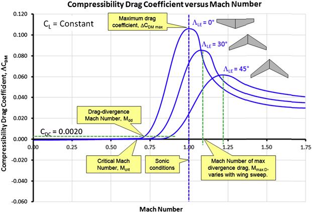
A method to estimate this contribution to the total drag is presented in the Section 15.5.12, Drag due to compressibility effects.
15.4.3 The Effect of Yaw Angle β
As discussed in Section 15.3.4, The Lift-Induced Drag Coefficient: CDi, drag varies greatly with AOA. This effect extends to yaw as well, as shown in Figure 15-29; it too increases the drag and is usually minimum when β = 0°. This fact has been used for a long time by pilots when landing. Pilots “coming in too high” for a landing will yaw the airplane, decreasing its L/D ratio, allowing the airplane to temporarily lose altitude more rapidly. This addition depends entirely on the geometry of the aircraft. Generally, it is an acceptable approximation to assume the flow to stay attached on the aircraft for a β up to ±10°. However, beyond that, flow separation is certain and the associated drag increase must be accounted for.
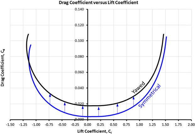
15.4.4 The Effect of Control Surface Deflection – Trim Drag
Deflecting control surfaces usually increases the drag of the aircraft. For instance, deflecting the elevator shifts the drag polar vertically, increasing the CDmin. This change is referred to as the trim drag. If a conventional tail-aft airplane is loaded with its CG far forward, a higher deflection of the elevator will be required to trim it. This implies additional drag, in addition to the extra lift the wing must generate that increases lift-induced drag. This is why it is important to size the tail so the elevator is close to neutral in cruise (usually referred to as an elevator “in trail”).
Trim drag is most accurately estimated using precise wind tunnel tests, although it can certainly be estimated using analytical methods too. A graph similar to the one in Figure 15-30 is usually obtained, with several curves showing the drag polar for an elevator deflection of, say, 0°, 2°, 4°, 6°, 10°, and so on. These allow the performance engineer to better estimate the capability of the airplane at different loading and flight conditions. In the absence of wind tunnel testing, it is imperative to be able to assess it with some level of accuracy, in particular if the airplane features a high (or low) thrustline.

A method to estimate trim drag based on CG location and thrust setting is presented in Section 15.5.2, Trim drag.
15.4.5 The Rapid Drag Estimation Method
The rapid drag estimation method is without question the fastest way to estimate the drag of an airplane. It is based on the assumption that there is a correlation between the averaged skin friction coefficient of an airplane, its total wetted area, and its minimum drag coefficient. Naturally, with this speed comes inaccuracy, so the method should only be used to figure out a “ballpark” value for the drag to compare to other methods. For instance, the method does not account for any peculiarities in the airplane design, such as extent of laminar flow, specific geometric features, and others. It is possible to account for the rudimentary effects of flaps and landing gear, but again, the designer should not use this method for anything but to get an idea of the magnitude of the drag coefficient, and not be surprised if it is vastly different from the value obtained by more accurate methods. The method calculates the minimum drag coefficient using the concept of EFPA (see Section 15.2.2, Quadratic drag modeling) and Equation (15-8):
![]() (15-57)
(15-57)
where
The method involves reading the value of f for a “clean” aircraft from Figure 15-31, using the approach outlined in the figure. Ideally, the estimate of the aircraft’s wetted area should be as precise as possible. Also note that the equivalent skin friction coefficient means a normalized value representative for the entire aircraft. It is inevitable, considering the variety in the surface quality of a normal airplane, that some engineering judgment will be required to assess the value.
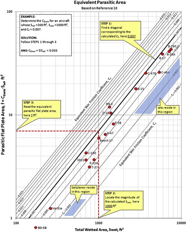
The drag increments due to flaps, landing gear, speed brakes, etc., are accounted for using the following relation and then added to the CDmin:
![]() (15-58)
(15-58)
where
The equivalent parasite areas and coefficients are obtained from the Table 15-6, where AC stands for maximum cross-sectional area, Sref is the wing reference area and SHT is the HT planform area.

15.4.6 The Component Drag Build-Up Method
The component drag build-up method (CDBM) is used to estimate the drag of the complete aircraft. The method is primarily based on the estimation of flat plate skin friction over the surfaces of the airplane that are exposed to the airflow (wetted area). The method accounts for geometric differences between components and changes in drag resulting from bringing one component into the neighborhood of another (interferences).
The CDBM bases the parasitic drag (the combination of CD0 + CDf) using flat plate skin friction coefficients that are modified using two special factors called a component form factor (FF) and interference factor (IF). The FF is a measure of the pressure drag due to viscous separation. It accounts for the fact that the drag force generated by a sphere and a box of equal wetted area is different from one another. Interference effects between aircraft parts (wing and fuselage, engine and wing, HT and VT, etc.) are accounted for using a special factor called component interference factor (IF). This factor is based on the fact that as two bodies are brought together in fluid flow, the drag of the combination is greater than the drag of the individual bodies on their own. The IF is denoted by Q in Raymer, but by IF by most other authors.
A flow chart showing the procedure is shown in Figure 15-32. In the flow chart, the “+” sign means that contributions are added, whereas the “×” sign means multiplication.

FIGURE 15-32 Flow chart describing the component drag build-up method. Recall that CDf i = Cf i·(Swet i/Sref).
The method requires the skin friction coefficients to be calculated for all components in direct contact with air (or wetted by air) ![]() . The components are parts like the wings, horizontal tail, vertical tail, and so on. Even though the wing, HT, VT, and fuselage are shown, other components, such as engine nacelles, pylons, winglets, external fuel tanks, dorsal, or ventral fins, should be added to the list if present. Naturally, they should be excluded only if other means to estimate their drag is selected (e.g. see Section 15.5, Miscellaneous or additive drag) and then be included as miscellaneous drag, CDmisc. These are adjusted with FF
. The components are parts like the wings, horizontal tail, vertical tail, and so on. Even though the wing, HT, VT, and fuselage are shown, other components, such as engine nacelles, pylons, winglets, external fuel tanks, dorsal, or ventral fins, should be added to the list if present. Naturally, they should be excluded only if other means to estimate their drag is selected (e.g. see Section 15.5, Miscellaneous or additive drag) and then be included as miscellaneous drag, CDmisc. These are adjusted with FF ![]() through a multiplication operation, but this ensures dissimilar components don’t contribute equally to the overall drag even if both have identical wetted areas. Then, IFs are applied
through a multiplication operation, but this ensures dissimilar components don’t contribute equally to the overall drag even if both have identical wetted areas. Then, IFs are applied ![]() , also through a multiplication operation, to account for the increase in drag when individual components are brought into close proximity.
, also through a multiplication operation, to account for the increase in drag when individual components are brought into close proximity.
Once the skin friction drag (with its associated pressure and interference drag boosting) has been determined, the next step is to determine all remaining sources of drag. This is simply called miscellaneous or additive drag ![]() . This is drag attributed to miscellaneous sources, such as antennas, fuel caps, air flow through small gaps (such as those between control surfaces and the lifting surface to which they are mounted), as well as control system components (bellcranks, hinges, etc.), inlets, outlets, antennas, and so on. These are then summed up and multiplied by a crud-factor
. This is drag attributed to miscellaneous sources, such as antennas, fuel caps, air flow through small gaps (such as those between control surfaces and the lifting surface to which they are mounted), as well as control system components (bellcranks, hinges, etc.), inlets, outlets, antennas, and so on. These are then summed up and multiplied by a crud-factor ![]() , which accounts for contributions that are practically impossible to account for otherwise, such as surface panel misalignments, dents, small vents and outlets, and so on. The crud factor is typically 25%, which means that the sum of the above contributions is multiplied by 1.25. This operation returns the minimum drag coefficient
, which accounts for contributions that are practically impossible to account for otherwise, such as surface panel misalignments, dents, small vents and outlets, and so on. The crud factor is typically 25%, which means that the sum of the above contributions is multiplied by 1.25. This operation returns the minimum drag coefficient ![]() . We add to it the lift-induced drag coefficient at the flight condition
. We add to it the lift-induced drag coefficient at the flight condition ![]() to obtain the total drag coefficient
to obtain the total drag coefficient ![]() .
.
The total component drag build-up is expressed as follows:
![]() (15-59)
(15-59)
where
15.4.7 Component Interference Factors
As previously stated, interference factors (IF) are used to account for the proximity of one component to another. For instance consider the juncture between the wing and fuselage. The presence of both bodies constrains the airflow compared to that of the individual components, increasing the local airspeeds greatly, which increases the drag. However, this does not account for additional drag that may arise due to early separation due to a poorly designed wing/fuselage juncture.
Table 15-7 lists typical IFs that are partially derived from Refs [3] and [25] and partially using factors that have worked well in drag analyses performed by the authors. No claim is made about their accuracy beyond that. Note that when using the factors for multiple objects, for instance, a triple-tail, the presented IF must be applied to all surfaces. Thus, when summing up the four surfaces of such a tail (one HT and three VTs), their corresponding CDf (= Cf i·(Swet i/Sref)) must be multiplied each time. The following formulation illustrates how its contribution would be accounted for in the CDBM:
![]()
TABLE 15-7
| Component | IF |
| Nacelle or external store, directly under a fuselage | 1.5 |
| Nacelle or external store, under a fuselage, less than about 1 diameter away | 1.3 |
| Nacelle or external store, under a fuselage, more than about 1 diameter away | 1.0 |
| Object, such as a fuel tank, mounted to a wingtip | 1.25 |
| High wing or mid wing with carefully designed fairing | 1.0 |
| Un-filleted low wing | 1.1–1.4 |
| Whitcomb winglet | 1.04 |
| “Airbus” style winglet | 1.04 |
| Modern blended winglet | 1.00–1.01 |
| Aerodynamic or square leaf-spring main landing gear strut entering wing or fuselage | 1.10 |
| Aerodynamic wing strut entering wing on one end and fuselage on the other | 1.10 |
| Boundary layer diverter | ∼1.0 |
| Conventional tail | 1.04–1.05 |
| Cruciform tail | 1.06 |
| V-tail | 1.03 |
| H-tail (B-25 Mitchell or A-10 Warthog style) | 1.08 |
| H-tail (Lockheed Model 10 Electra style) | 1.13 |
| H-tail (Beech D-18 style) | 1.06 |
| Triple-tail (Lockheed Constellation style) | 1.10 |
| T-tail | 1.04 |
15.4.8 Form Factors for Wing, HT, VT, Struts, Pylons
As stated earlier, a form factor (FF) reflects the geometric shape of components and, therefore, methods to estimate this value varies greatly with classes of components. Thus there is a set of FFs that are only used with geometry capable of generating lift (“wing-like” surfaces). Others are only used with geometry that serves as fuselages, and so on. The following expressions are used to estimate FF for lift for wing-like surfaces. Such surfaces include wings, horizontal tail, vertical tail, struts, and pylons, but can also be extended to wing-shaped antennas and landing gear pant fairings. These form factors are typically derived by semi-empirical methods that emphasize the thickness-to-chord ratio of the structure. The following form factors are found in the literature.
The inevitable question that comes up is “which one do I pick?” Unless a specific application is cited (like the ones by Hoerner) the answer is often based on engineering judgment. In that case the unsure designer can take the average of two or three methods.
Hoerner [3, p. 6-6] suggests the following form factors for lifting surfaces featuring airfoils whose (x/c)max = 30%:
![]() (15-60)
(15-60)
Hoerner [3] suggests the following form factors for lifting surfaces featuring airfoils whose (x/c)max = 40% to 50%, such as NACA 64 and 65 series airfoils:
![]() (15-61)
(15-61)
Neither of the above models account for wing sweep or compressibility effects. Torenbeek [26] suggests the following form factors for lifting surfaces featuring airfoils whose t/c ≤ 21%:
![]() (15-62)
(15-62)
Shevell [27, p. 178] suggests the following form factors for lifting surfaces and introduces compressibility and sweep effects:
![]() (15-63)
(15-63)
Nicolai [28] and Raymer [25] suggest the following form factor for lifting surfaces that also corrects for compressibility but considers the sweep of the maximum thickness line rather than that of the quarter chord. The equation, as shown, is only valid as long as M > 0.2 because the compressibility correction (the bracket on the right-hand side) becomes less than 1 at a lower value. For this reason the compressibility correction term should be set to 1 for airspeeds below M = 0.2.
![]() (15-64)
(15-64)
Jenkinson [29] suggests two kinds of form factors: one for the wing and another for tail surfaces. The form factor for the wing is given by:
Furthermore, the reference recommends the interference factor to use with the expression is IF = 1.0 for well filleted low or mid wings, and 1.1–1.4 for small or no fillet. The form factor for tail surfaces is given by:
The reference recommends an IF = 1.2 for tail surfaces.
In the above equations:
ΛC/4 = sweep angle of the quarter chord line
ΛC/2 = sweep angle of the mid-chord line
Λt max = sweep angle of maximum thickness line
Note that both Equations (15-63) and (15-64) approach Torenbeek‘s form, shown in Equation (15-62), for wings whose quarter-chord (Shevell) or maximum thickness (Nicolai, Raymer) sweep angle is 0°, when M = 0 (Shevell) or M = 0.2 (Nicolai, Raymer).
15.4.9 Form Factors for a Fuselage and a Smooth Canopy
This section discusses form factors intended for use with geometry that represent fuselages, so-called streamlined bodies, and smooth canopies. These form factors are typically represented in terms of the fineness ratio, defined as length (l) divided by the average diameter (d), as shown in Figure 15-33 and Figure 15-34. The figure indicates the proper way to evaluate the required parameters. When it comes to fuselages, it is of importance to focus on the body itself. The upper part of the figure shows a fuselage with the tail and engine pods. The lower part shows the fuselage stripped of these, representing the geometry used in this analysis method. Sometimes the distinction is not so clear, leaving no option but to depend on engineering judgment.
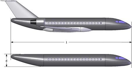
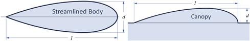
A streamlined body usually refers to a body-of-revolution, whose cross-section is similar to what is shown in Figure 15-34. A streamlined body is used to represent many types of fuselages, but also the hulls of airships. They can also be used to represent engine nacelles in drag estimation. A canopy refers to the external shape of an airplane’s glass helmet and is sized geometrically as shown in Figure 15-34. For more realistic canopies, refer to Section 15.5.10, Drag of canopies.
Fuselage as a Body of Revolution
In the following expressions, the fineness ratio, appropriately denoted by the letter f, is used to indicate the slenderness of a body of revolution. It is defined as follows:
![]() (15-67)
(15-67)
where l = length of the body and d = diameter of the body.
Although devised for bodies of revolution, the expressions for the form factors below are also applicable to bodies that are not truly ones of revolution, but feature cross-sectional shapes other than circular (see Figure 15-35). For instance, a cross-section might have the shape of a silhouette of an egg, or be box-shaped, or rectangular with round corners. These are treated by determining the shape’s maximum cross-sectional area, Amax, and then relating it to that of a circular cross-section using a “representative” fineness ratio as shown below:
![]() (15-68)
(15-68)
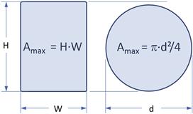
Form Factors at Subcritical Reynolds Numbers
Hoerner [3, p. 6-16] derives and suggests the following form factors for streamlined bodies at subcritical Reynolds numbers (Re < 105). The magnitude of the Re implies it could be the fuselages of small vehicles, such as radio-controlled aircraft, or small unmanned aerial vehicles. Note that since the expression includes the pressure drag component, it is not represented as a stand-alone form factor, but rather the product of the ![]() in Equation (15-59). It also requires the skin friction coefficient for laminar boundary layer of Equation (15-18) to be used:
in Equation (15-59). It also requires the skin friction coefficient for laminar boundary layer of Equation (15-18) to be used:
![]() (15-69)
(15-69)
Form Factors at Supercritical Reynolds Numbers
Hoerner [3, p. 6-17] suggests the following form factor for streamlined bodies in airflow whose Re > 105:
![]() (15-70)
(15-70)
Torenbeek [26] suggests the following form factor for a generic fuselage:
![]() (15-71)
(15-71)
Likewise, Nicolai [28] and Raymer [25] present the following form factor for a fuselage:
![]() (15-72)
(15-72)
Shevell [27, p. 179] also provides a model for a fuselage given by:
![]() (15-73)
(15-73)
Finally, Jenkinson’s model [29] is given by:
![]() (15-74)
(15-74)
where
Form Factor for Nacelle and Smooth External Store
Raymer [25] suggest the following form factors for nacelles:
![]() (15-75)
(15-75)
Jenkinson [29, p. 172] recommends simply using the constant FF·IF = 1.2 for wing mounted nacelles and FF·IF = 1.44 for nacelles mounted on the rear of the airplane (a Sud-Est Caravelle configuration).
Form Factors for Airship Hulls and Similar Geometries
If the fuselage closely resembles the hull of an airship (which, granted, most fuselages do not), then Equation (15-76), derived by Hoerner [3, p. 6-18] should be used.
![]() (15-76)
(15-76)
Note that it leads to substantially higher value of the form factor than do the other ones. However, it has a very distinct minimum around f ≈ 2.7.
A minimum fineness ratio of 2.7–3.5 for such bodies is well supported by experimental data and explains why fuselages of transport aircraft typically feature this fineness ratio for the aft end. A number of the above form factors are plotted in Figure 15-36.
EXAMPLE 15-6
Determine the minimum drag coefficient for the SR22, whose top view is shown in Figure 15-37, using the component drag build-up method. Note that the complete minimum drag coefficient is not just worked out here, but in a number of subsequent examples. The complete minimum drag coefficient is presented in Example 15-17.
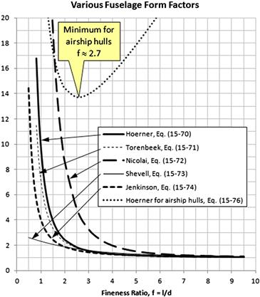
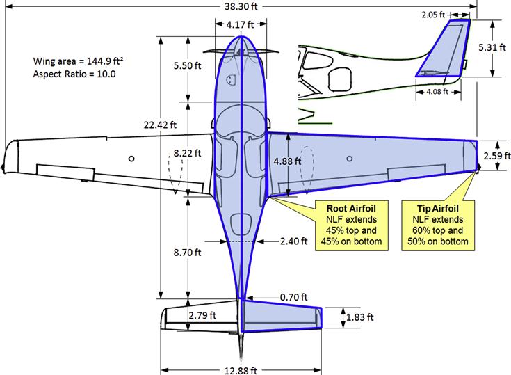
FIGURE 15-37 Geometry of the example aircraft showing the approximation of its wetted area. Note that for clarity some dimensions have been rounded off to two decimals.
Assume:
(1) Flight condition at S-L and 185 KTAS.
(2) Wing sustains laminar flow as detailed in Example 15-2.
(3) HT sustains 50% laminar flow on lower and upper surfaces.
(4) VT sustains 50% laminar flow on left and right surfaces.
(5) Fuselage sustains 5% laminar flow, cut short due to engine cowling assembly.
(6) Wetted area booster coefficient of 1.07 for wing and 1.05 for HT and VT.
(7) Max thickness for wing, HT, and VT is at 50% of the chord for all.
(8) t/c = 0.15 for wing, 0.1 for HT and VT, and 4.17/22.42 = 0.186 for the fuselage.
(9) Skin roughness value from Table (15-2).
(10) Assume the max thickness lines for the wing, HT, and VT to be 0°, 5°, and 18°, respectively.
(11) CDmisc is 6 drag counts and CDL&P is 3 drag counts.
(12) CRUD (see Section 15.5.1) is 25% of the sum of the above (×1.25).
Solution
The solution to this problem is relatively extensive due to the number of components that must be included. However, since many of the calculations are identical they are conveniently implemented in a spreadsheet as shown in Figure 15-38, Figure 15-39 and Figure 15-40. Each row has been numbered for convenience and sample calculations provided below for selected rows. The spreadsheet was designed to allow the user to enter geometry for other simple aircraft and determine the drag polar. Note that green cells are intended for user entry, whereas blue cells contain formulas.
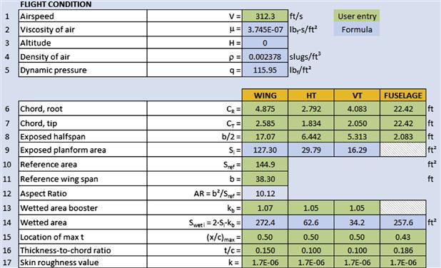

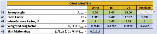
Begin by considering Figure 15-38, which shows cells with the given information (green cells) and five rows which show some calculation results (blue cells). Note the setup of the columns dedicated to the inboard and outboard wing elements, as well as the HT and VT.
Line 1: Airspeed is 185 KTAS × 1.688 ft/s per KTAS = 312.3 ft/s.
Line 2: Viscosity of air:
![]()
Lines 6-8, 10-13, and 15-17: Geometric data is obtained from Figure 15-37 and other data is entered based on the problem statement. Note that the exposed halfspan (and planform area) exclude the area of the surface that is inside the fuselage. Here it will be assumed that, of the components shown, only a part of the wing is inside the fuselage and this is reflected as the exposed halfspan and planform area.
Line 9: Exposed planform area.
Fuselage: not needed since a different method is used to determine its wetted area.
Line 14: Total wetted area of all components (entire exposed wing, HT, VT, and fuselage):
The total wetted area of the fuselage is estimated using the method of Section 12.4.3, Surface areas and volumes of a typical tubular fuselage, and the fuselage geometry of Figure 15-37, using Equation (12-13), repeated here for convenience:
![]() (12-13)
(12-13)
where
D = maximum fuselage diameter = 4.17 ft
L1 = length of nose section = 5.50 ft
Plugging and chugging those numbers into this equation yields 203 ft2. However, the author's own approximation, which accounts for more details in the fuselage and spinner geometry returned the following value.
Note that it would be prudent to subtract the cross-sectional area of the wing on the left and right sides, where it enters the fuselage, but in the interests of simplicity it is left out of these calculations. To calculate this cross-sectional area, the reader can for instance use the approximation of Section 9.2.4, Approximation of airfoil cross-sectional area. Now, let’s consider Figure 15-39, which shows the skin friction analysis for the root and tip chords.
Lines 18-19 and 28-29: Data entered is based on the problem statement.
Line 20: Reynolds number for the root chord (using the wing column as an example).
![]()
Lines 21-22 and 30-31: Here, the calculations for Lines 21-22 are used. The cutoff Reynolds number for the root chord (again using the wing column as an example) using Equation (15-25).
![]()
Since the Re based on CR is less than this value, it will be used throughout the remainder of these calculations. If the opposite had been the case, then the cutoff Re would been used.
Line 23-27 and 33-38: Steps 4 through 14 of Example 15-2 detail how the values for the wing column were obtained. All the values in the other three columns are calculated in an identical fashion, yielding the table shown in Line 42. Finally, consider Figure 15-40, which shows how the minimum drag coefficient is calculated.
Line 39: Thickness sweep angles for the wing, HT, and VT are given in the problem statement as 0°, 5°, and 18°, respectively.
Line 40: The form factor for the wing, HT, and VT are calculated using Equation (15-64) and Equation (15-72) for the fuselage. Note that 185 KTAS at sea level corresponds to M ≈ 0.28.
![]()
![]()
![]()
![]()
![]()
Where f is the fineness ratio, calculated from ![]()
Line 41: Interference factors are selected from Table 15-7.
Line 42: Weighted drag factor calculated as shown in table. For instance, for the wing we get;
![]()
Line 43: Skin friction drag is calculated by summing up the cells in Line 42 and dividing by the reference area of 144.9 ft2. The resulting total skin friction coefficient, which includes interference and form drag, is:
![]()
This only partially completes the drag analysis – drag due to miscellaneous sources remains to be determined and added to the above value, in addition to other corrections must be made. This will be done in the next section.
15.5 Miscellaneous or Additive Drag
In its most elementary form, the skin friction drag estimated using the component drag build-up method (CDBM) excludes drag caused by landing gear, antennas, sharp corners, joints, fasteners, inlets, outlets, fairings, and miscellaneous other protuberances all airplanes feature to some extent. This drag, which is justifiably referred to as miscellaneous or additive drag, must be accounted for as it increases the total drag well beyond what is predicted by CDBM. It is the purpose of this section to correct this deficiency by presenting a number of methods to account for it. As shown in Equation (15-59) this drag is treated using a special term, CDmisc. Thus, CDmisc is estimated as the sum of a number of contributing sources as shown below:
![]() (15-77)
(15-77)
where the series ΔCD1, ΔCD2, … are the contributions of all known components that add to the drag and were not accounted for using the CDBM (e.g. landing gear, antennas, etc.). Note that each contribution becomes an integral part of the minimum drag coefficient, CDmin. It, on the other hand, is used to calculate the total drag of the airplane using the reference wing area, Sref, as a primary variable. It follows that each contribution must be adjusted in terms of this reference area. Usually, the drag contributions are presented based on the geometry of the component itself, e.g. frontal area or side area or similar. This requires additional conversions to take place, as is explained below, to ensure it references Sref.
The geometric shape of protrusions typical to aircraft is inherently irregular. For instance, consider the dissimilar geometry of antennas, blisters, or the main landing gear typical of ordinary aircraft. None shares common dimensions like those shared by most lifting surfaces (e.g. wing, horizontal, and vertical tails). Each is geometrically complex enough to call for a drag estimation based on empirical formulation. This, in turn, means that the drag of the protrusion must be measured in a wind tunnel and then related to its own geometry and the Reynolds number at the test condition. Only then can it be applied to something as practical as aircraft design. The drag of such protrusions is frequently based on shape parameters, like the thickness-to-length ratio (or fineness ratio) of a particular component, or the location of is maximum thickness, or the frontal area, the lengthwise distribution of thickness, leading edge radius, trailing edge angle, and the camber, to name a few.
It is helpful to use descriptive subscripts when determining the drag coefficient of each such source. Thus, the drag coefficient of a specific antenna might be referred to as ΔCDantenna rather than, say, ΔCD7. The following sections assume such naming conventions. Now consider some geometric shape of interest whose drag force has been measured in a wind tunnel at a specific Reynolds number. Furthermore, assume this drag to be denoted by DS (where the subscript stands for source) and that, ultimately, we want the data to be applicable to an unrelated project. In order to accomplish this, the measurement must be converted into a drag coefficient, which here will be called ΔCDS. Furthermore, assume it references some geometry (typically some reference area other than the wing area) given by SS. Then, the drag coefficient of the component, ΔCDS, would be calculated from:
![]() (15-78)
(15-78)
However, as stated above, we want to refer this value to the reference wing area Sref and must thus scale the coefficient accordingly. We might refer to this scaled coefficient using the name of the source. For instance, the scaling of the aforementioned antenna, ΔCDantenna, would then be accomplished using the expression below:
![]() (15-79)
(15-79)
Derivation of Equation (15-79)
This expression is simply derived by noting the same value of the drag must be calculated regardless of whether one uses the source area or the reference area. Mathematically:
![]()
QED
15.5.1 Cumulative Result of Undesirable Drag (CRUD)
Of course the above title is just a play on words. The word crud means dirt, filth, or refuse. In aircraft design it stands for the undesirable drag caused by things like exhaust stacks, misaligned sheet-metal panels, antennas, small inlets and outlets, sanded walkways, and so on. These parts are easily overlooked when performing drag analysis, primarily because the evaluation of their contribution is next to impossible. For instance, consider misaligned sheet-metal panels for aluminum aircraft. The problem is not that there isn’t a method to estimate the drag of a misaligned panel, because there is, but rather that it is impossible to estimate how poorly or well the panels align until the actual aircraft is built. It is imperative the aspiring designer is aware of this drag and accounts for it appropriately. This section introduces how this is typically done.
In 1940 NACA released the wartime report WR-L-489 in which 11 military aircraft were investigated to determine why they didn’t meet predicted performance [30]. The report detailed wind tunnel testing of the aircraft in the NACA Full-Scale Wind Tunnel in Langley, Virginia. The aircraft were stripped to a clean configuration by gradually removing components and the drag coefficient was measured after each removal step. The results give a timeless insight into the cumulative impact of small and easily ignored design details on the total drag.
One of the aircraft investigated was the Seversky P-35 that had been designed for the US Army Air Corps in the early 1930s (see Figure 15-41). At the time, it was an innovative single-engine fighter that offered a number of firsts. It was the Air Corp’s first all-metal fighter, the first to feature a retractable landing gear, and the first with an enclosed cockpit. The P-35 had a predicted maximum airspeed in excess of 260 KTAS. However, in practice, it fell way short of that goal as the maximum airspeed was found to be some 20 KTAS less than that. While a part of the problem was that its engine could not develop the advertized power, this did not fully explain the large difference between practice and prediction. This simply implied its drag was higher than predicted – something common to other aircraft of the period as well. After all, that is why 11 aircraft, rather than a single one, were studied in the report. This highlights a scenario that anyone estimating the drag of a new airplane may find himself in – to assume the cleanliness of Airplane 1 in Figure 15-41, when in reality it will be closer to Airplane 18.
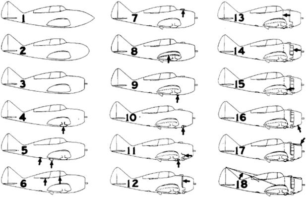
FIGURE 15-41 Order of modifications made to the Seversky P-35 aircraft during wind tunnel testing. Arrow points to the location of changes. Figure from NACA WR-L-489.
Such under-predictions are not limited to aircraft of the yesteryear. They still happen. A recently developed small twin-engine business jet was unable to meet the predicted performance advertised on the company website. This led to a costly redevelopment effort and eventually the airplane was shown to meet the promised capabilities. A small single-engine propeller aircraft developed by a prominent car manufacturer also didn’t meet the predicted performance, allegedly due to drag higher than predicted. Both aircraft were designed by people who cannot be accused of not knowing what they were doing. It shows that no matter one’s proficiency, under-prediction of drag is a likely scenario and the subject must be handled with utmost caution.
Going back to the NACA WR-L-489, the source presents a detailed listing of the changes made to the airplane presented in a graphic and tabulates their effect on the total drag. The graphic is reproduced as Figure 15-41 and the table is recreated as Table 15-8. It should be of great interest to the aircraft designer to inspect the table and consider how the contributions of seemingly insignificant modifications, such as a sanded walkway or an opened cowl flap, affect the overall drag of the airplane. The problem is not the value of individual component, but rather their cumulative effect.

15.5.2 Trim Drag
Trim drag is the penalty paid for providing static stability. Technically, trim drag is the combination of two sources.
(1) The difference in lift-induced drag of the airplane with and without balancing forces and (2) the increase in drag due to the deflection of the elevator (see Section 15.4.4, The Effect of Control Surface Deflection –Trim Drag). This is denoted using the variable ![]() . Its value typically ranges from 0.0000 to 0.0005 per degree of elevator deflection. It must be multiplied by the elevator deflection to trim, δe, to determine the additive drag coefficient.
. Its value typically ranges from 0.0000 to 0.0005 per degree of elevator deflection. It must be multiplied by the elevator deflection to trim, δe, to determine the additive drag coefficient.
If a longitudinally stable airplane could sustain steady level flight without having to generate a balancing force there would be no trim drag. The balancing force of a statically stable conventional tail-aft aircraft is added to the weight. This implies the total lift generated by the wing must be greater than the weight alone. This requires it to operate at a higher AOA and, thus, at a higher lift-induced drag than otherwise. It does not matter whether this stability is generated using a horizontal tail, such as that of the statically stable tail-aft configuration, or using airfoils and elevons, such as that of a flying wing; the total drag of the airplane is increased. This section presents a method to estimate the trim drag.
Since trim drag is a consequence of the longitudinal stability, it is easy to derive a complicated and unwieldy formulation that is of limited practical use. Ordinarily, trim drag constitutes a small fraction of the total drag of the airplane; it should range from 1% to 2%. During the design process, it is more practical to estimate the trim drag using a simple formulation and this is what will be demonstrated here. The same methodology can be revised to account for more complex situations. Note that the method assumes the airplane is operating at a low AOA, allowing for simplification.
Trim Drag of a Simple Wing-Horizontal Tail Combination
Consider the simple wing-HT system shown in Figure 15-42. Note the equation is presented in a form that lends itself well when considering changes in the location of the CG. For this system the trim drag is given by:
![]() (15-80)
(15-80)
where
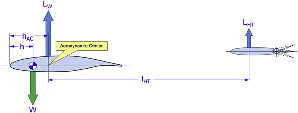
Derivation of Equation (15-80)
Referring to Figure 15-42, statics requires the following to hold in steady level flight:
![]()
These can be solved for the balancing force the HT must generate:
![]()
Inserting this result into the force equation leads to: