More than most other systems management processes, storage management involves a certain degree of trust. Users entrust us with the safekeeping of their data. They trust that they will be able to access their data reliably in acceptable periods of time. They trust that, when they retrieve it, it will be in the same state and condition as it was when they last stored it. Infrastructure managers trust that the devices they purchase from storage-equipment suppliers will perform reliably and responsively; suppliers, in turn, trust that their clients will operate and maintain their equipment properly.

We will interweave this idea of trust into our discussion on the process of managing data storage. The focus will be on four major areas:

Recoverability plays a fundamental role in disaster recovery. Many an infrastructure has felt the impact of not being able to recover yesterday’s data. How thoroughly we plan and manage storage in anticipation of tomorrow’s disaster may well determine our success in recovery.

We begin with a formal definition of the storage management process and a discussion of desirable traits in a process owner. We then examine each of the four storage management areas in greater detail and reinforce our discussion with examples where appropriate. We conclude this chapter with assessment worksheets for evaluating an infrastructure’s storage management process.

Optimizing the use of storage devices translates into making sure the maximum amount of usable data is written to and read from these units at an acceptable rate of response. Optimizing these resources also means ensuring that there is an adequate amount of storage space available while guarding against having expensive excess amounts. This notion of optimal use ties in to two of the main areas of storage management: capacity and performance.

Protecting the integrity of data means that the data will always be accessible to those authorized to it and that it will not be changed unless the authorized owner specifically intends for it to be changed. Data integrity also implies that, should the data inadvertently become inaccessible or destroyed, reliable backup copies will enable its complete recovery. These explanations of data integrity tie into the other two main areas of storage management: reliability and recoverability. Each of these four areas warrants a section of its own, but first we need to discuss the issue of process ownership.

The individual who is assigned as the owner of the storage management process should have a broad basis of knowledge in several areas related to disk space resources. These areas include applications, backup systems, hardware configurations, and database systems. Due to the dynamic nature of disk-space management, the process owner should also be able to think and act in a tactical manner. Table 12-1 lists, in priority order, these and other desirable characteristics to look for when selecting this individual.

Another issue to keep in mind when considering candidates for storage management process owner is that the individual’s traits may also make him or her a candidate to own other related processes—the person may already be a process owner of another process. The following four primary areas of storage management are directly related to other systems management processes:

The storage management process owner may be qualified to own one or more of these other processes, just as an existing owner of any of these other processes might be suitable to own storage management. In most instances, these process owners report to the manager of technical services, if they are not currently serving in that position themselves.

Storage management capacity consists of providing sufficient data storage to authorized users at a reasonable cost. Storage capacity is often thought of as large quantities of disk farms accessible to servers or mainframes. In fact, data storage capacity includes main memory and magnetic disk storage for mainframe processors, midrange computers, workstations, servers, and desktop computers in all their various flavors. Data storage capacity also includes alternative storage devices such as optical disks, magnetic drums, open reel magnetic tape, magnetic tape cartridges and cassettes, digital audio tape, and digital linear tape. When it comes to maximizing the efficient use of data storage, most efforts are centered around large-capacity storage devices such as high-volume disk arrays. This is because the large capacities of these devices, when left unchecked, can result in poorly used or wasted space.

There are a number of methods to increase the utilization of large-capacity storage devices. One is to institute a robust capacity planning process across all of IT that will identify far in advance major disk space requirements. This enables planners to propose and budget the most cost-effective storage resources to meet forecast demand. Another more tactical initiative is to monitor disk space usage to proactively spot unplanned data growth, data fragmentation, increased use of extents, and data that has not been accessed for long periods of time. There are a number of tools on the market that can streamline much of this monitoring. The important element here is the process, rather than the tool, that needs to be enforced to heighten awareness about responsible disk space management.

The advent of the personal computer in the 1970s brought with it the refinement of portable disk storage (see Table 12-2) beginning with the diskette or so-called floppy disk. Early versions were 8 inches wide, stored 80 kilobytes of data, and recorded only on one side. Refinements eventually reduced its size to 3.5 inches (see Figure 12-1) and increased its capacity to 1.44 megabytes. By 2001, both Sony Corporation and Phillips Electronics had refined and offered to consumers the universal serial bus (USB) flash drive. These devices were non-volatile (they retained data in absence of power), solid state, and used flash memory. More importantly, they consumed only 5 percent of the power of a small disk drive, were tiny in size, and were very portable. Users have come to know these devices by various names, including:

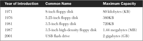
Figure 12-1. 3.5-Inch Floppy Disk “Reprint courtesy of International Business Machines Corporation, copyright International Business Machines Corporation”

Regardless of what they are called, they have proven to be very reliable and very popular.

While magnetic disks are the most common type of storage device within an infrastructure, magnetic tape is still an important part of this environment. Huge databases and data warehouses now command much of the attention of storage managers, but all this data is still primarily backed-up to tape. Just as disk technology has advanced, the increased data capacities of tape have also evolved significantly over the past few decades (see Table 12-3).

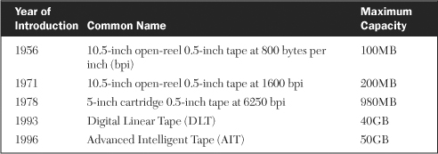
During the 1970s, nine-track magnetic tape density on a 10 1/2-inch open-reel increased from 800 bytes per inch (bpi) to 1,600 bpi, which was a capacity increase from 100 megabytes (MB) to 200MB. Toward the end of that decade, the number of tracks per tape and bytes per track both doubled, increasing the density to 6,250 bpi and the capacity to nearly a gigabyte. Subsequent advances into high density tapes doubled and tripled those capacities during the 1980s. The next technology to be developed in this arena was Digital Linear Tape (DLT), which has a unique helixical bit-pattern striping that results in 30 to 40 gigabytes (GB) per tape (see Figure 12-2). A few years later Sony pioneered Advanced Intelligent Tape (AIT). AIT can store over 50GBper tape and transfer data at six MB per second. Knowledge of these high-density tapes and their cost is important for storage management process owners who have to plan for backup windows, estimated restore times, and onsite and offsite floor space for housing these tapes.

Figure 12-2. Digital Linear Tape (DLT)

There are a variety of considerations that come into play when configuring infrastructure storage for optimal performance. The following list shows some of the most common of these. We will start with performance considerations at the processor side and work our way out to the storage devices.

1. Size and type of processor main memory
2. Number and size of buffers
3. Size of swap space
4. Number and type of channels
5. Device controller configuration
6. Logical volume groups
7. Amount of disk array cache memory
8. Storage area networks (SANs)
9. Network-attached storage (NAS)

The first performance consideration is the size and type of main memory. Processors of all kinds—from desktops up to mainframes—have their performance impacted by the amount of main storage installed in them. The amount can vary from just a few megabytes for desktops to up to tens of gigabytes for mainframes. Computer chip configurations, particularly for servers, also vary from 128MB to 256MB to forthcoming 1GB memory chips. The density can influence the total amount of memory that can be installed in a server due to the limitation of physical memory slots.

In smaller shops, systems administrators responsible for server software may also configure and manage main storage. In larger shops, disk storage analysts likely interact with systems administrators to configure the entire storage environment, including main memory, for optimal performance. These two groups of analysts also normally confer about buffers, swap space, and channels. The number and size of buffers are calculated to maximize data-transfer rates between host processors and external disk units without wasting valuable storage and cycles within the processor. Similarly, swap space is sized to minimize processing time by providing the proper ratio of real memory space to disk space. A good rule of thumb for this ratio used to be to size the swap space to be equal to that of main memory, but today this will vary depending on applications and platforms.

Channels connecting host processors to disk and tape storage devices vary as to their transfer speed, their technology, and the maximum number able to be attached to different platforms. The number and speed of the channels influence performance, response, throughput, and costs. All of these factors should be considered by storage management specialists when designing an infrastructure’s channel configurations.

Tape and disk controllers have variable numbers of input channels attaching them to their host processors, as well as variable numbers of devices attaching to their output ports. Analysis needs to be done to determine the correct number of input channels and output devices per controller to maximize performance while still staying within reasonable costs. There are several software analysis tools available to assist in this; often the hardware suppliers can offer the greatest assistance.

A software methodology called a logical volume group assembles together two or more physical disk volumes into one logical grouping for performance reasons. This is most commonly done on huge disk-array units housing large databases or data warehouses. The mapping of physical units into logical groupings is an important task that almost always warrants the assistance of performance specialists from the hardware supplier or other sources.

To improve performance of disk transactions, huge disk arrays also have varying sizes of cache memory. Large database applications benefit most from utilizing a very fast—and very expensive—high-speed cache. Because of the expense of the cache, disk-storage specialists endeavor to tune the databases and the applications to make maximum use of the cache. Their goal is to have the most frequently accessed parts of the database residing in the cache. Sophisticated pre-fetch algorithms determine which data is likely to be requested next and then initiate the preloading of it into the cache. The effectiveness of these algorithms greatly influences the speed and performance of the cache. Since the cache is read first for all disk transactions, finding the desired piece of data in the cache—for example, a hit—greatly improves response times by eliminating the relatively slow data transfer from physical disks. Hit ratios (hits versus misses) between 85 percent and 95 percent are not uncommon for well-tuned databases and applications; this high hit ratio helps justify the cost of the cache.

Two more recent developments in configuring storage systems for optimal performance are storage area networks (SANs) and network attached storage (NAS). SAN is a configuration enhancement that places a high-speed fiber-optic switch between servers and disk arrays. The two primary advantages are speed and flexibility. NAS is similar in concept to SAN except that the switch in NAS is replaced by a network. This enables data to be shared between storage devices and processors across a network. There is a more detailed discussion on the performance aspects of these two storage configurations described in Chapter 8, “Performance and Tuning.”

Robust storage management implies that adequate amounts of disk storage are available to users whenever they need it and wherever they are. However, the reliability of disk equipment has always been a major concern of hardware suppliers and customers alike. This emphasis on reliability can be illustrated with a highly publicized anecdote involving IBM that occurred almost 30 years ago.

IBM had always been proud that it had never missed a first customer ship date for any major product in the company’s history. In late 1980, it announced an advanced new disk drive (the model 3380) with a first customer ship date of October 1981. Anticipation was high because this model would have tightly packed tracks with densely packed data, providing record storage capacity at an affordable price.

While performing final lab testing in the summer of 1981, engineers discovered that, under extremely rare conditions, the redundant power supply in the new model drive could intermittently malfunction. If another set of conditions occurred at the same time, a possible write error could result. A team of engineering specialists studied the problem for weeks but could not consistently duplicate the problem, which was necessary to enable a permanent fix. A hotly contested debate ensued within IBM about whether the should delay shipment until the problem could be satisfactorily resolved, with each side believing that the opposing position would do irreparable damage to the corporation.

The decision went to the highest levels of IBM management, who decided they could not undermine the quality of their product or jeopardize the reputation of their company by adhering to an artificial schedule with a suspect offering. In August, IBM announced it was delaying general availability of its model 3380 disk drive system for at least three months, perhaps even longer if necessary. Wall Street, industry analysts, and interested observers held their collective breath, expecting major fallout from the announcement. It never came. Customers were more impressed than disappointed by IBM’s acknowledgment of the criticality of disk drive reliability. Within a few months the problem was traced to a power supply filter that was unable to handle rare voltage fluctuations. It was estimated at the time that the typical shop using clean, or conditioned, power had less than a one-in-a-million chance of ever experiencing the set of conditions required to trigger the malfunction.

The episode served to strengthen the notion of just how important reliable disk equipment was becoming. With companies beginning to run huge corporate databases on which the success of their business often depended, data storage reliability was of prime concern. Manufacturers began designing into their disk storage systems redundant components such as backup power systems, dual channel ports to disk controllers, and dual pathing between drives and controllers. These improvements significantly increased the reliability of disk and tape storage equipment, in some instances more than doubling the usual one-year mean time between failures (MTBF) for a disk drive. Even with this improved reliability, the drives were far from fault tolerant. If a shop had 100 disk drives—not uncommon at that time—it could expect an average failure rate of one disk drive per week.

Fault-tolerant systems began appearing in the 1980s, a decade in which entire processing environments were duplicated in a hot standby mode. These systems essentially never went down, making their high cost justifiable for many manufacturing companies with large, 24-hour workforces, who needed processing capability but not much in the way of databases. Most of the cost was in the processing part since databases were relatively small and disk storage requirements were low. However, there were other types of companies that had large corporate databases requiring large amounts of disk storage. The expense of duplicating huge disk farms all but put most of them out of the running for fault-tolerant systems.

During this time, technological advances in design and manufacturing drove down the expense of storing data on magnetic devices. By the mid-1980s, the cost per megabyte of disk storage had plummeted to a fraction of what it had been a decade earlier. Smaller, less reliable disks such as those on PCs were less expensive still. But building fault-tolerant disk drives was still an expensive proposition due to the complex software needed to run high-capacity disks in a hot standby mode in concert with the operating system. Manufacturers then started looking at connecting huge arrays of small, slightly less reliable and far less expensive disk drives and operating them in a fault-tolerant mode that was basically independent of the operating systems on which they ran. This was accomplished by running a separate drive in the array for parity bits.

This type of disk configuration was called a redundant array of inexpensive disks (RAID). By the early 1990s, most disk drives were considered inexpensive, moving the RAID Advisory Board to officially change the I in RAID to independent rather than inexpensive. Advances and refinements led to improvements in affordability, performance, and especially reliability. Performance was improved by disk striping, which writes data across multiple drives, increasing data paths and transfer rates and allowing simultaneous reading and writing to multiple disks. This implementation of RAID is referred to as level 0. Reliability was improved through mirroring (level 1) or use of parity drives (level 3 or 5). The result is that RAID has become the de facto standard for providing highly reliable disk-storage systems to mainframe, midrange, and client/server platforms. Table 12-4 lists the five most common levels of RAID.

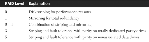
Mirroring at RAID level 1 means that all data is duplicated on separate drives so that if one drive malfunctions, its mirrored drive maintains uninterrupted operation of all read and write transactions. Software and microcode in the RAID controller take the failing drive offline and issue messages to appropriate personnel to replace the drive while the array is up and running. More sophisticated arrays notify a remote repair center and arrange replacement of the drive with the supplier with little or no involvement of infrastructure personnel. This level offers virtually continuous operation of all disks.

The combination of striping and mirroring goes by several nomenclatures, including:

As its various names suggest, this level of RAID duplicates all data for high reliability and stripes the data for high performance.

RAID level 3 stripes the data for performance reasons similar to RAID level 0 and, for high reliability, assigns a dedicated parity drive on which parity bits are written to recover and rebuild data in the event of a data drive malfunction. There are usually two to four data drives supported by a single parity drive.

RAID level 5 is similar to level 3 except that parity bits are shared on nonassociated data drives. For example, for three data drives labeled A, B, and C, the parity bits for data striped across drives B and C would reside on drive A; the parity bits for data striped across drives A and C would reside on drive B; the parity bits for data striped across drives A and B would reside on drive C.

A general knowledge about how an application accesses data can help in determining which level of RAID to employ. For example, the relatively random access into the indexes and data files of a relational database make them ideal candidates for RAID 0+1. The sequential nature of log files would make them better candidates for just RAID 1 alone. By understanding the different RAID levels, storage management process owners can better evaluate which scheme is best suited for their business goals, their budgetary targets, their expected service levels, and their technical requirements.

There are several methods available for recovering data that has been altered, deleted, damaged, or otherwise made inaccessible. Determining the correct recovery technique depends on the manner in which the data was backed up. Table 12-5 lists four common types of data backups. The first three are referred to as physical backups because operating system software or specialized program products copy the data as it physically resides on the disk without regard to database structures or logical organization—it is purely a physical backup. The fourth is called a logical backup because database management software reads—or backs up—logical parts of the database, such as tables, schemas, data dictionaries, or indexes; the software then writes the output to binary files. This may be done for the full database, for individual users, or for specific tables.

Physical offline backups require shut down of all online systems, applications, and databases residing on the volume being backed up prior to starting the backup process. Performing several full volume backups of high-capacity disk drives may take many hours to complete and are normally done on weekends when systems can be shut down for long periods of time. Incremental backups also require systems and databases to be shut down, but for much shorter periods of time. Since only the data that has changed since the last backup is what is copied, incremental backups can usually be completed within a few hours if done on a nightly basis.

A physical online backup is a powerful backup technique that offers two very valuable and distinct benefits:

The database environment must be running in an archive mode for online backups to occur properly. This means that fully filled log files, prior to being written over, are first written to an archive file. During online backups, table files are put into a backup state one at a time to enable the operating system to back up the data associated with it. Any changes made during the backup process are temporarily stored in log files and then brought back to their normal state after that particular table file has been backed up.

Full recovery is accomplished by restoring the last full backup and the incremental backups taken since the last full backup and then doing a forward recovery utilizing the archive and log tapes. For Oracle databases, the logging is referred to as redo files; when these files are full, they are copied to archive files before being written over for continuous logging. Sybase, IBM’s Database 2 (DB2), and Microsoft’s SQL Server have similar logging mechanisms using checkpoints and transaction logs.

Logical backups are less complicated and more time consuming to perform. There are three advantages to performing logical backups in concert with physical backups:

1. Exports can be made online, enabling 24/7 applications and databases to remain operational during the copying process.
2. Small portions of a database can be exported and imported, efficiently enabling maintenance to be performed on only the data required.
3. Exported data can be imported into databases or schemas at a higher version level than the original database, allowing for testing at new software levels.

Another approach to safeguarding data becoming more prevalent today is the disk-to-disk backup. As the size of critical databases continues to grow, and as allowable backup windows continue to shrink, there are a number of advantages to this approach that help to justify its obvious costs. Among these advantages are:

A thorough understanding of the requirements and the capabilities of data backups, restores, and recovery is necessary for implementing a robust storage management process. Several other backup considerations need to be kept in mind when designing such a process. They are as follows:

1. Backup window
2. Restore times
3. Expiration dates
4. Retention periods
5. Recycle periods
6. Generation data groups
7. Offsite retrieval times
8. Tape density
9. Tape format
10. Tape packaging
11. Shelf life
12. Automation techniques

There are three key questions that need to be answered at the outset:

1. How much nightly backup window is available?
2. How long will it take to perform nightly backups?
3. Back to what point in time should recovery be made?

If the time needed to back up all the required data on a nightly basis exceeds the offline backup window, then some form of online backup will be necessary. The method of recovery used depends on whether data will be restored back to the last incremental backup or back to the last transaction completed.

Expiration dates, retention periods, and recycling periods are related issues pertaining to the length of time data is intended to stay in existence. Weekly and monthly application jobs may create temporary data files that are designed to expire one week or one month, respectively, after the data was generated. Other files may need to be retained for several years for auditing purposes or for government regulations. Backup files on tape also fall into these categories. Expiration dates and retention periods are specified in the job-control language that describes how these various files will be created. Recycle periods relate to the elapsed time before backup tapes are reused.

A generation data group (GDG) is a mainframe mechanism for creating new versions of a data file that would be similar to that created with backup jobs. The advantage of this is the ability to restore back to a specific day with simple parameter changes to the job-control language. Offsite retrieval time is the maximum contracted time that the offsite tape storage provider is allowed to physically bring tapes to the data center from the time of notification.

Tape density, format, and packaging relate to characteristics that may change over time and consequently change recovery procedures. Density refers to the compression of bits as they are stored on the tape; it will increase as technology advances and equipment is upgraded. Format refers to the number and configuration of tracks on the tape. Packaging refers to the size and shape of the enclosures used to house the tapes.

The shelf life of magnetic tape is sometimes overlooked and can become problematic for tapes with retention periods exceeding five or six years. Temperature, humidity, handling, frequent changes in the environment, the quality of the tape, and other factors can influence the actual shelf life of any given tape, but five years is a good rule of thumb to use for recopying long-retained tapes.

Mechanical tape loaders, automated tape library systems, and movable tape rack systems can all add a degree of labor-saving automation to the storage management process. As with any process automation, thorough planning and process streamlining must precede the implementation of the automation.

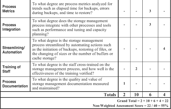
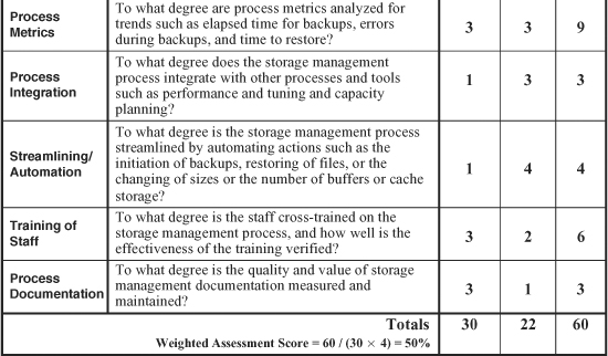
The worksheets shown in Figures 12-3 and 12-4 present a quick-and-simple method for assessing the overall quality, efficiency, and effectiveness of a storage management process. The first worksheet is used without weighting factors, meaning that all 10 categories are weighted evenly for the assessment of a storage management process. Sample ratings are inserted to illustrate the use of the worksheet. In this case, the storage management process scored a total of 22 points for an overall nonweighted assessment score of 55 percent. The second sample (weighted) worksheet compiled a weighted assessment score of 50 percent.

One of the most valuable characteristics of these worksheets is that they are customized to evaluate each of the 12 processes individually. The worksheets in this chapter apply only to the storage management process. However, the fundamental concepts applied in using these evaluation worksheets are the same for all 12 disciplines. As a result, the detailed explanation on the general use of these worksheets presented near the end of Chapter 7, “Availability,” also applies to the other worksheets in the book. Please refer to that discussion if you need more information.

We can measure and streamline the storage management process with the help of the assessment worksheet shown in Figure 12-3. We can measure the effectiveness of a storage management process with service metrics such as outages caused by either lack of disk space or disk hardware problems and poor response due to fragmentation or lack of reorganizations. Process metrics—such as elapsed time for backups, errors during backups, and time to restore—help us gauge the efficiency of this process. And we can streamline the storage management process by automating actions such as the initiation of backups, restoring of files, or the changing of sizes or the number of buffers or cache storage.

This chapter discussed the four major areas of the storage management process: capacity, performance, reliability, and recoverability. We began in our usual manner with a definition for this process and desirable characteristics in a process owner. We then presented key information about each of the four major areas.

We looked at techniques to manage storage capacity from both a strategic and tactical standpoint. A number of performance considerations were offered to optimize overall data-transfer rates in large-capacity storage arrays. We next discussed reliability and recoverability. These are companion topics relating to data integrity, which is the most significant issue in the process of storage management.

The discussion on reliability included an industry example of its importance and how RAID evolved into a very effective reliability feature. A number of considerations for managing backups were included in the discussion on recoverability. The customized assessment sheets were provided to evaluate an infrastructure’s storage management process.

1. For disk controllers with cache memory, the lower the hit ratio, the better the performance. (True or False)
2. A physical backup takes into account the structures and logical organization of a database. (True or False)
3. Which of the following is not an advantage of a disk-to-disk backup?

   a. significantly reduces backup and recovery time

   b. is less expensive than a disk-to-tape backup

   c. helps facilitate data replication

   d. the stored copy can be used for other purposes

4. The type of backup that uses database management software to read and copy parts of a database is called a ___________ _____________ .
5. Describe some of the advantages and disadvantages of storage capacities becoming larger and denser.

1. http://cs-exhibitions.uni-klu.ac.at/index.php?id=310
2. Storage Area Networks for Dummies; 2003; Poelker, Christopher and Nikitin, Alex; For Dummies Publishing
3. www.bitpipe.com/tlist/Data-Replication.html
4. Using SANs and NAS; 2002; Preston, Curtis; O’Reilly Media
5. www.emc.com/products/systems/DMX_series.jsp