CHAPTER 7
FINANCIAL ANALYSIS TECHNIQUES
After completing this chapter, you will be able to do the following:
- Describe tools and techniques used in financial analysis, including their uses and limitations.
- Classify, calculate, and interpret activity, liquidity, solvency, profitability, and valuation ratios.
- Describe the relationships among ratios and evaluate a company using ratio analysis.
- Demonstrate the application of DuPont analysis of return on equity, and calculate and interpret the effects of changes in its components.
- Calculate and interpret ratios used in equity analysis, credit analysis, and segment analysis.
- Describe how ratio analysis and other techniques can be used to model and forecast earnings.
Financial analysis tools can be useful in assessing a company’s performance and trends in that performance. In essence, an analyst converts data into financial metrics that assist in decision making. Analysts seek to answer such questions as: How successfully has the company performed, relative to its own past performance and relative to its competitors? How is the company likely to perform in the future? Based on expectations about future performance, what is the value of this company or the securities it issues?
A primary source of data is a company’s annual report, including the financial statements and notes, and management commentary (operating and financial review or management’s discussion and analysis). This chapter focuses on data presented in financial reports prepared under International Financial Reporting Standards (IFRS) and United States generally accepted accounting principles (U.S. GAAP). However, financial reports do not contain all the information needed to perform effective financial analysis. Although financial statements do contain data about the past performance of a company (its income and cash flows) as well as its current financial condition (assets, liabilities, and owners’ equity), such statements do not necessarily provide all the information useful for analysis nor do they forecast future results. The financial analyst must be capable of using financial statements in conjunction with other information to make projections and reach valid conclusions. Accordingly, an analyst typically needs to supplement the information found in a company’s financial reports with other information, including information on the economy, industry, comparable companies, and the company itself.
This chapter describes various techniques used to analyze a company’s financial statements. Financial analysis of a company may be performed for a variety of reasons, such as valuing equity securities, assessing credit risk, conducting due diligence related to an acquisition, or assessing a subsidiary’s performance. This chapter will describe techniques common to any financial analysis and then discuss more specific aspects for the two most common categories: equity analysis and credit analysis.
Equity analysis incorporates an owner’s perspective, either for valuation or performance evaluation. Credit analysis incorporates a creditor’s (such as a banker or bondholder) perspective. In either case, there is a need to gather and analyze information to make a decision (ownership or credit); the focus of analysis varies because of the differing interest of owners and creditors. Both equity and credit analyses assess the entity’s ability to generate and grow earnings, and cash flow, as well as any associated risks. Equity analysis usually places a greater emphasis on growth, whereas credit analysis usually places a greater emphasis on risks. The difference in emphasis reflects the different fundamentals of these types of investments: The value of a company’s equity generally increases as the company’s earnings and cash flow increase, whereas the value of a company’s debt has an upper limit.1
The balance of this chapter is organized as follows: Section 2 recaps the framework for financial statements and the place of financial analysis techniques within the framework. Section 3 provides a description of analytical tools and techniques. Section 4 explains how to compute, analyze, and interpret common financial ratios. Sections 5 through 8 explain the use of ratios and other analytical data in equity analysis, credit analysis, segment analysis, and forecasting, respectively. Section 9 summarizes the key points of the chapter, and practice problems in the CFA Institute multiple-choice format conclude the chapter.
2. THE FINANCIAL ANALYSIS PROCESS
In financial analysis, it is essential to clearly identify and understand the final objective and the steps required to reach that objective. In addition, the analyst needs to know where to find relevant data, how to process and analyze the data (in other words, know the typical questions to address when interpreting data), and how to communicate the analysis and conclusions.
2.1. The Objectives of the Financial Analysis Process
Because of the variety of reasons for performing financial analysis, the numerous available techniques, and the often-substantial amount of data, it is important that the analytical approach be tailored to the specific situation. Prior to beginning any financial analysis, the analyst should clarify the purpose and context, and clearly understand the following:
- What is the purpose of the analysis? What questions will this analysis answer?
- What level of detail will be needed to accomplish this purpose?
- What data are available for the analysis?
- What are the factors or relationships that will influence the analysis?
- What are the analytical limitations, and will these limitations potentially impair the analysis?
Having clarified the purpose and context of the analysis, the analyst can select the set of techniques (e.g., ratios) that will best assist in making a decision. Although there is no single approach to structuring the analysis process, a general framework is set forth in Exhibit 7-1.2 The steps in this process were discussed in more detail in an earlier chapter; the primary focus of this chapter is on Phases 3 and 4, processing and analyzing data.
EXHIBIT 7-1 A Financial Statement Analysis Framework
| Phase | Sources of Information | Output |
| 1. Articulate the purpose and context of the analysis |
|
|
| 2. Collect input data |
|
|
| 3. Process data |
|
|
| 4. Analyze/interpret the processed data |
|
|
| 5. Develop and communicate conclusions and recommendations (e.g., with an analysis report) |
|
|
| 6. Follow up |
|
|
2.2. Distinguishing between Computations and Analysis
An effective analysis encompasses both computations and interpretations. A well-reasoned analysis differs from a mere compilation of various pieces of information, computations, tables, and graphs by integrating the data collected into a cohesive whole. Analysis of past performance, for example, should address not only what happened but also why it happened and whether it advanced the company’s strategy. Some of the key questions to address include:
- What aspects of performance are critical for this company to successfully compete in this industry?
- How well did the company’s performance meet these critical aspects? (Established through computation and comparison with appropriate benchmarks, such as the company’s own historical performance or competitors’ performance.)
- What were the key causes of this performance, and how does this performance reflect the company’s strategy? (Established through analysis.)
If the analysis is forward looking, additional questions include:
- What is the likely impact of an event or trend? (Established through interpretation of analysis.)
- What is the likely response of management to this trend? (Established through evaluation of quality of management and corporate governance.)
- What is the likely impact of trends in the company, industry, and economy on future cash flows? (Established through assessment of corporate strategy and through forecasts.)
- What are the recommendations of the analyst? (Established through interpretation and forecasting of results of analysis.)
- What risks should be highlighted? (Established by an evaluation of major uncertainties in the forecast and in the environment within which the company operates.)
Example 7-1 demonstrates how a company’s financial data can be analyzed in the context of its business strategy and changes in that strategy. An analyst must be able to understand the “why” behind the numbers and ratios, not just what the numbers and ratios are.
EXAMPLE 7-1 Strategy Reflected in Financial Performance
Apple Inc. (NasdaqGS: AAPL) and Dell Inc. (NasdaqGS: DELL) engage in the design, manufacture, and sale of computer hardware and related products and services. Selected financial data for 2007 through 2009 for these two competitors follow here. Apple’s fiscal year (FY) ends on the final Saturday in September (for example, FY2009 ended on 26 September 2009). Dell’s fiscal year ends on the Friday nearest 31 January (for example, FY2009 ended on 29 January 2010 and FY2007 ended on 1 February 2008).
Source: Apple’s Forms 10-K and 10-K/A and Dell’s Form 10-K.
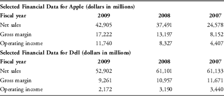
Apple reported a 53 percent increase in net sales from FY2007 to FY2008 and a further increase in FY2009 of approximately 14 percent. Gross margin increased 62 percent from FY2007 to FY2008 and increased 30 percent from FY2008 to FY2009. From FY2007 to FY2009, the gross margin more than doubled. Also, the company’s operating income almost tripled over the three-year period. From FY2007 to 2009, Dell reported a decrease in sales, gross margin, and operating income.
What caused Apple’s dramatic growth in sales and operating income and Dell’s comparatively sluggish performance? One of the most important factors was the introduction of innovative and stylish products, the linkages with iTunes, and expansion of the distinctive Apple stores. Among the company’s most important and most successful new products was the iPhone. Apple’s 2009 10-K indicates that iPhone unit sales grew 78 percent from 11.6 million units in 2008 to 20.7 million units in 2009. By 2009, the company’s revenues from iPhones and related services had grown to $13.0 billion and were nearly as large as the company’s $13.8 billion revenues from sales of Mac computers. The new products and linkages among the products not only increased demand but also increased the potential for higher pricing. As a result, gross profit margins and operating profit margins increased over the period because costs did not increase at the same pace as sales. Moreover, the company’s products revolutionized the delivery channel for music and video. The financial results reflect a successful execution of the company’s strategy to deliver integrated, innovative products by controlling the design and development of both hardware and software.
Dell continued to concentrate in the personal computer market, which arguably is in the market maturity stage of the product life cycle. Dell’s results are consistent with a market maturity stage where industry sales level off and competition increases so that industry profits decline. With increased competition, some companies cannot compete and drop out of the market.
Analysts often need to communicate the findings of their analysis in a written report. Their reports should communicate how conclusions were reached and why recommendations were made. For example, a report might present the following:3
- The purpose of the report, unless it is readily apparent.
- Relevant aspects of the business context:
- Economic environment (country, macro economy, sector).
- Financial and other infrastructure (accounting, auditing, rating agencies).
- Legal and regulatory environment (and any other material limitations on the company being analyzed).
- Evaluation of corporate governance and assessment of management strategy, including the company’s competitive advantage(s).
- Assessment of financial and operational data, including key assumptions in the analysis.
- Conclusions and recommendations, including limitations of the analysis and risks.
An effective narrative and well supported conclusions and recommendations are normally enhanced by using 3–10 years of data, as well as analytic techniques appropriate to the purpose of the report.
3. ANALYTICAL TOOLS AND TECHNIQUES
The tools and techniques presented in this section facilitate evaluations of company data. Evaluations require comparisons. It is difficult to say that a company’s financial performance was “good” without clarifying the basis for comparison. In assessing a company’s ability to generate and grow earnings and cash flow, and the risks related to those earnings and cash flows, the analyst draws comparisons to other companies (cross-sectional analysis) and over time (trend or time series analysis).
For example, an analyst may wish to compare the profitability of companies competing in a global industry. If the companies differ significantly in size and/or report their financial data in different currencies, comparing net income as reported is not useful. Ratios (which express one number in relation to another) and common-size financial statements can remove size as a factor and enable a more relevant comparison. To achieve comparability across companies reporting in different currencies, one approach is to translate all reported numbers into a common currency using exchange rates at the end of a period. Others may prefer to translate reported numbers using the average exchange rates during the period. Alternatively, if the focus is primarily on ratios, comparability can be achieved without translating the currencies.
The analyst may also want to examine comparable performance over time. Again, the nominal currency amounts of sales or net income may not highlight significant changes. However, using ratios (see Example 7-2), horizontal financial statements where quantities are stated in terms of a selected base year value, and graphs can make such changes more apparent. Another obstacle to comparison is differences in fiscal year end. To achieve comparability, one approach is to develop trailing twelve months data, which will be described in a section following. Finally, it should be noted that differences in accounting standards can limit comparability.
EXAMPLE 7-2 Ratio Analysis
An analyst is examining the profitability of three Asian companies with large shares of the global personal computer market: Acer Inc. (Taiwan SE: ACER), Lenovo Group Limited (HKSE: 0992), and Toshiba Corporation (Tokyo SE: 6502). Taiwan-based Acer has pursued a strategy of selling its products at affordable prices. In contrast, China-based Lenovo aims to achieve higher selling prices by stressing the high engineering quality of its personal computers for business use. Japan-based Toshiba is a conglomerate with varied product lines in addition to computers. For its personal computer business, one aspect of Toshiba’s strategy has been to focus on laptops only, in contrast with other manufacturers that also make desktops. Acer reports in New Taiwan dollars (TW$), Lenovo reports in U.S. dollars (US$), and Toshiba reports in Japanese yen (JP¥). For Acer, fiscal year end is 31 December. For both Lenovo and Toshiba, fiscal year end is 31 March; thus, for these companies, FY2009 ended 31 March 2010.
The analyst collects the data shown in Exhibit 7-2. Use this information to answer the following questions:
1. Which of the three companies is largest based on the amount of revenue, in US$, reported in fiscal year 2009? For FY2009, assume the relevant, average exchange rates were 32.2 TW$/US$ and 92.5 JPY/US$.
2. Which company had the highest revenue growth from FY2005 to FY2009?
3. How do the companies compare, based on profitability?
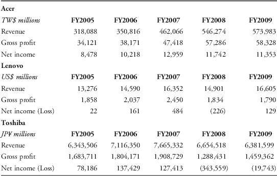
Solution to 1: Toshiba is far larger than the other two companies based on FY2009 revenues in US$. Toshiba’s FY2009 revenues of US$69.0 billion are far higher than either Acer’s US$17.8 billion or Lenovo’s US$16.6 billion.
Acer: At the assumed average exchange rate of 32.2 TW$/US$, Acer’s FY2009 revenues are equivalent to US$17.8 billion (=TW$573.983billion÷32.2 TW$/US$).
Lenovo: Lenovo’s FY2009 revenues totaled US$16.6 billion.
Toshiba: At the assumed average exchange rate of 92.5 JP¥/US$, Toshiba’s revenues for FY2009 are equivalent to US$69.0 billion (=JPY 6,381.599 billion÷92.5 JP¥/US$).
Note: Comparing the size of companies reporting in different currencies requires translating reported numbers into a common currency using exchange rates at some point in time. This solution converts the revenues of Acer and Toshiba to billions of U.S. dollars using the average exchange rate of the fiscal period. It would be equally informative (and would yield the same conclusion) to convert the revenues of Acer and Lenovo to Japanese yen, or to convert the revenues of Toshiba and Lenovo to New Taiwan dollars.
Solution to 2: The growth in Acer’s revenue was much higher than either of the other two companies.
| Change in Revenue FY2009 versus FY2005 | Compound Annual Growth Rate from FY2005 to FY2009 | |
| Acer | 80.4% | 15.9% |
| Lenovo | 25.1% | 5.8% |
| Toshiba | 0.6% | 0.1% |
The table shows two growth metrics. Calculations are illustrated using the revenue data for Acer:
The change in Acer’s revenue for FY2009 versus FY2005 is 80.4 percent calculated as (573,983−318,088)÷318,088 or equivalently (573,983÷318,088)–1.
The compound annual growth rate in Acer’s revenue from FY2005 to FY2009 is 15.9 percent, calculated using a financial calculator with the following inputs: Present Value=−318,088; Future value=573,983; N=4; Payment=0; and then Interest=? to solve for growth.
Calculation of the compound annual growth rate can also be expressed as follows: [(Ending value÷Beginning value)(1/number of periods)]−1=[(573,983÷318,088)(1/4) − 1=0.159 or 15.9 percent.
Solution to 3: Profitability can be assessed by comparing the amount of gross profit to revenue and the amount of net income to revenue. The following table presents these two profitability ratios—gross profit margin (gross profit divided by revenue) and net profit margin (net income divided by revenue)—for each year.
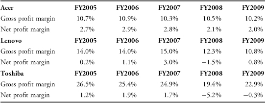
The net profit margins indicate that Acer has been the most profitable of the three companies. The company’s net profit margin was somewhat lower in the most recent two years (only 2.1 percent and 2.0 percent in FY2008 and FY2009, respectively, compared to 2.7 percent, 2.9 percent, and 2.8 percent in FYs 2005, 2006, and 2007, respectively), but has nonetheless remained positive and has remained higher than the competing companies.
Acer’s gross profit margin has remained consistently above 10 percent in all five fiscal years. In contrast, Lenovo’s gross profit margin has declined markedly over the five-year period, but remains higher than Acer’s, which is consistent with the company’s strategic objective to achieve higher selling prices by stressing the high engineering quality of its personal computers. However, Lenovo’s net profit margin has typically been lower than Acer’s. Further analysis is needed to determine the cause of Lenovo’s gross profitability decline over the period FY2005 to 2009 (lower selling prices and/or higher costs), to assess whether this decline is likely to persist in future years, and to determine the reason Lenovo’s net profit margins are generally lower than Acer’s despite Lenovo’s higher gross profit margins.
Because Toshiba is a conglomerate, profit ratios based on data for the entire company give limited information about the company’s personal computer business. Ratios based on segment data would likely be more useful than profit ratios for the entire company. Based on the aggregate information, Toshiba’s gross profit margins are higher than either Acer’s or Lenovo’s gross profit margins, whereas Toshiba’s net profit margins are generally lower than the net profit margins of either of the other two companies.
Section 3.1 describes the tools and techniques of ratio analysis in more detail. Sections 3.2 to 3.4 describe other tools and techniques.
3.1. Ratios
There are many relationships between financial accounts and between expected relationships from one point in time to another. Ratios are a useful way of expressing these relationships. Ratios express one quantity in relation to another (usually as a quotient).
Extensive academic research has examined the importance of ratios in predicting stock returns (Ou and Penman, 1989; Abarbanell and Bushee, 1998) or credit failure (Altman, 1968; Ohlson, 1980; Hopwood et al., 1994). This research has found that financial statement ratios are effective in selecting investments and in predicting financial distress. Practitioners routinely use ratios to derive and communicate the value of companies and securities.
Several aspects of ratio analysis are important to understand. First, the computed ratio is not “the answer.” The ratio is an indicator of some aspect of a company’s performance, telling what happened but not why it happened. For example, an analyst might want to answer the question: Which of two companies was more profitable? As demonstrated in the previous example, the net profit margin, which expresses profit relative to revenue, can provide insight into this question. Net profit margin is calculated by dividing net income by revenue:4
![]()
Assume Company A has €100,000 of net income and Company B has €200,000 of net income. Company B generated twice as much income as Company A, but was it more profitable? Assume further that Company A has €2,000,000 of revenue, and thus a net profit margin of 5 percent, and Company B has €6,000,000 of revenue, and thus a net profit margin of 3.33 percent. Expressing net income as a percentage of revenue clarifies the relationship: For each €100 of revenue, Company A earns €5 in net income, whereas Company B earns only €3.33 for each €100 of revenue. So, we can now answer the question of which company was more profitable in percentage terms: Company A was more profitable, as indicated by its higher net profit margin of 5 percent. Note that Company A was more profitable despite the fact that Company B reported higher absolute amounts of net income and revenue. However, this ratio by itself does not tell us why Company A has a higher profit margin. Further analysis is required to determine the reason (perhaps higher relative sales prices or better cost control or lower effective tax rates).
Company size sometimes confers economies of scale, so the absolute amounts of net income and revenue are useful in financial analysis. However, ratios reduce the effect of size, which enhances comparisons between companies and over time.
A second important aspect of ratio analysis is that differences in accounting policies (across companies and across time) can distort ratios, and a meaningful comparison may, therefore, involve adjustments to the financial data. Third, not all ratios are necessarily relevant to a particular analysis. The ability to select a relevant ratio or ratios to answer the research question is an analytical skill. Finally, as with financial analysis in general, ratio analysis does not stop with computation; interpretation of the result is essential. In practice, differences in ratios across time and across companies can be subtle, and interpretation is situation specific.
3.1.1. The Universe of Ratios
There are no authoritative bodies specifying exact formulas for computing ratios or providing a standard, comprehensive list of ratios. Formulas and even names of ratios often differ from analyst to analyst or from database to database. The number of different ratios that can be created is practically limitless. There are, however, widely accepted ratios that have been found to be useful. Section 4 of this chapter will focus primarily on these broad classes and commonly accepted definitions of key ratios. However, the analyst should be aware that different ratios may be used in practice and that certain industries have unique ratios tailored to the characteristics of that industry. When faced with an unfamiliar ratio, the analyst can examine the underlying formula to gain insight into what the ratio is measuring. For example, consider the following ratio formula:
![]()
Never having seen this ratio, an analyst might question whether a result of 12 percent is better than 8 percent. The answer can be found in the ratio itself. The numerator is operating income and the denominator is average total assets, so the ratio can be interpreted as the amount of operating income generated per unit of assets. For every €100 of average total assets, generating €12 of operating income is better than generating €8 of operating income. Furthermore, it is apparent that this particular ratio is an indicator of profitability (and, to a lesser extent, efficiency in use of assets in generating operating profits). When facing a ratio for the first time, the analyst should evaluate the numerator and denominator to assess what the ratio is attempting to measure and how it should be interpreted. This is demonstrated in Example 7-3.
EXAMPLE 7-3 Interpreting a Financial Ratio
A U.S. insurance company reports that its “combined ratio” is determined by dividing losses and expenses incurred by net premiums earned. It reports the following combined ratios:

Explain what this ratio is measuring and compare the results reported for each of the years shown in the chart. What other information might an analyst want to review before making any conclusions on this information?
Solution: The combined ratio is a profitability measure. The ratio is explaining how much costs (losses and expenses) were incurred for every dollar of revenue (net premiums earned). The underlying formula indicates that a lower ratio is better. The Year 5 ratio of 90.1 percent means that for every dollar of net premiums earned, the costs were $0.901, yielding a gross profit of $0.099. Ratios greater than 100 percent indicate an overall loss. A review of the data indicates that there does not seem to be a consistent trend in this ratio. Profits were achieved in Years 5 and 3. The results for Years 4 and 2 show the most significant costs at approximately 104 percent.
The analyst would want to discuss this data further with management and understand the characteristics of the underlying business. He or she would want to understand why the results are so volatile. The analyst would also want to determine what should be used as a benchmark for this ratio.
The Operating income/Average total assets ratio shown previously is one of many versions of the return on assets (ROA) ratio. Note that there are other ways of specifying this formula based on how assets are defined. Some financial ratio databases compute ROA using the ending value of assets rather than average assets. In limited cases, one may also see beginning assets in the denominator. Which one is right? It depends on what you are trying to measure and the underlying company trends. If the company has a stable level of assets, the answer will not differ greatly under the three measures of assets (beginning, average, and ending). However, if the assets are growing (or shrinking), the results will differ among the three measures. When assets are growing, operating income divided by ending assets may not make sense because some of the income would have been generated before some assets were purchased, and this would understate the company’s performance. Similarly, if beginning assets are used, some of the operating income later in the year may have been generated only because of the addition of assets; therefore, the ratio would overstate the company’s performance. Because operating income occurs throughout the period, it generally makes sense to use some average measure of assets. A good general rule is that when an income statement or cash flow statement number is in the numerator of a ratio and a balance sheet number is in the denominator, then an average should be used for the denominator. It is generally not necessary to use averages when only balance sheet numbers are used in both the numerator and denominator because both are determined as of the same date. However, in some instances, even ratios that only use balance sheet data may use averages. For example, return on equity (ROE), which is defined as net income divided by average shareholders’ equity, can be decomposed into other ratios, some of which only use balance sheet data. In decomposing ROE into component ratios, if an average is used in one of the component ratios then it should be used in the other component ratios. The decomposition of ROE is discussed further in Section 4.6.2.
If an average is used, judgment is also required about what average should be used. For simplicity, most ratio databases use a simple average of the beginning and end-of-year balance sheet amounts. If the company’s business is seasonal so that levels of assets vary by interim period (semiannual or quarterly), then it may be beneficial to take an average over all interim periods, if available. (If the analyst is working within a company and has access to monthly data, this can also be used.)
3.1.2. Value, Purposes, and Limitations of Ratio Analysis
The value of ratio analysis is that it enables a financial analyst to evaluate past performance, assess the current financial position of the company, and gain insights useful for projecting future results. As noted previously, the ratio itself is not “the answer” but is an indicator of some aspect of a company’s performance. Financial ratios provide insights into:
- Microeconomic relationships within a company that help analysts project earnings and free cash flow.
- A company’s financial flexibility, or ability to obtain the cash required to grow and meet its obligations, even if unexpected circumstances develop.
- Management’s ability.
- Changes in the company and/or industry over time.
- Comparability with peer companies or the relevant industry(ies).
There are also limitations to ratio analysis. Factors to consider include:
- The heterogeneity or homogeneity of a company’s operating activities. Companies may have divisions operating in many different industries. This can make it difficult to find comparable industry ratios to use for comparison purposes.
- The need to determine whether the results of the ratio analysis are consistent. One set of ratios may indicate a problem, whereas another set may indicate that the potential problem is only short term in nature.
- The need to use judgment. A key issue is whether a ratio for a company is within a reasonable range. Although financial ratios are used to help assess the growth potential and risk of a company, they cannot be used alone to directly value a company or its securities, or to determine its creditworthiness. The entire operation of the company must be examined, and the external economic and industry setting in which it is operating must be considered when interpreting financial ratios.
- The use of alternative accounting methods. Companies frequently have latitude when choosing certain accounting methods. Ratios taken from financial statements that employ different accounting choices may not be comparable unless adjustments are made. Some important accounting considerations include the following:
- FIFO (first in, first out), LIFO (last in, first out), or average cost inventory valuation methods (IFRS does not allow LIFO).
- Cost or equity methods of accounting for unconsolidated affiliates.
- Straight line or accelerated methods of depreciation.
- Capital or operating lease treatment.
The expanding use of IFRS and the ongoing convergence between IFRS and U.S. GAAP seeks to make the financial statements of different companies comparable and may overcome some of these difficulties. Nonetheless, there will remain accounting choices that the analyst must consider.
3.1.3. Sources of Ratios
Ratios may be computed using data obtained directly from companies’ financial statements or from a database such as Bloomberg, Compustat, FactSet, or Thomson Reuters. The information provided by the database may include information as reported in companies’ financial statements and ratios calculated based on the information. These databases are popular because they provide easy access to many years of historical data so that trends over time can be examined. They also allow for ratio calculations based on periods other than the company’s fiscal year, such as for the trailing 12 months (TTM) or most recent quarter (MRQ).
EXAMPLE 7-4 Trailing Twelve Months
On 15 July, an analyst is examining a company with a fiscal year ending on 31 December. Use the following data to calculate the company’s trailing 12-month earnings (for the period ended 30 June 2010).
- Earnings for the year ended 31 December, 2009: $1,200
- Earnings for the six months ended 30 June 2009: $550
- Earnings for the six months ended 30 June 2010: $750
Solution: The company’s trailing 12 months earnings is $1,400, calculated as $1,200 − $550=$750.
Analysts should be aware that the underlying formulas for ratios may differ by vendor. The formula used should be obtained from the vendor, and the analyst should determine whether any adjustments are necessary. Furthermore, database providers often exercise judgment when classifying items. For example, operating income may not appear directly on a company’s income statement, and the vendor may use judgment to classify income statement items as “operating” or “nonoperating.” Variation in such judgments would affect any computation involving operating income. It is therefore a good practice to use the same source for data when comparing different companies or when evaluating the historical record of a single company. Analysts should verify the consistency of formulas and data classifications by the data source. Analysts should also be mindful of the judgments made by a vendor in data classifications and refer back to the source financial statements until they are comfortable that the classifications are appropriate.
Systems are under development that collect financial data from regulatory filings and can automatically compute ratios. The eXtensible Business Reporting Language (XBRL) is a mechanism that attaches “smart tags” to financial information (e.g., total assets), so that software can automatically collect the data and perform desired computations. The organization developing XBRL (www.xbrl.org) is an international nonprofit consortium of over 600 members from companies, associations, and agencies, including the International Accounting Standards Board. Many stock exchanges and regulatory agencies around the world now use XBRL for receiving and distributing public financial reports from listed companies.
Analysts can compare a subject company to similar (peer) companies in these databases or use aggregate industry data. For nonpublic companies, aggregate industry data can be obtained from such sources as Annual Statement Studies by the Risk Management Association or Dun & Bradstreet. These publications typically provide industry data with companies sorted into quartiles. By definition, 25 percent of companies’ ratios fall within the lowest quartile, 25 percent have ratios between the lower quartile and median value, and so on. Analysts can then determine a company’s relative standing in the industry.
3.2. Common-Size Analysis
Common-size analysis involves expressing financial data, including entire financial statements, in relation to a single financial statement item, or base. Items used most frequently as the bases are total assets or revenue. In essence, common-size analysis creates a ratio between every financial statement item and the base item.
Common-size analysis was demonstrated in chapters for the income statement, balance sheet, and cash flow statement. In this section, we present common-size analysis of financial statements in greater detail and include further discussion of their interpretation.
3.2.1. Common-Size Analysis of the Balance Sheet
A vertical5 common-size balance sheet, prepared by dividing each item on the balance sheet by the same period’s total assets and expressing the results as percentages, highlights the composition of the balance sheet. What is the mix of assets being used? How is the company financing itself? How does one company’s balance sheet composition compare with that of peer companies, and what are the reasons for any differences?
A horizontal common-size balance sheet, prepared by computing the increase or decrease in percentage terms of each balance sheet item from the prior year or prepared by dividing the quantity of each item by a base year quantity of the item, highlights changes in items. These changes can be compared to expectations. The following section on trend analysis will illustrate a horizontal common-size balance sheet.
Exhibit 7-3 presents a vertical common-size (partial) balance sheet for a hypothetical company in two time periods. In this example, receivables have increased from 35 percent to 57 percent of total assets and the ratio has increased by 63 percent from Period 1 to Period 2. What are possible reasons for such an increase? The increase might indicate that the company is making more of its sales on a credit basis rather than a cash basis, perhaps in response to some action taken by a competitor. Alternatively, the increase in receivables as a percentage of assets may have occurred because of a change in another current asset category, for example, a decrease in the level of inventory; the analyst would then need to investigate why that asset category has changed. Another possible reason for the increase in receivables as a percentage of assets is that the company has lowered its credit standards, relaxed its collection procedures, or adopted more aggressive revenue recognition policies. The analyst can turn to other comparisons and ratios (e.g., comparing the rate of growth in accounts receivable with the rate of growth in sales) to help determine which explanation is most likely.
EXHIBIT 7-3 Vertical Common-Size (Partial) Balance Sheet for a Hypothetical Company
| Period 1 Percent of Total Assets | Period 2 Percent of Total Assets | |
| Cash | 25 | 15 |
| Receivables | 35 | 57 |
| Inventory | 35 | 20 |
| Fixed assets, net of depreciation | 5 | 8 |
| Total assets | 100 | 100 |
3.2.2. Common-Size Analysis of the Income Statement
A vertical common-size income statement divides each income statement item by revenue, or sometimes by total assets (especially in the case of financial institutions). If there are multiple revenue sources, a decomposition of revenue in percentage terms is useful. Exhibit 7-4 presents a hypothetical company’s vertical common-size income statement in two time periods. Revenue is separated into the company’s four services, each shown as a percentage of total revenue.
In this example, revenues from Service A have become a far greater percentage of the company’s total revenue (30 percent in Period 1 and 45 percent in Period 2). What are possible reasons for and implications of this change in business mix? Did the company make a strategic decision to sell more of Service A, perhaps because it is more profitable? Apparently not, because the company’s earnings before interest, taxes, depreciation, and amortization (EBITDA) declined from 53 percent of sales to 45 percent, so other possible explanations should be examined. In addition, we note from the composition of operating expenses that the main reason for this decline in profitability is that salaries and employee benefits have increased from 15 percent to 25 percent of total revenue. Are more highly compensated employees required for Service A? Were higher training costs incurred in order to increase revenues from Service A? If the analyst wants to predict future performance, the causes of these changes must be understood.
In addition, Exhibit 7-4 shows that the company’s income tax as a percentage of sales has declined dramatically (from 15 percent to 8 percent). Furthermore, taxes as a percentage of earnings before tax (EBT) (the effective tax rate, which is usually the more relevant comparison), have decreased from 36 percent (= 15/42) to 24 percent (= 8/34). Is Service A, which in Period 2 is a greater percentage of total revenue, provided in a jurisdiction with lower tax rates? If not, what is the explanation for the change in effective tax rate?
The observations based on Exhibit 7-4 summarize the issues that can be raised through analysis of the vertical common-size income statement.
EXHIBIT 7-4 Vertical Common-Size Income Statement for Hypothetical Company
| Period 1 Percent of Total Revenue | Period 2 Percent of Total Revenue | |
| Revenue source: Service A | 30 | 45 |
| Revenue source: Service B | 23 | 20 |
| Revenue source: Service C | 30 | 30 |
| Revenue source: Service D | 17 | 5 |
| Total revenue | 100 | 100 |
| Operating expenses (excluding depreciation) | ||
| Salaries and employee benefits | 15 | 25 |
| Administrative expenses | 22 | 20 |
| Rent expense | 10 | 10 |
| EBITDA | 53 | 45 |
| Depreciation and amortization | 4 | 4 |
| EBIT | 49 | 41 |
| Interest paid | 7 | 7 |
| EBT | 42 | 34 |
| Income tax provision | 15 | 8 |
| Net income | 27 | 26 |
EBIT=earnings before interest and tax.
3.2.3. Cross-Sectional Analysis
As noted previously, ratios and common-size statements derive part of their meaning through comparison to some benchmark. Cross-sectional analysis (sometimes called “relative analysis”) compares a specific metric for one company with the same metric for another company or group of companies, allowing comparisons even though the companies might be of significantly different sizes and/or operate in different currencies. This is illustrated in Exhibit 7-5.
EXHIBIT 7-5 Vertical Common-Size (Partial) Balance Sheet for Two Hypothetical Companies
| Assets | Company 1 Percent of Total Assets | Company 2 Percent of Total Assets |
| Cash | 38 | 12 |
| Receivables | 33 | 55 |
| Inventory | 27 | 24 |
| Fixed assets net of depreciation | 1 | 2 |
| Investments | 1 | 7 |
| Total Assets | 100 | 100 |
Exhibit 7-5 presents a vertical common-size (partial) balance sheet for two hypothetical companies at the same point in time. Company 1 is clearly more liquid (liquidity is a function of how quickly assets can be converted into cash) than Company 2, which has only 12 percent of assets available as cash, compared with the highly liquid Company 1, which has 38 percent of assets available as cash. Given that cash is generally a relatively low-yielding asset and thus not a particularly efficient use of excess funds, why does Company 1 hold such a large percentage of total assets in cash? Perhaps the company is preparing for an acquisition, or maintains a large cash position as insulation from a particularly volatile operating environment. Another issue highlighted by the comparison in this example is the relatively high percentage of receivables in Company 2’s assets, which may indicate a greater proportion of credit sales, overall changes in asset composition, lower credit or collection standards, or aggressive accounting policies.
3.2.4. Trend Analysis6
When looking at financial statements and ratios, trends in the data, whether they are improving or deteriorating, are as important as the current absolute or relative levels. Trend analysis provides important information regarding historical performance and growth and, given a sufficiently long history of accurate seasonal information, can be of great assistance as a planning and forecasting tool for management and analysts.
Exhibit 7-6A presents a partial balance sheet for a hypothetical company over five periods. The last two columns of the table show the changes for Period 5 compared with Period 4, expressed both in absolute currency (in this case, dollars) and in percentages. A small percentage change could hide a significant currency change and vice versa, prompting the analyst to investigate the reasons despite one of the changes being relatively small. In this example, the largest percentage change was in investments, which decreased by 33.3 percent.7 However, an examination of the absolute currency amount of changes shows that investments changed by only $2 million, and the more significant change was the $12 million increase in receivables.
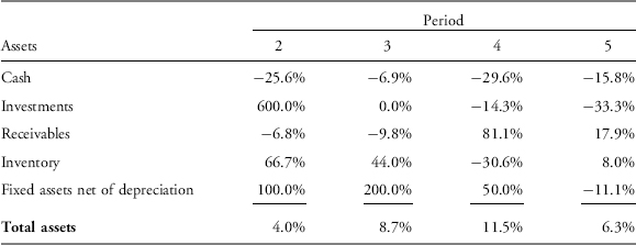
Another way to present data covering a period of time is to show each item in relation to the same item in a base year (i.e., a horizontal common-size balance sheet). Exhibits 7-6B and 7-6C illustrate alternative presentations of horizontal common-size balance sheets. Exhibit 7-6B presents the information from the same partial balance sheet as in Exhibit 7-6A, but indexes each item relative to the same item in Period 1. For example, in Period 2, the company had $29 million cash, which is 74 percent or 0.74 of the amount of cash it had in Period 1. Expressed as an index relative to Period 1, where each item in Period 1 is given a value of 1.00, the value in Period 2 would be 0.74 ($29/$39=0.74). In Period 3, the company had $27 million cash, which is 69 percent of the amount of cash it had in Period 1 ($27/$39=0.69).
Exhibit 7-6C presents the percentage change in each item, relative to the previous year. For example, the change in cash from Period 1 to Period 2 was −25.6 percent ($29/$39 − 1=–0.256), and the change in cash from Period 2 to Period 3 was −6.9 percent ($27/$29 − 1=–0.069). An analyst will select the horizontal common-size balance that addresses the particular period of interest. Exhibit 7-6B clearly highlights that in Period 5 compared to Period 1, the company has less than half the amount of cash, four times the amount of investments, and eight times the amount of property, plant, and equipment. Exhibit 7-6C highlights year-to-year changes: For example, cash has declined in each period. Presenting data this way highlights significant changes. Again, note that a mathematically big change is not necessarily an important change. For example, fixed assets increased 100 percent, i.e., doubled between Period 1 and 2; however, as a proportion of total assets, fixed assets increased from 1 percent of total assets to 2 percent of total assets. The company’s working capital assets (receivables and inventory) are a far higher proportion of total assets and would likely warrant more attention from an analyst.
An analysis of horizontal common-size balance sheets highlights structural changes that have occurred in a business. Past trends are obviously not necessarily an accurate predictor of the future, especially when the economic or competitive environment changes. An examination of past trends is more valuable when the macroeconomic and competitive environments are relatively stable and when the analyst is reviewing a stable or mature business. However, even in less stable contexts, historical analysis can serve as a basis for developing expectations. Understanding of past trends is helpful in assessing whether these trends are likely to continue or if the trend is likely to change direction.
EXHIBIT 7-6A Partial Balance Sheet for a Hypothetical Company over Five Periods
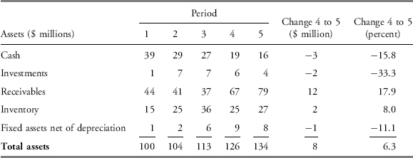
EXHIBIT 7-6B Horizontal Common-Size (Partial) Balance Sheet for a Hypothetical Company over Five Periods, with Each Item Expressed Relative to the Same Item in Period One
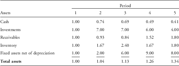
EXHIBIT 7-6C Horizontal Common-Size (Partial) Balance Sheet for a Hypothetical Company over Five Periods, with Percent Change in Each Item Relative to the Prior Period
One measure of success is for a company to grow at a rate greater than the rate of the overall market in which it operates. Companies that grow slowly may find themselves unable to attract equity capital. Conversely, companies that grow too quickly may find that their administrative and management information systems cannot keep up with the rate of expansion.
3.2.5. Relationships among Financial Statements
Trend data generated by a horizontal common-size analysis can be compared across financial statements. For example, the growth rate of assets for the hypothetical company in Exhibit 7-6 can be compared with the company’s growth in revenue over the same period of time. If revenue is growing more quickly than assets, the company may be increasing its efficiency (i.e., generating more revenue for every dollar invested in assets).
As another example, consider the following year-over-year percentage changes for a hypothetical company:
| Revenue | +20% |
| Net income | +25% |
| Operating cash flow | −10% |
| Total assets | +30% |
Net income is growing faster than revenue, which indicates increasing profitability. However, the analyst would need to determine whether the faster growth in net income resulted from continuing operations or from nonoperating, nonrecurring items. In addition, the 10 percent decline in operating cash flow despite increasing revenue and net income clearly warrants further investigation because it could indicate a problem with earnings quality (perhaps aggressive reporting of revenue). Lastly, the fact that assets have grown faster than revenue indicates the company’s efficiency may be declining. The analyst should examine the composition of the increase in assets and the reasons for the changes. Example 7-5 illustrates a company where comparisons of trend data from different financial statements were actually indicative of aggressive accounting policies.
EXAMPLE 7-5 Use of Comparative Growth Information8
In July 1996, Sunbeam, a U.S. company, brought in new management to turn the company around. In the following year, 1997, using 1996 as the base, the following was observed based on reported numbers:
| Revenue | +19% |
| Inventory | +58% |
| Receivables | +38% |
It is generally more desirable to observe inventory and receivables growing at a slower (or similar) rate compared to revenue growth. Receivables growing faster than revenue can indicate operational issues, such as lower credit standards or aggressive accounting policies for revenue recognition. Similarly, inventory growing faster than revenue can indicate an operational problem with obsolescence or aggressive accounting policies, such as an improper overstatement of inventory to increase profits.
In this case, the explanation lay in aggressive accounting policies. Sunbeam was later charged by the U.S. Securities and Exchange Commission with improperly accelerating the recognition of revenue and engaging in other practices, such as billing customers for inventory prior to shipment.
3.3. The Use of Graphs as an Analytical Tool
Graphs facilitate comparison of performance and financial structure over time, highlighting changes in significant aspects of business operations. In addition, graphs provide the analyst (and management) with a visual overview of risk trends in a business. Graphs may also be used effectively to communicate the analyst’s conclusions regarding financial condition and risk management aspects.
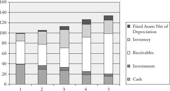
Exhibit 7-7 presents the information from Exhibit 7-6A in a stacked column format. The graph makes the significant decline in cash and growth in receivables (both in absolute terms and as a percentage of assets) readily apparent. In Exhibit 7-7, the vertical axis shows US$ millions and the horizontal axis denotes the period.
Choosing the appropriate graph to communicate the most significant conclusions of a financial analysis is a skill. In general, pie graphs are most useful to communicate the composition of a total value (e.g., assets over a limited amount of time, say one or two periods). Line graphs are useful when the focus is on the change in amount for a limited number of items over a relatively longer time period. When the composition and amounts, as well as their change over time, are all important, a stacked column graph can be useful.
EXHIBIT 7-7 Stacked Column Graph of Asset Composition of Hypothetical Company over Five Periods
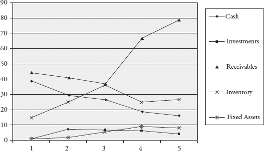
When comparing Period 5 with Period 4, the growth in receivables appears to be within normal bounds; but when comparing Period 5 with earlier periods, the dramatic growth becomes apparent. In the same manner, a simple line graph will also illustrate the growth trends in key financial variables. Exhibit 7-8 presents the information from Exhibit 7-6A as a line graph, illustrating the growth of assets of a hypothetical company over five periods. The steady decline in cash, volatile movements of inventory, and dramatic growth of receivables is clearly illustrated. Again, the vertical axis is shown in US$ millions and the horizontal axis denotes periods.
EXHIBIT 7-8 Line Graph of Growth of Assets of Hypothetical Company over Five Periods
3.4. Regression Analysis
When analyzing the trend in a specific line item or ratio, frequently it is possible simply to visually evaluate the changes. For more complex situations, regression analysis can help identify relationships (or correlation) between variables. For example, a regression analysis could relate a company’s sales to GDP over time, providing insight into whether the company is cyclical. In addition, the statistical relationship between sales and GDP could be used as a basis for forecasting sales.
Other examples include the relationship between a company’s sales and inventory over time, or the relationship between hotel occupancy and a company’s hotel revenues. In addition to providing a basis for forecasting, regression analysis facilitates identification of items or ratios that are not behaving as expected, given historical statistical relationships.
4. COMMON RATIOS USED IN FINANCIAL ANALYSIS
In the previous section, we focused on ratios resulting from common-size analysis. In this section, we expand the discussion to include other commonly used financial ratios and the broad classes into which they are categorized. There is some overlap with common-size financial statement ratios. For example, a common indicator of profitability is the net profit margin, which is calculated as net income divided by sales. This ratio appears on a vertical common-size income statement. Other ratios involve information from multiple financial statements or even data from outside the financial statements.
Because of the large number of ratios, it is helpful to think about ratios in terms of broad categories based on what aspects of performance a ratio is intended to detect. Financial analysts and data vendors use a variety of categories to classify ratios. The category names and the ratios included in each category can differ. Common ratio categories include activity, liquidity, solvency, profitability, and valuation. These categories are summarized in Exhibit 7-9. Each category measures a different aspect of the company’s business, but all are useful in evaluating a company’s overall ability to generate cash flows from operating its business and the associated risks.
EXHIBIT 7-9 Categories of Financial Ratios
| Category | Description |
| Activity | Activity ratios measure how efficiently a company performs day-to-day tasks, such as the collection of receivables and management of inventory. |
| Liquidity | Liquidity ratios measure the company’s ability to meet its short-term obligations. |
| Solvency | Solvency ratios measure a company’s ability to meet long-term obligations. Subsets of these ratios are also known as “leverage” and “long-term debt” ratios. |
| Profitability | Profitability ratios measure the company’s ability to generate profits from its resources (assets). |
| Valuation | Valuation ratios measure the quantity of an asset or flow (e.g., earnings) associated with ownership of a specified claim (e.g., a share or ownership of the enterprise). |
These categories are not mutually exclusive; some ratios are useful in measuring multiple aspects of the business. For example, an activity ratio measuring how quickly a company collects accounts receivable is also useful in assessing the company’s liquidity because collection of revenues increases cash. Some profitability ratios also reflect the operating efficiency of the business. In summary, analysts appropriately use certain ratios to evaluate multiple aspects of the business. Analysts also need to be aware of variations in industry practice in the calculation of financial ratios. In the text that follows, alternative views on ratio calculations are often provided.
4.1. Interpretation and Context
Financial ratios can only be interpreted in the context of other information, including benchmarks. In general, the financial ratios of a company are compared with those of its major competitors (cross-sectional and trend analysis) and to the company’s prior periods (trend analysis). The goal is to understand the underlying causes of divergence between a company’s ratios and those of the industry. Even ratios that remain consistent require understanding because consistency can sometimes indicate accounting policies selected to smooth earnings. An analyst should evaluate financial ratios based on the following:
1. Company goals and strategy: Actual ratios can be compared with company objectives to determine whether objectives are being attained and whether the results are consistent with the company’s strategy.
2. Industry norms (cross-sectional analysis): A company can be compared with others in its industry by relating its financial ratios to industry norms or to a subset of the companies in an industry. When industry norms are used to make judgments, care must be taken because:
- Many ratios are industry specific, and not all ratios are important to all industries.
- Companies may have several different lines of business. This will cause aggregate financial ratios to be distorted. It is better to examine industry-specific ratios by lines of business.
- Differences in accounting methods used by companies can distort financial ratios.
- Differences in corporate strategies can affect certain financial ratios.
3. Economic conditions: For cyclical companies, financial ratios tend to improve when the economy is strong and weaken during recessions. Therefore, financial ratios should be examined in light of the current phase of the business cycle.
The following sections discuss activity, liquidity, solvency, and profitability ratios in turn. Selected valuation ratios are presented later in the section on equity analysis.
4.2. Activity Ratios
Activity ratios are also known as asset utilization ratios or operating efficiency ratios. This category is intended to measure how well a company manages various activities, particularly how efficiently it manages its various assets. Activity ratios are analyzed as indicators of ongoing operational performance—how effectively assets are used by a company. These ratios reflect the efficient management of both working capital and longer-term assets. As noted, efficiency has a direct impact on liquidity (the ability of a company to meet its short-term obligations), so some activity ratios are also useful in assessing liquidity.
4.2.1. Calculation of Activity Ratios
Exhibit 7-10 presents the most commonly used activity ratios. The exhibit shows the numerator and denominator of each ratio.
EXHIBIT 7-10 Definitions of Commonly Used Activity Ratios
| Activity Ratios | Numerator | Denominator |
| Inventory turnover | Cost of sales or cost of goods sold | Average inventory |
| Days of inventory on hand (DOH) | Number of days in period | Inventory turnover |
| Receivables turnover | Revenue | Average receivables |
| Days of sales outstanding (DSO) | Number of days in period | Receivables turnover |
| Payables turnover | Purchases | Average trade payables |
| Number of days of payables | Number of days in period | Payables turnover |
| Working capital turnover | Revenue | Average working capital |
| Fixed asset turnover | Revenue | Average net fixed assets |
| Total asset turnover | Revenue | Average total assets |
Activity ratios measure how efficiently the company utilizes assets. They generally combine information from the income statement in the numerator with balance sheet items in the denominator. Because the income statement measures what happened during a period whereas the balance sheet shows the condition only at the end of the period, average balance sheet data are normally used for consistency. For example, to measure inventory management efficiency, cost of sales or cost of goods sold (from the income statement) is divided by average inventory (from the balance sheet). Most databases, such as Bloomberg and Baseline, use this averaging convention when income statement and balance sheet data are combined. These databases typically average only two points: the beginning of the year and the end of the year. The examples that follow based on annual financial statements illustrate that practice. However, some analysts prefer to average more observations if they are available, especially if the business is seasonal. If a semiannual report is prepared, an average can be taken over three data points (beginning, middle, and end of year). If quarterly data are available, a five-point average can be computed (beginning of year and end of each quarterly period) or a four-point average using the end of each quarterly period. Note that if the company’s year ends at a low or high point for inventory for the year, there can still be bias in using three or five data points, because the beginning and end of year occur at the same time of the year and are effectively double counted.
Because cost of goods sold measures the cost of inventory that has been sold, this ratio measures how many times per year the entire inventory was theoretically turned over, or sold. (We say that the entire inventory was “theoretically” sold because in practice companies do not generally sell out their entire inventory.) If, for example, a company’s cost of goods sold for a recent year was €120,000 and its average inventory was €10,000, the inventory turnover ratio would be 12. The company theoretically turns over (i.e., sells) its entire inventory 12 times per year (i.e., once a month). (Again, we say “theoretically” because in practice the company likely carries some inventory from one month into another.) Turnover can then be converted to days of inventory on hand (DOH) by dividing inventory turnover into the number of days in the accounting period. In this example, the result is a DOH of 30.42 (365/12), meaning that, on average, the company’s inventory was on hand for about 30 days, or, equivalently, the company kept on hand about 30 days’ worth of inventory, on average, during the period.
Activity ratios can be computed for any annual or interim period, but care must be taken in the interpretation and comparison across periods. For example, if the same company had cost of goods sold for the first quarter (90 days) of the following year of €35,000 and average inventory of €11,000, the inventory turnover would be 3.18 times. However, this turnover rate is 3.18 times per quarter, which is not directly comparable to the 12 times per year in the preceding year. In this case, we can annualize the quarterly inventory turnover rate by multiplying the quarterly turnover by 4 (12 months/3 months; or by 4.06, using 365 days/90 days) for comparison to the annual turnover rate. So, the quarterly inventory turnover is equivalent to a 12.72 annual inventory turnover (or 12.91 if we annualize the ratio using a 90-day quarter and a 365-day year). To compute the DOH using quarterly data, we can use the quarterly turnover rate and the number of days in the quarter for the numerator—or, we can use the annualized turnover rate and 365 days; either results in DOH of around 28.3, with slight differences due to rounding (90/3.18=28.30 and 365/12.91=28.27). Another time-related computational detail is that for companies using a 52/53-week annual period and for leap years, the actual days in the year should be used rather than 365.
In some cases, an analyst may want to know how many days of inventory are on hand at the end of the year rather than the average for the year. In this case, it would be appropriate to use the year-end inventory balance in the computation rather than the average. If the company is growing rapidly or if costs are increasing rapidly, analysts should consider using cost of goods sold just for the fourth quarter in this computation because the cost of goods sold of earlier quarters may not be relevant. Example 7-6 further demonstrates computation of activity ratios using Hong Kong Exchange–listed Lenovo Group Limited.
EXAMPLE 7-6 Computation of Activity Ratios
An analyst would like to evaluate Lenovo Group’s efficiency in collecting its trade accounts receivable during the fiscal year ended 31 March 2010 (FY2009). The analyst gathers the following information from Lenovo’s annual and interim reports:
| US$ in Thousands | |
| Trade receivables as of 31 March 2009 | 482,086 |
| Trade receivables as of 31 March 2010 | 1,021,062 |
| Revenue for year ended 31 March 2010 | 16,604,815 |
Calculate Lenovo’s receivables turnover and number of days of sales outstanding (DSO) for the fiscal year ended 31 March 2010.
Solution.
| Receivables turnover | = Revenue/Average receivables = 16,604,815/ [(1,021,062 + 482,086)/2] = 16,604,815/751,574 = 22.0934 times, or 22.1 rounded |
| DSO | = Number of days in period/Receivables turnover = 365/22.1 = 16.5 days |
On average, it took Lenovo 16.5 days to collect receivables during the fiscal year ended 31 March 2010.
4.2.2. Interpretation of Activity Ratios
In the following section, we further discuss the activity ratios that were defined in Exhibit 7-10.
Inventory turnover and DOH. Inventory turnover lies at the heart of operations for many entities. It indicates the resources tied up in inventory (i.e., the carrying costs) and can, therefore, be used to indicate inventory management effectiveness. A higher inventory turnover ratio implies a shorter period that inventory is held, and thus a lower DOH. In general, inventory turnover and DOH should be benchmarked against industry norms.
A high inventory turnover ratio relative to industry norms might indicate highly effective inventory management. Alternatively, a high inventory turnover ratio (and commensurately low DOH) could possibly indicate the company does not carry adequate inventory, so shortages could potentially hurt revenue. To assess which explanation is more likely, the analyst can compare the company’s revenue growth with that of the industry. Slower growth combined with higher inventory turnover could indicate inadequate inventory levels. Revenue growth at or above the industry’s growth supports the interpretation that the higher turnover reflects greater inventory management efficiency.
A low inventory turnover ratio (and commensurately high DOH) relative to the rest of the industry could be an indicator of slow-moving inventory, perhaps due to technological obsolescence or a change in fashion. Again, comparing the company’s sales growth with the industry can offer insight.
Receivables turnover and DSO. The number of DSO represents the elapsed time between a sale and cash collection, reflecting how fast the company collects cash from customers to whom it offers credit. Although limiting the numerator to sales made on credit in the receivables turnover would be more appropriate, credit sales information is not always available to analysts; therefore, revenue as reported in the income statement is generally used as an approximation.
A relatively high receivables turnover ratio (and commensurately low DSO) might indicate highly efficient credit and collection. Alternatively, a high receivables turnover ratio could indicate that the company’s credit or collection policies are too stringent, suggesting the possibility of sales being lost to competitors offering more lenient terms. A relatively low receivables turnover ratio would typically raise questions about the efficiency of the company’s credit and collections procedures. As with inventory management, comparison of the company’s sales growth relative to the industry can help the analyst assess whether sales are being lost due to stringent credit policies. In addition, comparing the company’s estimates of uncollectible accounts receivable and actual credit losses with past experience and with peer companies can help assess whether low turnover reflects credit management issues. Companies often provide details of receivables aging (how much receivables have been outstanding by age). This can be used along with DSO to understand trends in collection, as demonstrated in Example 7-7.
EXAMPLE 7-7 Evaluation of an Activity Ratio
An analyst has computed the average DSO for Lenovo for fiscal years ended 31 March 2010 and 2009:
| 2010 | 2009 | |
| Days of sales outstanding | 16.5 | 15.2 |
Revenue increased from US$14.901 billion for fiscal year ended 31 March 2009 (FY2008) to US$16.605 billion for fiscal year ended 31 March 2010 (FY2009). The analyst would like to better understand the change in the company’s DSO from FY2008 to FY2009 and whether the increase is indicative of any issues with the customers’ credit quality. The analyst collects accounts receivable aging information from Lenovo’s annual reports and computes the percentage of accounts receivable by days outstanding. This information is presented in Exhibit 7-11.
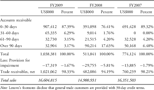
These data indicate that total accounts receivable more than doubled in FY2009 versus FY2008, while total sales increased by only 11.4 percent. This suggests that, overall, the company has been increasing customer financing to drive its sales growth. The significant increase in accounts receivable in total was the primary reason for the increase in DSO. The percentage of receivables older than 61 days has declined significantly which is generally positive. However, the large increase in 0–30 day receivables may be indicative of aggressive accounting policies or sales practices. Perhaps Lenovo offered incentives to generate a large amount of year-end sales. While the data may suggest that the quality of receivables improved in FY2009 versus FY2008, with a much lower percentage of receivables (and a much lower absolute amount) that are more than 90 days outstanding and, similarly, a lower percentage of estimated uncollectible receivables, this should be investigated further by the analyst.
Payables turn over and the number of days of payables. The number of days of payables reflects the average number of days the company takes to pay its suppliers, and the payables turnover ratio measures how many times per year the company theoretically pays off all its creditors. For purposes of calculating these ratios, an implicit assumption is that the company makes all its purchases using credit. If the amount of purchases is not directly available, it can be computed as cost of goods sold plus ending inventory less beginning inventory. Alternatively, cost of goods sold is sometimes used as an approximation of purchases.
A payables turnover ratio that is high (low days payable) relative to the industry could indicate that the company is not making full use of available credit facilities; alternatively, it could result from a company taking advantage of early payment discounts. An excessively low turnover ratio (high days payable) could indicate trouble making payments on time, or alternatively, exploitation of lenient supplier terms. This is another example where it is useful to look simultaneously at other ratios. If liquidity ratios indicate that the company has sufficient cash and other short-term assets to pay obligations and yet the days payable ratio is relatively high, the analyst would favor the lenient supplier credit and collection policies as an explanation.
Working capital turnover. Working capital is defined as current assets minus current liabilities. Working capital turnover indicates how efficiently the company generates revenue with its working capital. For example, a working capital turnover ratio of 4.0 indicates that the company generates €4 of revenue for every €1 of working capital. A high working capital turnover ratio indicates greater efficiency (i.e., the company is generating a high level of revenues relative to working capital). For some companies, working capital can be near zero or negative, rendering this ratio incapable of being interpreted. The following two ratios are more useful in those circumstances.
Fixed asset turnover. This ratio measures how efficiently the company generates revenues from its investments in fixed assets. Generally, a higher fixed asset turnover ratio indicates more efficient use of fixed assets in generating revenue. A low ratio can indicate inefficiency, a capital-intensive business environment, or a new business not yet operating at full capacity—in which case the analyst will not be able to link the ratio directly to efficiency. In addition, asset turnover can be affected by factors other than a company’s efficiency. The fixed asset turnover ratio would be lower for a company whose assets are newer (and, therefore, less depreciated and so reflected in the financial statements at a higher carrying value) than the ratio for a company with older assets (that are thus more depreciated and so reflected at a lower carrying value). The fixed asset ratio can be erratic because, although revenue may have a steady growth rate, increases in fixed assets may not follow a smooth pattern; so, every year-to-year change in the ratio does not necessarily indicate important changes in the company’s efficiency.
Total asset turnover. The total asset turnover ratio measures the company’s overall ability to generate revenues with a given level of assets. A ratio of 1.20 would indicate that the company is generating €1.20 of revenues for every €1 of average assets. A higher ratio indicates greater efficiency. Because this ratio includes both fixed and current assets, inefficient working capital management can distort overall interpretations. It is therefore helpful to analyze working capital and fixed asset turnover ratios separately.
A low asset turnover ratio can be an indicator of inefficiency or of relative capital intensity of the business. The ratio also reflects strategic decisions by management—for example, the decision whether to use a more labor-intensive (and less capital-intensive) approach to its business or a more capital-intensive (and less labor-intensive) approach.
When interpreting activity ratios, the analysts should examine not only the individual ratios but also the collection of relevant ratios to determine the overall efficiency of a company. Example 7-8 demonstrates the evaluation of activity ratios, both narrow (e.g., days of inventory on hand) and broad (e.g., total asset turnover) for a hypothetical manufacturer.
EXAMPLE 7-8 Evaluation of Activity Ratios
ZZZ Company is a hypothetical manufacturing company. As part of an analysis of management’s operating efficiency, an analyst collects the following activity ratios from a data provider:
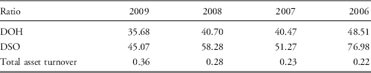
These ratios indicate that the company has improved on all three measures of activity over the four-year period. The company appears to be managing its inventory more efficiently, is collecting receivables faster, and is generating a higher level of revenues relative to total assets. The overall trend appears good, but thus far, the analyst has only determined what happened. A more important question is why the ratios improved, because understanding good changes as well as bad ones facilitates judgments about the company’s future performance. To answer this question, the analyst examines company financial reports as well as external information about the industry and economy. In examining the annual report, the analyst notes that in the fourth quarter of 2009, the company experienced an “inventory correction” and that the company recorded an allowance for the decline in market value and obsolescence of inventory of about 15 percent of year-end inventory value (compared with about a 6 percent allowance in the prior year). This reduction in the value of inventory accounts for a large portion of the decline in DOH from 40.70 in 2008 to 35.68 in 2009. Management claims that this inventory obsolescence is a short-term issue; analysts can watch DOH in future interim periods to confirm this assertion. In any event, all else being equal, the analyst would likely expect DOH to return to a level closer to 40 days going forward.
More positive interpretations can be drawn from the total asset turnover. The analyst finds that the company’s revenues increased more than 35 percent while total assets only increased by about 6 percent. Based on external information about the industry and economy, the analyst attributes the increased revenues both to overall growth in the industry and to the company’s increased market share. Management was able to achieve growth in revenues with a comparatively modest increase in assets, leading to an improvement in total asset turnover. Note further that part of the reason for the increase in asset turnover is lower DOH and DSO.
4.3. Liquidity Ratios
Liquidity analysis, which focuses on cash flows, measures a company’s ability to meet its short-term obligations. Liquidity measures how quickly assets are converted into cash. Liquidity ratios also measure the ability to pay off short-term obligations. In day-to-day operations, liquidity management is typically achieved through efficient use of assets. In the medium term, liquidity in the nonfinancial sector is also addressed by managing the structure of liabilities. (See the discussion on financial sector later.)
The level of liquidity needed differs from one industry to another. A particular company’s liquidity position may vary according to the anticipated need for funds at any given time. Judging whether a company has adequate liquidity requires analysis of its historical funding requirements, current liquidity position, anticipated future funding needs, and options for reducing funding needs or attracting additional funds (including actual and potential sources of such funding).
Larger companies are usually better able to control the level and composition of their liabilities than smaller companies. Therefore, they may have more potential funding sources, including public capital and money markets. Greater discretionary access to capital markets also reduces the size of the liquidity buffer needed relative to companies without such access.
Contingent liabilities, such as letters of credit or financial guarantees, can also be relevant when assessing liquidity. The importance of contingent liabilities varies for the nonbanking and banking sector. In the nonbanking sector, contingent liabilities (usually disclosed in the footnotes to the company’s financial statements) represent potential cash outflows, and when appropriate, should be included in an assessment of a company’s liquidity. In the banking sector, contingent liabilities represent potentially significant cash outflows that are not dependent on the bank’s financial condition. Although outflows in normal market circumstances typically may be low, a general macroeconomic or market crisis can trigger a substantial increase in cash outflows related to contingent liabilities because of the increase in defaults and business bankruptcies that often accompany such events. In addition, such crises are usually characterized by diminished levels of overall liquidity, which can further exacerbate funding shortfalls. Therefore, for the banking sector, the effect of contingent liabilities on liquidity warrants particular attention.
4.3.1. Calculation of Liquidity Ratios
Common liquidity ratios are presented in Exhibit 7-12. These liquidity ratios reflect a company’s position at a point in time and, therefore, typically use data from the ending balance sheet rather than averages. The current, quick, and cash ratios reflect three measures of a company’s ability to pay current liabilities. Each uses a progressively stricter definition of liquid assets.
The defensive interval ratio measures how long a company can pay its daily cash expenditures using only its existing liquid assets, without additional cash flow coming in. This ratio is similar to the “burn rate” often computed for start-up Internet companies in the late 1990s or for biotechnology companies. The numerator of this ratio includes the same liquid assets used in the quick ratio, and the denominator is an estimate of daily cash expenditures. To obtain daily cash expenditures, the total of cash expenditures for the period is divided by the number of days in the period. Total cash expenditures for a period can be approximated by summing all expenses on the income statement—such as cost of goods sold; selling, general, and administrative expenses; and research and development expenses—and then subtracting any noncash expenses, such as depreciation and amortization. (Typically, taxes are not included.)
The cash conversion cycle, a financial metric not in ratio form, measures the length of time required for a company to go from cash paid (used in its operations) to cash received (as a result of its operations). The cash conversion cycle is sometimes expressed as the length of time funds are tied up in working capital. During this period of time, the company needs to finance its investment in operations through other sources (i.e., through debt or equity).
EXHIBIT 7-12 Definitions of Commonly Used Liquidity Ratios
| Liquidity Ratios | Numerator | Denominator |
| Current ratio | Current assets | Current liabilities |
| Quick ratio | Cash + Short-term marketable investments + Receivables | Current liabilities |
| Cash ratio | Cash + Short-term marketable investments | Current liabilities |
| Defensive interval ratio | Cash + Short-term marketable investments + Receivables | Daily cash expenditures |
| Additional Liquidity Measure | ||
| Cash conversion cycle (net operating cycle) | DOH + DSO − Number of days of payables | |
4.3.2. Interpretation of Liquidity Ratios
In the following, we discuss the interpretation of the five basic liquidity measures presented in Exhibit 7-12.
Current ratio. This ratio expresses current assets in relation to current liabilities. A higher ratio indicates a higher level of liquidity (i.e., a greater ability to meet short-term obligations). A current ratio of 1.0 would indicate that the book value of its current assets exactly equals the book value of its current liabilities.
A lower ratio indicates less liquidity, implying a greater reliance on operating cash flow and outside financing to meet short-term obligations. Liquidity affects the company’s capacity to take on debt. The current ratio implicitly assumes that inventories and accounts receivable are indeed liquid (which is presumably not the case when related turnover ratios are low).
Quick ratio. The quick ratio is more conservative than the current ratio because it includes only the more liquid current assets (sometimes referred to as “quick assets”) in relation to current liabilities. Like the current ratio, a higher quick ratio indicates greater liquidity.
The quick ratio reflects the fact that certain current assets—such as prepaid expenses, some taxes, and employee-related prepayments—represent costs of the current period that have been paid in advance and cannot usually be converted back into cash. This ratio also reflects the fact that inventory might not be easily and quickly converted into cash, and furthermore, that a company would probably not be able to sell all of its inventory for an amount equal to its carrying value, especially if it were required to sell the inventory quickly. In situations where inventories are illiquid (as indicated, for example, by low inventory turnover ratios), the quick ratio may be a better indicator of liquidity than is the current ratio.
Cash ratio. The cash ratio normally represents a reliable measure of an entity’s liquidity in a crisis situation. Only highly marketable short-term investments and cash are included. In a general market crisis, the fair value of marketable securities could decrease significantly as a result of market factors, in which case even this ratio might not provide reliable information.
Defensive interval ratio. This ratio measures how long the company can continue to pay its expenses from its existing liquid assets without receiving any additional cash inflow. A defensive interval ratio of 50 would indicate that the company can continue to pay its operating expenses for 50 days before running out of quick assets, assuming no additional cash inflows. A higher defensive interval ratio indicates greater liquidity. If a company’s defensive interval ratio is very low relative to peer companies or to the company’s own history, the analyst would want to ascertain whether there is sufficient cash inflow expected to mitigate the low defensive interval ratio.
Cash conversion cycle (net operating cycle). This metric indicates the amount of time that elapses from the point when a company invests in working capital until the point at which the company collects cash. In the typical course of events, a merchandising company acquires inventory on credit, incurring accounts payable. The company then sells that inventory on credit, increasing accounts receivable. Afterwards, it pays out cash to settle its accounts payable, and it collects cash in settlement of its accounts receivable. The time between the outlay of cash and the collection of cash is called the “cash conversion cycle.” A shorter cash conversion cycle indicates greater liquidity. A short cash conversion cycle implies that the company only needs to finance its inventory and accounts receivable for a short period of time. A longer cash conversion cycle indicates lower liquidity; it implies that the company must finance its inventory and accounts receivable for a longer period of time, possibly indicating a need for a higher level of capital to fund current assets. Example 7-9 demonstrates the advantages of a short cash conversion cycle as well as how a company’s business strategies are reflected in financial ratios.
EXAMPLE 7-9 Evaluation of Liquidity Measures
An analyst is evaluating the liquidity of Dell and finds that Dell’s 10-K provides a computation of the number of days of receivables, inventory, and accounts payable, as well as the overall cash conversion cycle, as follows:
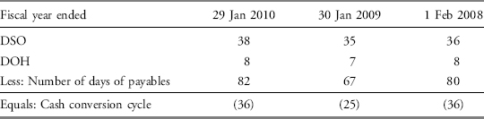
The minimal DOH indicates that Dell maintains lean inventories, which is attributable to key aspects of the company’s business model. The company does not build a computer until it is ordered and maintains a just-in-time approach to inventory management. In isolation, the increase in number of days payable (from 67 days in 2009 to 82 days in 2010) might suggest an inability to pay suppliers; however, in Dell’s case, the balance sheet indicates that the company has more than $10 billion of cash and short-term investments, which would be more than enough to pay suppliers sooner if Dell chose to do so. Instead, Dell takes advantage of the favorable credit terms granted by its suppliers. The overall effect is a negative cash cycle, a somewhat unusual result. Instead of requiring additional capital to fund working capital as is the case for most companies, Dell has excess cash to invest for about 37 days (reflected on the balance sheet as short-term investments) on which it is earning, rather than paying, interest.
For comparison, the analyst finds the cash conversion cycle reported in the annual reports of two of Dell’s competitors, Lenovo and Hewlett-Packard (NYSE: HPQ):
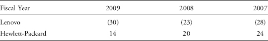
The analyst notes that of the three, only Hewlett-Packard has to raise capital for working capital purposes. While both Dell and Lenovo have consistently negative cash conversion cycles, Lenovo has been slightly less liquid than Dell, evidenced by its slightly less negative cash conversion cycle.
EXAMPLE 7-10 Bounds and Context of Financial Measures
The previous example focused on the cash conversion cycle, which many companies identify as a key performance metric. The less positive the number of days in the cash conversion cycle, typically, the better it is considered to be. However, is this always true?
This example considers the following question: If a larger negative number of days in a cash conversion cycle is considered to be a desirable performance metric, does identifying a company with a large negative cash conversion cycle necessarily imply good performance?
Using the Compustat database, the company identified as the U.S. computer technology company with the most negative number of days in its cash conversion cycle during the 2005 to 2009 period is National Datacomputer Inc. (OTC: NDCP), which had a negative cash conversion cycle of 275.5 days in 2008.
The reason for the negative cash conversion cycle is that the company’s accounts payable increased substantially over the period. An increase from approximately 66 days in 2005 to 295 days in 2008 to pay trade creditors is clearly a negative signal. In addition, the company’s inventories disappeared, most likely because the company did not have enough cash to purchase new inventory and was unable to get additional credit from its suppliers.
EXHIBIT 7-13 National Datacomputer Inc.($ millions)
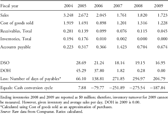
Of course, an analyst would have immediately noted the negative trends in these data, as well as additional data throughout the company’s financial statements. In its MD&A, the company clearly reports the risks as follows:
Because we have historically had losses and only a limited amount of cash has been generated from operations, we have funded our operating activities to date primarily from the sale of securities and from the sale of a product line in 2009. In order to continue to fund our operations, we may need to raise additional capital, through the sale of securities. We cannot be certain that any such financing will be available on acceptable terms, or at all. Moreover, additional equity financing, if available, would likely be dilutive to the holders of our common stock, and debt financing, if available, would likely involve restrictive covenants and a security interest in all or substantially all of our assets. If we fail to obtain acceptable financing when needed, we may not have sufficient resources to fund our normal operations which would have a material adverse effect on our business.
IF WE ARE UNABLE TO GENERATE ADEQUATE WORKING CAPITAL FROM OPERATIONS OR RAISE ADDITIONAL CAPITAL THERE IS SUBSTANTIAL DOUBT ABOUT THE COMPANY’S ABILITY TO CONTINUE AS A GOING CONCERN. (emphasis added by company)
Source: National Datacomputer Inc., 2009 Form 10-K, page 7.
In summary, it is always necessary to consider ratios within bounds of reasonability and to understand the reasons underlying changes in ratios. Ratios must not only be calculated but must also be interpreted by an analyst.
4.4. Solvency Ratios
Solvency refers to a company’s ability to fulfill its long-term debt obligations. Assessment of a company’s ability to pay its long-term obligations (i.e., to make interest and principal payments) generally includes an in-depth analysis of the components of its financial structure. Solvency ratios provide information regarding the relative amount of debt in the company’s capital structure and the adequacy of earnings and cash flow to cover interest expenses and other fixed charges (such as lease or rental payments) as they come due.
Analysts seek to understand a company’s use of debt for several main reasons. One reason is that the amount of debt in a company’s capital structure is important for assessing the company’s risk and return characteristics, specifically its financial leverage. Leverage is a magnifying effect that results from the use of fixed costs—costs that stay the same within some range of activity—and can take two forms: operating leverage and financial leverage.
Operating leverage results from the use of fixed costs in conducting the company’s business. Operating leverage magnifies the effect of changes in sales on operating income. Profitable companies may use operating leverage because when revenues increase, with operating leverage, their operating income increases at a faster rate. The explanation is that, although variable costs will rise proportionally with revenue, fixed costs will not.
When financing a company (i.e., raising capital for it), the use of debt constitutes financial leverage because interest payments are essentially fixed financing costs. As a result of interest payments, a given percent change in EBIT results in a larger percent change in earnings before taxes (EBT). Thus, financial leverage tends to magnify the effect of changes in EBIT on returns flowing to equity holders. Assuming that a company can earn more on funds than it pays in interest, the inclusion of some level of debt in a company’s capital structure may lower a company’s overall cost of capital and increase returns to equity holders. However, a higher level of debt in a company’s capital structure increases the risk of default and results in higher borrowing costs for the company to compensate lenders for assuming greater credit risk. Starting with Modigliani and Miller (1958, 1963), a substantial amount of research has focused on determining a company’s optimal capital structure and the subject remains an important one in corporate finance.
In analyzing financial statements, an analyst aims to understand levels and trends in a company’s use of financial leverage in relation to past practices and the practices of peer companies. Analysts also need to be aware of the relationship between operating leverage (results from the use of noncurrent assets with fixed costs) and financial leverage (results from the use of long-term debt with fixed costs). The greater a company’s operating leverage, the greater the risk of the operating income stream available to cover debt payments; operating leverage can thus limit a company’s capacity to use financial leverage.
A company’s relative solvency is fundamental to valuation of its debt securities and its creditworthiness. Finally, understanding a company’s use of debt can provide analysts with insight into the company’s future business prospects because management’s decisions about financing may signal their beliefs about a company’s future. For example, the issuance of long-term debt to repurchase common shares may indicate that management believes the market is underestimating the company’s prospects and that the shares are undervalued.
4.4.1. Calculation of Solvency Ratios
Solvency ratios are primarily of two types. Debt ratios, the first type, focus on the balance sheet and measure the amount of debt capital relative to equity capital. Coverage ratios, the second type, focus on the income statement and measure the ability of a company to cover its debt payments. These ratios are useful in assessing a company’s solvency and, therefore, in evaluating the quality of a company’s bonds and other debt obligations.
Exhibit 7-14 describes commonly used solvency ratios. The first three of the debt ratios presented use total debt in the numerator. The definition of total debt used in these ratios varies among informed analysts and financial data vendors, with some using the total of interest-bearing short-term and long-term debt, excluding liabilities such as accrued expenses and accounts payable. (For calculations in this chapter, we use this definition.) Other analysts use definitions that are more inclusive (e.g., all liabilities) or restrictive (e.g., long-term debt only, in which case the ratio is sometimes qualified as “long-term,” as in “long-term debt-to-equity ratio”). If using different definitions of total debt materially changes conclusions about a company’s solvency, the reasons for the discrepancies warrant further investigation.
EXHIBIT 7-14 Definitions of Commonly Used Solvency Ratios
| Solvency Ratios | Numerator | Denominator |
| Debt ratios | ||
| Debt-to-assets ratioa | Total debtb | Total assets |
| Debt-to-capital ratio | Total debtb | Total debtb + Total shareholders’ equity |
| Debt-to-equity ratio | Total debtb | Total shareholders’ equity |
| Financial leverage ratio | Average total assets | Average total equity |
| Coverage ratios | ||
| Interest coverage | EBIT | Interest payments |
| Fixed charge coverage | EBIT + Lease payments | Interest payments + Lease payments |
a“Total debt ratio” is another name sometimes used for this ratio.
bIn this chapter, we take total debt in this context to be the sum of interest-bearing short-term and long-term debt.
4.2.2. Interpretation of Solvency Ratios
In the following, we discuss the interpretation of the basic solvency ratios presented in Exhibit 7-14.
Debt-to-assets ratio. This ratio measures the percentage of total assets financed with debt. For example, a debt-to-assets ratio of 0.40 or 40 percent indicates that 40 percent of the company’s assets are financed with debt. Generally, higher debt means higher financial risk and thus weaker solvency.
Debt-to-capital ratio. The debt-to-capital ratio measures the percentage of a company’s capital (debt plus equity) represented by debt. As with the previous ratio, a higher ratio generally means higher financial risk and thus indicates weaker solvency.
Debt-to-equity ratio. The debt-to-equity ratio measures the amount of debt capital relative to equity capital. Interpretation is similar to the preceding two ratios (i.e., a higher ratio indicates weaker solvency). A ratio of 1.0 would indicate equal amounts of debt and equity, which is equivalent to a debt-to-capital ratio of 50 percent. Alternative definitions of this ratio use the market value of stockholders’ equity rather than its book value (or use the market values of both stockholders’ equity and debt).
Financial leverage ratio. This ratio (often called simply the “leverage ratio”) measures the amount of total assets supported for each one money unit of equity. For example, a value of 3 for this ratio means that each €1 of equity supports €3 of total assets. The higher the financial leverage ratio, the more leveraged the company is in the sense of using debt and other liabilities to finance assets. This ratio is often defined in terms of average total assets and average total equity and plays an important role in the DuPont decomposition of return on equity that will be presented in Section 4.6.2.
Interest coverage. This ratio measures the number of times a company’s EBIT could cover its interest payments. Thus, it is sometimes referred to as “times interest earned.” A higher interest coverage ratio indicates stronger solvency, offering greater assurance that the company can service its debt (i.e., bank debt, bonds, notes) from operating earnings.
Fixed charge coverage. This ratio relates fixed charges, or obligations, to the cash flow generated by the company. It measures the number of times a company’s earnings (before interest, taxes, and lease payments) can cover the company’s interest and lease payments.9 Similar to the interest coverage ratio, a higher fixed charge coverage ratio implies stronger solvency, offering greater assurance that the company can service its debt (i.e., bank debt, bonds, notes, and leases) from normal earnings. The ratio is sometimes used as an indication of the quality of the preferred dividend, with a higher ratio indicating a more secure preferred dividend.
Example 7-11 demonstrates the use of solvency ratios in evaluating the creditworthiness of a company.
EXAMPLE 7-11 Evaluation of Solvency Ratios
A credit analyst is evaluating the solvency of Alcatel-Lucent (Euronext Paris: ALU) as of the beginning of 2010. The following data are gathered from the company’s 2009 annual report (in € millions):
| 2009 | 2008 | |
| Total equity | 4,309 | 5,224 |
| Accrued pension | 5,043 | 4,807 |
| Long-term debt | 4,179 | 3,998 |
| Other long term liabilities* | 1,267 | 1,595 |
| Current liabilities* | 9,050 | 11,687 |
| Total equity+Liabilities (equals Total assets) | 23,848 | 27,311 |
*For purposes of this example, assume that these items are noninterest bearing, and that Long-term debt equals Total debt. In practice, an analyst could refer to Alcatel’s footnotes to confirm details, rather than making an assumption.
1. A. Calculate the company’s financial leverage ratio for 2009.
B. Interpret the financial leverage ratio calculated in Part A.
2. A. What are the company’s debt-to-assets, debt-to-capital, and debt-to-equity ratios for the two years?
B. Is there any discernable trend over the two years?
Solutions to 1. (Amounts are millions of euro.)
A. Average total assets was (27,311+23,848)/2=25,580 and average total equity was (5,224+4,309)/2=4,767. Thus, financial leverage was 25,580/4,767= 5.37.
B. For 2009, every €1 in total equity supported €5.37 in total assets, on average.
Solutions to 2. (Amounts are millions of euro.)
A. Debt-to-assets for 2008=3,998/27,311=14.64%
Debt-to-assets for 2009=4,179/23,848=17.52%
Debt-to-capital for 2008=3,998/(3,998+5,224)=43.35%
Debt-to-capital for 2009=4,179/(4,179+4,309)=49.23%
Debt-to-equity for 2008=3,998/5,224=0.77
Debt-to-equity for 2009=4,179/4,309=0.97
B. On all three metrics, the company’s leverage has increased. The increase in debt as part of the company’s capital structure indicates that the company’s solvency has weakened. From a creditor’s perspective, lower solvency (higher debt) indicates higher risk of default on obligations.
As with all ratio analysis, it is important to consider leverage ratios in a broader context. In general, companies with lower business risk and operations that generate steady cash flows are better positioned to take on more leverage without a commensurate increase in the risk of insolvency. In other words, a higher proportion of debt financing poses less risk of nonpayment of interest and debt principal to a company with steady cash flows than to a company with volatile cash flows.
4.5. Profitability Ratios
The ability to generate profit on capital invested is a key determinant of a company’s overall value and the value of the securities it issues. Consequently, many equity analysts would consider profitability to be a key focus of their analytical efforts.
Profitability reflects a company’s competitive position in the market, and by extension, the quality of its management. The income statement reveals the sources of earnings and the components of revenue and expenses. Earnings can be distributed to shareholders or reinvested in the company. Reinvested earnings enhance solvency and provide a cushion against short-term problems.
4.5.1. Calculation of Profitability Ratios
Profitability ratios measure the return earned by the company during a period. Exhibit 7-15 provides the definitions of a selection of commonly used profitability ratios. Return-on-sales profitability ratios express various subtotals on the income statement (e.g., gross profit, operating profit, net profit) as a percentage of revenue. Essentially, these ratios constitute part of a common-size income statement discussed earlier. Return on investment profitability ratios measure income relative to assets, equity, or total capital employed by the company. For operating ROA, returns are measured as operating income, i.e., prior to deducting interest on debt capital. For ROA and ROE, returns are measured as net income, i.e., after deducting interest paid on debt capital. For return on common equity, returns are measured as net income minus preferred dividends (because preferred dividends are a return to preferred equity).
EXHIBIT 7-15 Definitions of Commonly Used Profitability Ratios
| Profitability Ratios | Numerator | Denominator |
| Return on Sales10 | ||
| Gross profit margin | Gross profit | Revenue |
| Operating profit margin | Operating income11 | Revenue |
| Pretax margin | EBT (earnings before tax but after interest) | Revenue |
| Net profit margin | Net income | Revenue |
| Return on Investment | ||
| Operating ROA | Operating income | Average total assets |
| ROA | Net income | Average total assets |
| Return on total capital | EBIT | Short- and long-term debt and equity |
| ROE | Net income | Average total equity |
| Return on common equity | Net income − Preferred dividends | Average common equity |
4.5.2. Interpretation of Profitability Ratios
In the following, we discuss the interpretation of the profitability ratios presented in Exhibit 7-15. For each of the profitability ratios, a higher ratio indicates greater profitability.
Gross profit margin. Gross profit margin indicates the percentage of revenue available to cover operating and other expenses and to generate profit. Higher gross profit margin indicates some combination of higher product pricing and lower product costs. The ability to charge a higher price is constrained by competition, so gross profits are affected by (and usually inversely related to) competition. If a product has a competitive advantage (e.g., superior branding, better quality, or exclusive technology), the company is better able to charge more for it. On the cost side, higher gross profit margin can also indicate that a company has a competitive advantage in product costs.
Operating profit margin. Operating profit is calculated as gross profit minus operating costs. So, an operating profit margin increasing faster than the gross profit margin can indicate improvements in controlling operating costs, such as administrative overheads. In contrast, a declining operating profit margin could be an indicator of deteriorating control over operating costs.
Pretax margin. Pretax income (also called “earnings before tax” or “EBT”) is calculated as operating profit minus interest, and the pretax margin is the ratio of pretax income to revenue. The pretax margin reflects the effects on profitability of leverage and other (nonoperating) income and expenses. If a company’s pretax margin is increasing primarily as a result of increasing amounts of nonoperating income, the analyst should evaluate whether this increase reflects a deliberate change in a company’s business focus and, therefore, the likelihood that the increase will continue.
Net profit margin. Net profit, or net income, is calculated as revenue minus all expenses. Net income includes both recurring and nonrecurring components. Generally, the net income used in calculating the net profit margin is adjusted for nonrecurring items to offer a better view of a company’s potential future profitability.
ROA. ROA measures the return earned by a company on its assets. The higher the ratio, the more income is generated by a given level of assets. Most databases compute this ratio as:
![]()
An issue with this computation is that net income is the return to equity holders, whereas assets are financed by both equity holders and creditors. Interest expense (the return to creditors) has already been subtracted in the numerator. Some analysts, therefore, prefer to add back interest expense in the numerator. In such cases, interest must be adjusted for income taxes because net income is determined after taxes. With this adjustment, the ratio would be computed as:
![]()
Alternatively, some analysts elect to compute ROA on a pre-interest and pre-tax basis (operating ROA in Exhibit 7-15) as:
![]()
In this ROA calculation, returns are measured prior to deducting interest on debt capital (i.e., as operating income or EBIT). This measure reflects the return on all assets invested in the company, whether financed with liabilities, debt, or equity. Whichever form of ROA is chosen, the analyst must use it consistently in comparisons to other companies or time periods.
Return on total capital. Return on total capital measures the profits a company earns on all of the capital that it employs (short-term debt, long-term debt, and equity). As with operating ROA, returns are measured prior to deducting interest on debt capital (i.e., as operating income or EBIT).
ROE. ROE measures the return earned by a company on its equity capital, including minority equity, preferred equity, and common equity. As noted, return is measured as net income (i.e., interest on debt capital is not included in the return on equity capital). A variation of ROE is return on common equity, which measures the return earned by a company only on its common equity.
Both ROA and ROE are important measures of profitability and will be explored in more detail in section 4.6.2. As with other ratios, profitability ratios should be evaluated individually and as a group to gain an understanding of what is driving profitability (operating versus nonoperating activities). Example 7-12 demonstrates the evaluation of profitability ratios and the use of the management report (sometimes called management’s discussion and analysis or management commentary) that accompanies financial statements to explain the trend in ratios.
EXAMPLE 7-12 Evaluation of Profitability Ratios
An analyst is evaluating the profitability of Daimler AG (Xetra: DAI) over a recent five-year period. He gathers the following revenue data and calculates the following profitability ratios from information in Daimler’s annual reports:
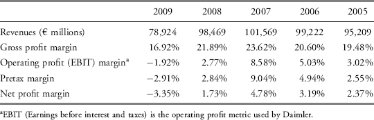
Daimler’s revenue declined from 2007 to 2008 and from 2008 to 2009. Further, Daimler’s 2009 revenues were the lowest of the five years. Management’s discussion of the decline in revenue and EBIT in the 2009 Annual Report notes the following:
The main reason for the decline [in EBIT] was a significant drop in revenue due to markedly lower unit sales in all vehicle segments as a result of the global economic downturn. Cost savings achieved through permanent and temporary cost reductions and efficiency improvements realized through ongoing optimization programs could only partially compensate for the drop in revenue.
1. Compare gross profit margins and operating profit margins over the 2005 to 2009 period.
2. Explain the decline in operating profit margin in 2009.
3. Explain why the pretax margin might have decreased to a greater extent than the operating profit margin in 2009.
4. Compare net profit margins and pretax margins over 2007 to 2009
Solution to 1: Gross profit margin improved from 2005 to 2007 as a result of some combination of price increases and/or cost control. However, gross profit margin declined from 2007 to 2009. Operating profit margin showed a similar trend. In 2009, the operating profit margin was negative.
Solution to 2: The decline in operating profit from 2.77 percent in 2008 to −1.92 percent in 2009 appears to be the result of Daimler’s operating leverage. Management indicated that revenue declined in 2009 and reductions in expenses were not enough to offset the revenue decline. Management tried to increase efficiency and reduce costs, including personnel expenses, but this did not sufficiently counteract the decrease in revenues. Expenses thus increased as a proportion of revenue, lowering the gross and operating profit margins. This is an example of the effects of operating leverage (fixed costs that could not be reduced) on profitability. In general, as revenue increases, to the extent that costs remain fixed, operating profit margins should increase. As revenue declines, the opposite occurs.
Solution to 3: Pretax margin was down substantially in 2009, indicating that the company may have had some nonoperating losses or high interest expense in that year. A review of the company’s annual report confirms that the cause was higher net interest expense. Specifically, the company increased financing liabilities, faced higher financing costs because of higher risk premiums on borrowing, and had lower interest income on investments. This is an example of the effects of financial leverage on profitability.
Solution to 4: Net profit margin followed the same pattern as pretax margin, increasing from 2005 to 2007 and then decreasing from 2007 to 2009. In the absence of major variation in the applicable tax rates, this would be expected as net profit margin is based on net income while pretax margin is based on EBT, and net income is EBT (1 − tax rate).
4.6. Integrated Financial Ratio Analysis
In prior sections, the text presented separately activity, liquidity, solvency, and profitability ratios. Prior to discussing valuation ratios, the following sections demonstrate the importance of examining a variety of financial ratios—not a single ratio or category of ratios in isolation—to ascertain the overall position and performance of a company. Experience shows that the information from one ratio category can be helpful in answering questions raised by another category and that the most accurate overall picture comes from integrating information from all sources. Section 4.6.1 provides some introductory examples of such analysis and Section 4.6.2 shows how return on equity can be analyzed into components related to profit margin, asset utilization (activity), and financial leverage.
4.6.1. The Overall Ratio Picture: Examples
This section presents two simple illustrations to introduce the use of a variety of ratios to address an analytical task. Example 7-13 shows how the analysis of a pair of activity ratios resolves an issue concerning a company’s liquidity. Example 7-14 shows that examining the overall ratios of multiple companies can assist an analyst in drawing conclusions about their relative performances.
EXAMPLE 7-13 A Variety of Ratios
An analyst is evaluating the liquidity of a Canadian manufacturing company and obtains the following liquidity ratios:
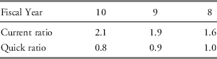
The ratios present a contradictory picture of the company’s liquidity. Based on the increase in its current ratio from 1.6 to 2.1, the company appears to have strong and improving liquidity; however, based on the decline of the quick ratio from 1.0 to 0.8, its liquidity appears to be deteriorating. Because both ratios have exactly the same denominator, current liabilities, the difference must be the result of changes in some asset that is included in the current ratio but not in the quick ratio (e.g., inventories). The analyst collects the following activity ratios:
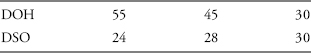
The company’s DOH has deteriorated from 30 days to 55 days, meaning that the company is holding increasingly larger amounts of inventory relative to sales. The decrease in DSO implies that the company is collecting receivables faster. If the proceeds from these collections were held as cash, there would be no effect on either the current ratio or the quick ratio. However, if the proceeds from the collections were used to purchase inventory, there would be no effect on the current ratio and a decline in the quick ratio (i.e., the pattern shown in this example). Collectively, the ratios suggest that liquidity is declining and that the company may have an inventory problem that needs to be addressed.
EXAMPLE 7-14 A Comparison of Two Companies (1)
An analyst collects the information12 shown in Exhibit 7-16 for two companies:
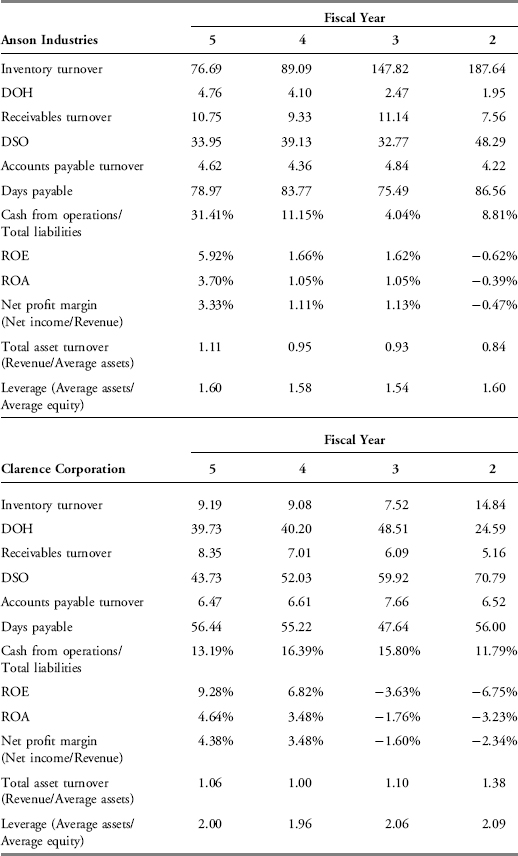
Which of the following choices best describes reasonable conclusions an analyst might make about the companies’ efficiency?
A. Over the past four years, Anson has shown greater improvement in efficiency than Clarence, as indicated by its total asset turnover ratio increasing from 0.84 to 1.11.
B. In FY5, Anson’s DOH of only 4.76 indicated that it was less efficient at inventory management than Clarence, which had DOH of 39.73.
C. In FY5, Clarence’s receivables turnover of 8.35 times indicated that it was more efficient at receivables management than Anson, which had receivables turnover of 10.75.
Solution: A is correct. Over the past four years, Anson has shown greater improvement in efficiency than Clarence, as indicated by its total asset turnover ratio increasing from 0.84 to 1.11. Over the same period of time, Clarence’s total asset turnover ratio has declined from 1.38 to 1.06. Choices B and C are incorrect because DOH and receivables turnover are misinterpreted.
4.6.2. DuPont Analysis: The Decomposition of ROE
As noted earlier, ROE measures the return a company generates on its equity capital. To understand what drives a company’s ROE, a useful technique is to decompose ROE into its component parts. (Decomposition of ROE is sometimes referred to as DuPont analysis because it was developed originally at that company.) Decomposing ROE involves expressing the basic ratio (i.e., net income divided by average shareholders’ equity) as the product of component ratios. Because each of these component ratios is an indicator of a distinct aspect of a company’s performance that affects ROE, the decomposition allows us to evaluate how these different aspects of performance affected the company’s profitability as measured by ROE.13
Decomposing ROE is useful in determining the reasons for changes in ROE over time for a given company and for differences in ROE for different companies in a given time period. The information gained can also be used by management to determine which areas they should focus on to improve ROE. This decomposition will also show why a company’s overall profitability, measured by ROE, is a function of its efficiency, operating profitability, taxes, and use of financial leverage. DuPont analysis shows the relationship between the various categories of ratios discussed in this chapter and how they all influence the return to the investment of the owners.
Analysts have developed several different methods of decomposing ROE. The decomposition presented here is one of the most commonly used and the one found in popular research databases, such as Bloomberg. Return on equity is calculated as:
![]()
The decomposition of ROE makes use of simple algebra and illustrates the relationship between ROE and ROA. Expressing ROE as a product of only two of its components, we can write:
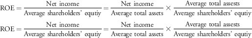
which can be interpreted as:
![]()
In other words, ROE is a function of a company’s ROA and its use of financial leverage (“leverage” for short, in this discussion). A company can improve its ROE by improving ROA or making more effective use of leverage. Consistent with the definition given earlier, leverage is measured as average total assets divided by average shareholders’ equity. If a company had no leverage (no liabilities), its leverage ratio would equal 1.0 and ROE would exactly equal ROA. As a company takes on liabilities, its leverage increases. As long as a company is able to borrow at a rate lower than the marginal rate it can earn investing the borrowed money in its business, the company is making an effective use of leverage and ROE would increase as leverage increases. If a company’s borrowing cost exceeds the marginal rate it can earn on investing in the business, ROE would decline as leverage increased because the effect of borrowing would be to depress ROA.
Using the data from Example 7-14 for Anson Industries, an analyst can examine the trend in ROE and determine whether the increase from an ROE of −0.625 percent in FY2 to 5.925 percent in FY5 is a function of ROA or the use of leverage:
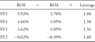
Over the four-year period, the company’s leverage factor was relatively stable. The primary reason for the increase in ROE is the increase in profitability measured by ROA.
Just as ROE can be decomposed, the individual components such as ROA can be decomposed. Further decomposing ROA, we can express ROE as a product of three component ratios:
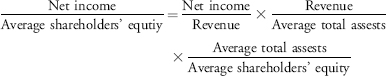
which can be interpreted as:
![]()
The first term on the right-hand side of this equation is the net profit margin, an indicator of profitability: how much income a company derives per one monetary unit (e.g., euro or dollar) of sales. The second term on the right is the asset turnover ratio, an indicator of efficiency: how much revenue a company generates per one money unit of assets. Note that ROA is decomposed into these two components: net profit margin and total asset turnover. A company’s ROA is a function of profitability (net profit margin) and efficiency (total asset turnover). The third term on the right-hand side of Equation 7.1b is a measure of financial leverage, an indicator of solvency: the total amount of a company’s assets relative to its equity capital. This decomposition illustrates that a company’s ROE is a function of its net profit margin, its efficiency, and its leverage. Again, using the data from Example 7-14 for Anson Industries, the analyst can evaluate in more detail the reasons behind the trend in ROE:14
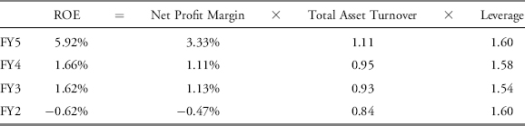
This further decomposition confirms that increases in profitability (measured here as net profit margin) are indeed an important contributor to the increase in ROE over the four-year period. However, Anson’s asset turnover has also increased steadily. The increase in ROE is, therefore, a function of improving profitability and improving efficiency. As noted previously, ROE decomposition can also be used to compare the ROEs of peer companies, as demonstrated in Example 7-15.
EXAMPLE 7-15 A Comparison of Two Companies (2)
Referring to the data for Anson Industries and Clarence Corporation in Example 7-14, which of the following choices best describes reasonable conclusions an analyst might make about the companies’ ROE?
A. Anson’s inventory turnover of 76.69 indicates it is more profitable than Clarence.
B. The main driver of Clarence’s superior ROE in FY5 is its more efficient use of assets.
C. The main drivers of Clarence’s superior ROE in FY5 are its greater use of debt financing and higher net profit margin.
Solution: C is correct. The main driver of Clarence’s superior ROE (9.28 percent compared with only 5.92 percent for Anson) in FY5 is its greater use of debt financing (leverage of 2.00 compared with Anson’s leverage of 1.60) and higher net profit margin (4.38 percent compared with only 3.33 percent for Anson). A is incorrect because inventory turnover is not a direct indicator of profitability. An increase in inventory turnover may indicate more efficient use of inventory, which in turn could affect profitability; however, an increase in inventory turnover would also be observed if a company was selling more goods even if it was not selling those goods at a profit. B is incorrect because Clarence has less efficient use of assets than Anson, indicated by turnover of 1.06 for Clarence compared with Anson’s turnover of 1.11.
To separate the effects of taxes and interest, we can further decompose the net profit margin and write:
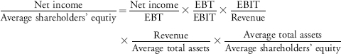
which can be interpreted as:
ROE = Tax burden × Interest burden × EBIT margin × Total assest turnover × Leverage
This five-way decomposition is the one found in financial databases such as Bloomberg. The first term on the right-hand side of this equation measures the effect of taxes on ROE. Essentially, it reflects one minus the average tax rate, or how much of a company’s pretax profits it gets to keep. This can be expressed in decimal or percentage form. So, a 30 percent tax rate would yield a factor of 0.70 or 70 percent. A higher value for the tax burden implies that the company can keep a higher percentage of its pretax profits, indicating a lower tax rate. A decrease in the tax burden ratio implies the opposite (i.e., a higher tax rate leaving the company with less of its pretax profits).
The second term on the right-hand side captures the effect of interest on ROE. Higher borrowing costs reduce ROE. Some analysts prefer to use operating income instead of EBIT for this term and the following term. Either operating income or EBIT is acceptable as long as it is applied consistently. In such a case, the second term would measure both the effect of interest expense and nonoperating income on ROE.
The third term on the right-hand side captures the effect of operating margin (if operating income is used in the numerator) or EBIT margin (if EBIT is used) on ROE. In either case, this term primarily measures the effect of operating profitability on ROE.
The fourth term on the right-hand side is again the total asset turnover ratio, an indicator of the overall efficiency of the company (i.e., how much revenue it generates per unit of total assets). The fifth term on the right-hand side is the financial leverage ratio described earlier—the total amount of a company’s assets relative to its equity capital.
This decomposition expresses a company’s ROE as a function of its tax rate, interest burden, operating profitability, efficiency, and leverage. An analyst can use this framework to determine what factors are driving a company’s ROE. The decomposition of ROE can also be useful in forecasting ROE based upon expected efficiency, profitability, financing activities, and tax rates. The relationship of the individual factors, such as ROA to the overall ROE, can also be expressed in the form of an ROE tree to study the contribution of each of the five factors, as shown in Exhibit 7-17 for Anson Industries.15
Exhibit 7-17 shows that Anson’s ROE of 5.92 percent in FY5 can be decomposed into ROA of 3.70 percent and leverage of 1.60. ROA can further be decomposed into a net profit margin of 3.33 percent and total asset turnover of 1.11. Net profit margin can be decomposed into a tax burden of 0.70 (an average tax rate of 30 percent), an interest burden of 0.90, and an EBIT margin of 5.29 percent. Overall ROE is decomposed into five components.
EXHIBIT 7-17 DuPont Analysis of Anson Industries’ ROE: Fiscal Year 5
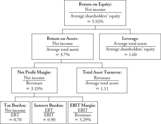
Example 7-16 demonstrates how the five-component decomposition can be used to determine reasons behind the trend in a company’s ROE.
The most detailed decomposition of ROE that we have presented is a five-way decomposition. Nevertheless, an analyst could further decompose individual components of a five-way analysis. For example, EBIT margin (EBIT/Revenue) could be further decomposed into a nonoperating component (EBIT/Operating income) and an operating component (Operating income/Revenue). The analyst can also examine which other factors contributed to these five components. For example, an improvement in efficiency (total asset turnover) may have resulted from better management of inventory (DOH) or better collection of receivables (DSO).
EXAMPLE 7-16 Five-Way Decomposition of ROE
An analyst examining Royal Dutch Shell PLC (Amsterdam and London SEs: RDSA) wishes to understand the factors driving the trend in ROE over a recent four-year period. The analyst obtains and calculates the following data from Shell’s annual reports:
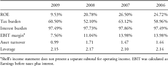
What might the analyst conclude?
Solution: The tax burden measure has varied, with no obvious trend. In the most recent year, 2009, taxes declined as a percentage of pretax profit. (Because the tax burden reflects the relation of after-tax profits to pretax profits, the increase from 52.10 percent in 2008 to 60.50 percent in 2009 indicates that taxes declined as a percentage of pretax profits.) This decline in average tax rates could be a result of lower tax rates from new legislation or revenue in a lower tax jurisdiction. The interest burden has remained fairly constant over the four-year period indicating that the company maintains a fairly constant capital structure. Operating margin (EBIT margin) declined over the period, indicating the company’s operations were less profitable. This decline is generally consistent with declines in oil prices in 2009 and declines in refining industry gross margins in 2008 and 2009. The company’s efficiency (asset turnover) decreased in 2009. The company’s leverage remained constant, consistent with the constant interest burden. Overall, the trend in ROE (declining substantially over the recent years) resulted from decreases in operating profits and a lower asset turnover. Additional research on the causes of these changes is required in order to develop expectations about the company’s future performance.
One application of financial analysis is to select securities as part of the equity portfolio management process. Analysts are interested in valuing a security to assess its merits for inclusion or retention in a portfolio. The valuation process has several steps, including:16
1. Understanding the business and the existing financial profile.
2. Forecasting company performance.
3. Selecting the appropriate valuation model.
4. Converting forecasts to a valuation.
5. Making the investment decision.
Financial analysis assists in providing the core information to complete the first two steps of this valuation process: understanding the business and forecasting performance.
Fundamental equity analysis involves evaluating a company’s performance and valuing its equity in order to assess its relative attractiveness as an investment. Analysts use a variety of methods to value a company’s equity, including valuation ratios (e.g., the price-to-earnings or P/E ratio), discounted cash flow approaches, and residual income approaches (ROE compared with the cost of capital), among others. The following section addresses the first of these approaches—the use of valuation ratios.
5.1. Valuation Ratios
Valuation ratios have long been used in investment decision making. A well known example is the price to earnings ratio (P/E ratio)—probably the most widely cited indicator in discussing the value of equity securities—which relates share price to the earnings per share (EPS). Additionally, some analysts use other market multiples, such as price to book value (P/B) and price to cash flow (P/CF). The following sections explore valuation ratios and other quantities related to valuing equities.
5.1.1. Calculation of Valuation Ratios and Related Quantities
Exhibit 7-18 describes the calculation of some common valuation ratios and related quantities.
EXHIBIT 7-18 Definitions of Selected Valuation Ratios and Related Quantities
| Numerator | Denominator | |
| Valuation ratios | ||
| P/E | Price per share | Earnings per share |
| P/CF | Price per share | Cash flow per share |
| P/S | Price per share | Sales per share |
| P/BV | Price per share | Book value per share |
| Per-share quantities | ||
| Basic EPS | Net income minus preferred dividends | Weighted average number of ordinary shares outstanding |
| Diluted EPS | Adjusted income available for ordinary shares, reflecting conversion of dilutive securities | Weighted average number of ordinary and potential ordinary shares outstanding |
| Cash flow per share | Cash flow from operations | Weighted average number of shares outstanding |
| EBITDA per share | EBITDA | Weighted average number of shares outstanding |
| Dividends per share | Common dividends declared | Weighted average number of ordinary shares outstanding |
| Dividend-related quantities | ||
| Dividend payout ratio | Common share dividends | Net income attributable to common shares |
| Retention rate (b) | Net income attributable to common shares − Common share dividends | Net income attributable to common shares |
| Sustainable growth rate | b × ROE |
The P/E ratio expresses the relationship between the price per share and the amount of earnings attributable to a single share. In other words, the P/E ratio tells us how much an investor in common stock pays per dollar of earnings.
Because P/E ratios are calculated using net income, the ratios can be sensitive to nonrecurring earnings or one-time earnings events. In addition, because net income is generally considered to be more susceptible to manipulation than are cash flows, analysts may use price to cash flow as an alternative measure—particularly in situations where earnings quality may be an issue. EBITDA per share, because it is calculated using income before interest, taxes, and depreciation, can be used to eliminate the effect of different levels of fixed asset investment across companies. It facilitates comparison between companies in the same sector but at different stages of infrastructure maturity. Price to sales is calculated in a similar manner and is sometimes used as a comparative price metric when a company does not have positive net income.
Another price-based ratio that facilitates useful comparisons of companies’ stock prices is price to book value, or P/B, which is the ratio of price to book value per share. This ratio is often interpreted as an indicator of market judgment about the relationship between a company’s required rate of return and its actual rate of return. Assuming that book values reflect the fair values of the assets, a price to book ratio of one can be interpreted as an indicator that the company’s future returns are expected to be exactly equal to the returns required by the market. A ratio greater than one would indicate that the future profitability of the company is expected to exceed the required rate of return, and values of this ratio less than one indicate that the company is not expected to earn excess returns.
5.1.2. Interpretation of Earnings per Share
Exhibit 7-18 presented a number of per-share quantities that can be used in valuation ratios. In this section, we discuss the interpretation of one such critical quantity, earnings per share or EPS.17
EPS is simply the amount of earnings attributable to each share of common stock. In isolation, EPS does not provide adequate information for comparison of one company with another. For example, assume that two companies have only common stock outstanding and no dilutive securities outstanding. In addition, assume the two companies have identical net income of $10 million, identical book equity of $100 million and, therefore, identical profitability (10 percent, using ending equity in this case for simplicity). Furthermore, assume that Company A has 100 million weighted average common shares outstanding, whereas Company B has 10 million weighted average common shares outstanding. So, Company A will report EPS of $0.10 per share, and Company B will report EPS of $1 per share. The difference in EPS does not reflect a difference in profitability—the companies have identical profits and profitability. The difference reflects only a different number of common shares outstanding. Analysts should understand in detail the types of EPS information that companies report:
Basic EPS provides information regarding the earnings attributable to each share of common stock.18 To calculate basic EPS, the weighted average number of shares outstanding during the period is first calculated. The weighted average number of shares consists of the number of ordinary shares outstanding at the beginning of the period, adjusted by those bought back or issued during the period, multiplied by a time-weighting factor.
Accounting standards generally require the disclosure of basic as well as diluted EPS (diluted EPS includes the effect of all the company’s securities whose conversion or exercise would result in a reduction of basic EPS; dilutive securities include convertible debt, convertible preferred, warrants, and options). Basic EPS and diluted EPS must be shown with equal prominence on the face of the income statement for each class of ordinary share. Disclosure includes the amounts used as the numerators in calculating basic and diluted EPS, and a reconciliation of those amounts to the company’s profit or loss for the period. Because both basic and diluted EPS are presented in a company’s financial statements, an analyst does not need to calculate these measures for reported financial statements. Understanding the calculations is, however, helpful for situations requiring an analyst to calculate expected future EPS.
To calculate diluted EPS, earnings are adjusted for the after-tax effects assuming conversion, and the following adjustments are made to the weighted number of shares:
- The weighted average number of shares for basic EPS, plus those that would be issued on conversion of all dilutive potential ordinary shares. Potential ordinary shares are treated as dilutive when their conversion would decrease net profit per share from continuing ordinary operations.
- These shares are deemed to have been converted into ordinary shares at the beginning of the period or, if later, at the date of the issue of the shares.
- Options, warrants (and their equivalents), convertible instruments, contingently issuable shares, contracts that can be settled in ordinary shares or cash, purchased options, and written put options should be considered.
5.1.3. Dividend-Related Quantities
In this section, we discuss the interpretation of the dividend-related quantities presented in Exhibit 7-18. These quantities play a role in some present value models for valuing equities.
Dividend payout ratio. The dividend payout ratio measures the percentage of earnings that the company pays out as dividends to shareholders. The amount of dividends per share tends to be relatively fixed because any reduction in dividends has been shown to result in a disproportionately large reduction in share price. Because dividend amounts are relatively fixed, the dividend payout ratio tends to fluctuate with earnings. Therefore, conclusions about a company’s dividend payout policies should be based on examination of payout over a number of periods. Optimal dividend policy, similar to optimal capital structure, has been examined in academic research and continues to be a topic of significant interest in corporate finance.
Retention rate. The retention rate, or earnings retention rate, is the complement of the payout ratio or dividend payout ratio (i.e., 1 − payout ratio). Whereas the payout ratio measures the percentage of earnings that a company pays out as dividends, the retention rate is the percentage of earnings that a company retains. (Note that both the payout ratio and retention rate are both percentages of earnings. The difference in terminology—“ratio” versus “rate” versus “percentage”—reflects common usage rather than any substantive differences.)
Sustainable growth rate. A company’s sustainable growth rate is viewed as a function of its profitability (measured as ROE) and its ability to finance itself from internally generated funds (measured as the retention rate). The sustainable growth rate is ROE times the retention rate. A higher ROE and a higher retention rate result in a higher sustainable growth rate. This calculation can be used to estimate a company’s growth rate, a factor commonly used in equity valuation.
5.2. Industry-Specific Ratios
As stated earlier in this chapter, a universally accepted definition and classification of ratios does not exist. The purpose of ratios is to serve as indicators of important aspects of a company’s performance and value. Aspects of performance that are considered important in one industry may be irrelevant in another, and industry-specific ratios reflect these differences. For example, companies in the retail industry may report same-store sales changes because, in the retail industry, it is important to distinguish between growth that results from opening new stores and growth that results from generating more sales at existing stores. Industry-specific metrics can be especially important to the value of equity in early stage industries, where companies are not yet profitable.
In addition, regulated industries—especially in the financial sector—often are required to comply with specific regulatory ratios. For example, the banking sector’s liquidity and cash reserve ratios provide an indication of banking liquidity and reflect monetary and regulatory requirements. Banking capital adequacy requirements attempt to relate banks’ solvency requirements directly to their specific levels of risk exposure.
Exhibit 7-19 presents, for illustrative purposes only, some industry-specific and task-specific ratios.19
EXHIBIT 7-19 Definitions of Some Common Industry- and Task-Specific Ratios
| Ratio | Numerator | Denominator |
| Business risk | ||
| Coefficient of variation of operating income | Standard deviation of operating income | Average operating income |
| Coefficient of variation of net income | Standard deviation of net income | Average net income |
| Coefficient of variation of revenues | Standard deviation of revenue | Average revenue |
| Financial sector ratios | ||
| Capital adequacy—banks | Various components of capital | Various measures such as risk-weighted assets, market risk exposure, or level of operational risk assumed |
| Monetary reserve requirement (Cash reserve ratio) | Reserves held at central bank | Specified deposit liabilities |
| Liquid asset requirement | Approved “readily marketable” securities | Specified deposit liabilities |
| Net interest margin | Net interest income | Total interest-earning assets |
| Retail ratios | ||
| Same (or comparable) store sales | Average revenue growth year over year for stores open in both periods | Not applicable |
| Sales per square meter (or square foot) | Revenue | Total retail space in square meters (or square feet) |
| Service companies | ||
| Revenue per employee | Revenue | Total number of employees |
| Net income per employee | Net income | Total number of employees |
| Hotel | ||
| Average daily rate | Room revenue | Number of rooms sold |
| Occupancy rate | Number of rooms sold | Number of rooms available |
5.3. Research on Ratios in Equity Analysis
Some ratios may be particularly useful in equity analysis. The end product of equity analysis is often a valuation and investment recommendation. Theoretical valuation models are useful in selecting ratios that would be useful in this process. For example, a company’s P/B is theoretically linked to ROE, growth, and the required return. ROE is also a primary determinant of residual income in a residual income valuation model. In both cases, higher ROE relative to the required return denotes a higher valuation. Similarly, profit margin is related to justified price-to-sales (P/S) ratios. Another common valuation method involves forecasts of future cash flows that are discounted back to the present. Trends in ratios can be useful in forecasting future earnings and cash flows (e.g., trends in operating profit margin and collection of customer receivables). Future growth expectations are a key component of all of these valuation models. Trends may be useful in assessing growth prospects (when used in conjunction with overall economic and industry trends). The variability in ratios and common-size data can be useful in assessing risk, an important component of the required rate of return in valuation models. A great deal of academic research has focused on the use of these fundamental ratios in evaluating equity investments.
A classic study, Ou and Penman (1989a and 1989b), found that ratios and common-size metrics generated from accounting data were useful in forecasting earnings and stock returns. Ou and Penman examined 68 such metrics and found that these could be reduced to a more parsimonious list of relevant variables, including percentage changes in a variety of measures such as current ratio, inventory, and sales; gross and pretax margins; and returns on assets and equity. These variables were found to be useful in forecasting earnings and stock returns.
Subsequent studies have also demonstrated the usefulness of ratios in evaluation of equity investments and valuation. Lev and Thiagarajan (1993) examined fundamental financial variables used by analysts to assess whether they are useful in security valuation. They found that fundamental variables add about 70 percent to the explanatory power of earnings alone in predicting excess returns (stock returns in excess of those expected). The fundamental variables they found useful included percentage changes in inventory and receivables relative to sales, gross margin, sales per employee, and the change in bad debts relative to the change in accounts receivable, among others. Abarbanell and Bushee (1997) found some of the same variables useful in predicting future accounting earnings. Abarbanell and Bushee (1998) devised an investment strategy using these same variables and found that they can generate excess returns under this strategy.
Piotroski (2000) used financial ratios to supplement a value investing strategy and found that he can generate significant excess returns. Variables used by Piotroski include ROA, cash flow ROA, change in ROA, change in leverage, change in liquidity, change in gross margin, and change in inventory turnover.
This research shows that in addition to being useful in evaluating the past performance of a company, ratios can be useful in predicting future earnings and equity returns.
Credit risk is the risk of loss caused by a counterparty’s or debtor’s failure to make a promised payment. For example, credit risk with respect to a bond is the risk that the obligor (the issuer of the bond) is not able to pay interest and principal according to the terms of the bond indenture (contract). Credit analysis is the evaluation of credit risk.
Approaches to credit analysis vary and, as with all financial analysis, depend on the purpose of the analysis and the context in which it is done. Credit analysis for specific types of debt (e.g., acquisition financing and other highly leveraged financing) often involves projections of period-by-period cash flows similar to projections made by equity analysts. Whereas the equity analyst may discount projected cash flows to determine the value of the company’s equity, a credit analyst would use the projected cash flows to assess the likelihood of a company complying with its financial covenants in each period and paying interest and principal as due.20 The analysis would also include expectations about asset sales and refinancing options open to the company.
Credit analysis may relate to the borrower’s credit risk in a particular transaction or to its overall creditworthiness. In assessing overall creditworthiness, one general approach is credit scoring, a statistical analysis of the determinants of credit default.
Another general approach to credit analysis is the credit rating process that is used, for example, by credit rating agencies to assess and communicate the probability of default by an issuer on its debt obligations (e.g., commercial paper, notes, and bonds). A credit rating can be either long term or short term and is an indication of the rating agency’s opinion of the creditworthiness of a debt issuer with respect to a specific debt security or other obligation. Where a company has no debt outstanding, a rating agency can also provide an issuer credit rating that expresses an opinion of the issuer’s overall capacity and willingness to meet its financial obligations. The following sections review research on the use of ratios in credit analysis and the ratios commonly used in credit analysis.
6.1. The Credit Rating Process
The rating process involves both the analysis of a company’s financial reports as well as a broad assessment of a company’s operations. The credit evaluation process by any analyst includes many of the following procedures performed by analysts at credit rating agencies:21
- Meeting with management, typically including the chief financial officer, to discuss, for example, industry outlook, overview of major business segments, financial policies and goals, distinctive accounting practices, capital spending plans, and financial contingency plans.
- Tours of major facilities, time permitting.
- Meeting of a ratings committee where the analyst’s recommendations are voted on, after considering factors that include:
- Business risk, including the evaluation of:
- Operating environment.
- Industry characteristics (e.g., cyclicality and capital intensity).
- Success factors and areas of vulnerability.
- Company’s competitive position, including size and diversification.
- Financial risk, including
- The evaluation of capital structure, interest coverage, and profitability using ratio analysis.
- The examination of debt covenants.
- Evaluation of management
- Monitoring of publicly distributed ratings—including reconsideration of ratings due to changing conditions.
- Business risk, including the evaluation of:
In assigning credit ratings, rating agencies emphasize the importance of the relationship between a company’s business risk profile and its financial risk. “The company’s business risk profile determines the level of financial risk appropriate for any rating category.”22
When analyzing financial ratios, rating agencies normally investigate deviations of ratios from the median ratios of the universe of companies for which such ratios have been calculated and also use the median ratings as an indicator for the ratings grade given to a specific debt issuer. This so-called universe of rated companies changes constantly, and any calculations are obviously affected by economic factors as well as by mergers and acquisitions. International ratings include the influence of country and economic risk factors. Exhibit 7-20 presents key financial ratios used by Standard & Poor’s in evaluating industrial companies. Note that before calculating ratios, rating agencies make certain adjustments to reported financials such as adjusting debt to include off-balance sheet debt in a company’s total debt.
EXHIBIT 7-20 Selected Credit Ratios Used by Standard & Poor’s
| Credit Ratio | Numeratorb | Denominatorc |
| EBIT interest coverage | EBIT | Gross interest (prior to deductions for capitalized interest or interest income) |
| EBITDA interest coverage | EBITDA | Gross interest (prior to deductions for capitalized interest or interest income) |
| FFOa (Funds from operations) interest coverage | FFO plus interest paid, minus operating lease adjustments | Gross interest (prior to deductions for capitalized interest or interest income) |
| Return on capital | EBIT | Average capital, where capital=equity, plus noncurrent deferred taxes, plus debt |
| FFO (Funds from operations) to debt | FFO | Total debt |
| Free operating cash flow to debt | CFO (adjusted) minus capital expenditures | Total debt |
| Discretionary cash flow to debt | CFO minus capital expenditures minus dividends paid | Total debt |
| Net cash flow to capital expenditures | FFO minus dividends | Capital expenditures |
| Debt to EBITDA | Total debt | EBITDA |
| Total debt to total debt plus equity | Total debt | Total debt plus equity |
aFFO=funds from operations, defined as net income adjusted for noncash items; CFO = cash flow from operations.
bEmphasis is on earnings from continuing operations.
cNote that both the numerator and denominator definitions are adjusted from ratio to ratio and may not correspond to the definitions used elsewhere in this chapter.
Source: Based on data from Standard & Poor’s Corporate Ratings Criteria (2008), p. 52.
6.2. Research on Ratios in Credit Analysis
A great deal of academic and practitioner research has focused on determining which ratios are useful in assessing the credit risk of a company, including the risk of bankruptcy.
One of the earliest studies examined individual ratios to assess their ability to predict failure of a company up to five years in advance. Beaver (1967) found that six ratios could correctly predict company failure one year in advance 90 percent of the time and five years in advance at least 65 percent of the time. The ratios found effective by Beaver were cash flow to total debt, ROA, total debt to total assets, working capital to total assets, the current ratio, and the no-credit interval ratio (the length of time a company could go without borrowing). Altman (1968) and Altman, Haldeman, and Narayanan (1977) found that financial ratios could be combined in an effective model for predicting bankruptcy. Altman’s initial work involved creation of a Z-score that was able to correctly predict financial distress. The Z-score was computed as
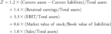
In his initial study, a Z-score of lower than 1.81 predicted failure and the model was able to accurately classify 95 percent of companies studied into a failure group and a nonfailure group. The original model was designed for manufacturing companies. Subsequent refinements to the models allow for other company types and time periods. Generally, the variables found to be useful in prediction include profitability ratios, coverage ratios, liquidity ratios, capitalization ratios, and earnings variability (Altman 2000).
Similar research has been performed on the ability of ratios to predict bond ratings and bond yields. For example, Ederington, Yawtiz, and Roberts (1987) found that a small number of variables (total assets, interest coverage, leverage, variability of coverage, and subordination status) were effective in explaining bond yields. Similarly, Ederington (1986) found that nine variables in combination could correctly classify more than 70 percent of bond ratings. These variables included ROA, long-term debt to assets, interest coverage, cash flow to debt, variability of coverage and cash flow, total assets, and subordination status. These studies have shown that ratios are effective in evaluating credit risk, bond yields, and bond ratings.
7. BUSINESS AND GEOGRAPHIC SEGMENTS
Analysts often need to evaluate the performance underlying business segments (subsidiary companies, operating units, or simply operations in different geographic areas) to understand in detail the company as a whole. Although companies are not required to provide full financial statements for segments, they are required to provide segment information under both IFRS and U.S. GAAP.23
7.1. Segment Reporting Requirements
An operating segment is defined as a component of a company: (a) that engages in activities that may generate revenue and create expenses, including a start-up segment that has yet to earn revenues, (b) whose results are regularly reviewed by the company’s senior management, and (c) for which discrete financial information is available.24 A company must disclose separate information about any operating segment which meets certain quantitative criteria—namely, the segment constitutes 10 percent or more of the combined operating segments’ revenue, assets, or profit. (For purposes of determining whether a segment constitutes 10 percent or more of combined profits or losses, the criteria is expressed in terms of the absolute value of the segment’s profit or loss as a percentage of the greater of (i) the combined profits of all profitable segments and (ii) the absolute amount of the combined losses of all loss-making segments.) If, after applying these quantitative criteria, the combined revenue from external customers for all reportable segments combined is less than 75 percent of the total company revenue, the company must identify additional reportable segments until the 75 percent level is reached. Small segments might be combined as one if they share a substantial number of factors that define a business or geographical segment, or they might be combined with a similar significant reportable segment. Information about operating segments and businesses that are not reportable is combined in an “all other segments” category.
Companies may internally report business results in a variety of ways (e.g., product segments and geographical segments). Companies identify the segments for external reporting purposes considering the definition of an operating segment and using factors such as what information is reported to the board of directors and whether a manager is responsible for each segment. Companies must disclose the factors used to identify reportable segments and the types and products and services sold by each reportable segment.
For each reportable segment, the following should also be disclosed:
- A measure of profit or loss.
- A measure of total assets and liabilities25 (if these amounts are regularly reviewed by the company’s chief decision-making officer).
- Segment revenue, distinguishing between revenue to external customers and revenue from other segments.
- Interest revenue and interest expense.
- Cost of property, plant, and equipment, and intangible assets acquired.
- Depreciation and amortization expense.
- Other noncash expenses.
- Income tax expense or income.
- Share of the net profit or loss of an investment accounted for under the equity method.
Companies also must provide a reconciliation between the information of reportable segments and the consolidated financial statements in terms of segment revenue, profit or loss, assets, and liabilities.
Another disclosure required is the company’s reliance on any single customer. If any single customer represents 10 percent or more of the company’s total revenues, the company must disclose that fact. From an analysts’ perspective, information about a concentrated customer base can be useful in assessing the risks faced by the company.
7.2. Segment Ratios
Based on the segment information that companies are required to present, a variety of useful ratios can be computed, as shown in Exhibit 7-21.
EXHIBIT 7-21 Definitions of Segment Ratios
| Segment Ratios | Numerator | Denominator |
| Segment margin | Segment profit (loss) | Segment revenue |
| Segment turnover | Segment revenue | Segment assets |
| Segment ROA | Segment profit (loss) | Segment assets |
| Segment debt ratio | Segment liabilities | Segment assets |
The segment margin measures the operating profitability of the segment relative to revenues, whereas the segment ROA measures the operating profitability relative to assets. Segment turnover measures the overall efficiency of the segment: how much revenue is generated per unit of assets. The segment debt ratio examines the level of liabilities (hence solvency) of the segment. Example 7-17 demonstrates the evaluation of segment ratios.
EXAMPLE 7-17 The Evaluation of Segment Ratios
The information contained in Exhibit 7-22 relates to the business segments of Groupe Danone (EuronextParis: BN) for 2008 and 2009 in millions of euro. According to the company’s 2009 annual report:
Over the course of the past 10 years, the Group has refocused its activities on the health food industry. On October 31, 2007, the acquisition of Royal Numico N.V. and its subsidiaries (“Numico”), a group specialized in baby nutrition and medical nutrition, marked a new phase in the Group’s development by adding these lines of business to Danone’s portfolio. The Group has since operated in four markets corresponding to its four business lines: (i) Fresh Dairy Products, (ii) Waters, (iii) Baby Nutrition, and (iv) Medical Nutrition.
Evaluate the performance of the segments using the segment margin, segment ROA, and segment turnover.
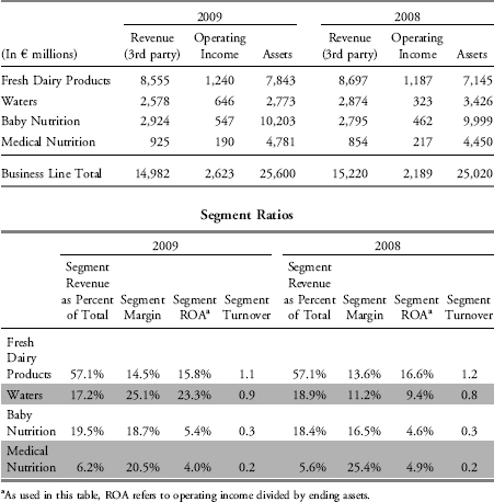
Solution: The waters segment (Evian and Volvic) was the most profitable in 2009 as measured by margin and ROA; however, in 2009 the segment did not grow as fast as the company’s other segments. In 2008, the segment represented 18.9 percent of total segment revenues, but in 2009 the percentage was only 17.2 percent.
The company’s largest segment by revenue, fresh dairy products, had the lowest margin in 2009 but a much higher segment ROA than the baby and medical nutrition segments. Medical nutrition is the second highest segment in terms of segment margin but lowest in turnover (an indicator of efficiency, i.e., the ability to generate revenue from assets). As a result, medical nutrition had the lowest segment ROA (Segment ROA=Segment operating income/Segment assets=(Segment operating income/Segment revenue) × (Segment revenue × Segment Assets)=Segment margin × Segment turnover. Reported percentages may differ due to rounding). Part of the explanation for segment differences in ROA may be that the medical and baby nutrition businesses were acquired in 2007. In an acquisition, the acquiring company reports the acquired assets at fair value at the time of the acquisition. Most of a company’s other assets are reported at historical costs, and over time, most long-term assets are depreciated. Thus, compared to assets in other segments, it is likely that the assets of the nutrition segments are reported at amounts more reflective of current prices.
8. MODEL BUILDING AND FORECASTING
Analysts often need to forecast future financial performance. For example, EPS forecasts of analysts are widely followed by Wall Street. Analysts use data about the economy, industry, and company in arriving at a company’s forecast. The results of an analyst’s financial analysis, including common-size and ratio analyses, are integral to this process, along with the judgment of the analysts.
Based upon forecasts of growth and expected relationships among the financial statement data, the analyst can build a model (sometimes referred to as an “earnings model”) to forecast future performance. In addition to budgets, pro forma financial statements are widely used in financial forecasting within companies, especially for use by senior executives and boards of directors. Last but not least, these budgets and forecasts are also used in presentations to credit analysts and others in obtaining external financing.
For example, based on a revenue forecast, an analyst may budget expenses based on expected common-size data. Forecasts of balance sheet and cash flow statements can be derived from expected ratio data, such as DSO. Forecasts are not limited to a single point estimate but should involve a range of possibilities. This can involve several techniques:
- Sensitivity analysis: Also known as “what if” analysis, sensitivity analysis shows the range of possible outcomes as specific assumptions are changed; this could, in turn, influence financing needs or investment in fixed assets.
- Scenario analysis: This type of analysis shows the changes in key financial quantities that result from given (economic) events, such as the loss of customers, the loss of a supply source, or a catastrophic event. If the list of events is mutually exclusive and exhaustive and the events can be assigned probabilities, the analyst can evaluate not only the range of outcomes but also standard statistical measures such as the mean and median value for various quantities of interest.
- Simulation: This is computer-generated sensitivity or scenario analysis based on probability models for the factors that drive outcomes. Each event or possible outcome is assigned a probability. Multiple scenarios are then run using the probability factors assigned to the possible values of a variable.
Financial analysis techniques, including common-size and ratio analysis, are useful in summarizing financial reporting data and evaluating the performance and financial position of a company. The results of financial analysis techniques provide important inputs into security valuation. Key facets of financial analysis include the following:
- Common-size financial statements and financial ratios remove the effect of size, allowing comparisons of a company with peer companies (cross-sectional analysis) and comparison of a company’s results over time (trend or time-series analysis).
- Activity ratios measure the efficiency of a company’s operations, such as collection of receivables or management of inventory. Major activity ratios include inventory turnover, days of inventory on hand, receivables turnover, days of sales outstanding, payables turnover, number of days of payables, working capital turnover, fixed asset turnover, and total asset turnover.
- Liquidity ratios measure the ability of a company to meet short-term obligations. Major liquidity ratios include the current ratio, quick ratio, cash ratio, and defensive interval ratio.
- Solvency ratios measure the ability of a company to meet long-term obligations. Major solvency ratios include debt ratios (including the debt-to-assets ratio, debt-to-capital ratio, debt-to-equity ratio, and financial leverage ratio) and coverage ratios (including interest coverage and fixed charge coverage).
- Profitability ratios measure the ability of a company to generate profits from revenue and assets. Major profitability ratios include return on sales ratios (including gross profit margin, operating profit margin, pretax margin, and net profit margin) and return on investment ratios (including operating ROA, ROA, return on total capital, ROE, and return on common equity).
- Ratios can also be combined and evaluated as a group to better understand how they fit together and how efficiency and leverage are tied to profitability.
- ROE can be analyzed as the product of the net profit margin, asset turnover, and financial leverage. This decomposition is sometimes referred to as DuPont analysis.
- Valuation ratios express the relation between the market value of a company or its equity (for example, price per share) and some fundamental financial metric (for example, earnings per share).
- Ratio analysis is useful in the selection and valuation of debt and equity securities and is a part of the credit rating process.
- Ratios can also be computed for business segments to evaluate how units within a business are performing.
- The results of financial analysis provide valuable inputs into forecasts of future earnings and cash flow.
1. Comparison of a company’s financial results to other peer companies for the same time period is called:
A. technical analysis.
B. time-series analysis.
C. cross-sectional analysis.
2. In order to assess a company’s ability to fulfill its long-term obligations, an analyst would most likely examine:
A. activity ratios.
B. liquidity ratios.
C. solvency ratios.
3. Which ratio would a company most likely use to measure its ability to meet short-term obligations?
A. Current ratio
B. Payables turnover
C. Gross profit margin
4. Which of the following ratios would be most useful in determining a company’s ability to cover its lease and interest payments?
A. ROA
B. Total asset turnover
C. Fixed charge coverage
5. An analyst is interested in assessing both the efficiency and liquidity of Spherion PLC. The analyst has collected the following data for Spherion:
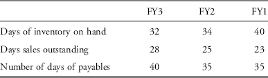
Based on this data, what is the analyst least likely to conclude?
A. Inventory management has contributed to improved liquidity.
B. Management of payables has contributed to improved liquidity.
C. Management of receivables has contributed to improved liquidity.
6. An analyst is evaluating the solvency and liquidity of Apex Manufacturing and has collected the following data (in millions of euro):
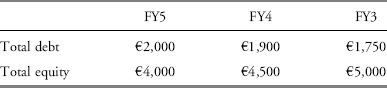
Which of the following would be the analyst’s most likely conclusion?
A. The company is becoming increasingly less solvent, as evidenced by the increase in its debt-to-equity ratio from 0.35 to 0.50 from FY3 to FY5.
B. The company is becoming less liquid, as evidenced by the increase in its debt-to-equity ratio from 0.35 to 0.50 from FY3 to FY5.
C. The company is becoming increasingly more liquid, as evidenced by the increase in its debt-to-equity ratio from 0.35 to 0.50 from FY3 to FY5.
7. With regard to the data in Problem 6, what would be the most reasonable explanation of the financial data?
A. The decline in the company’s equity results from a decline in the market value of this company’s common shares.
B. The €250 increase in the company’s debt from FY3 to FY5 indicates that lenders are viewing the company as increasingly creditworthy.
C. The decline in the company’s equity indicates that the company may be incurring losses, paying dividends greater than income, and/or repurchasing shares.
8. An analyst observes a decrease in a company’s inventory turnover. Which of the following would most likely explain this trend?
A. The company installed a new inventory management system, allowing more efficient inventory management.
B. Due to problems with obsolescent inventory last year, the company wrote off a large amount of its inventory at the beginning of the period.
C. The company installed a new inventory management system but experienced some operational difficulties resulting in duplicate orders being placed with suppliers.
9. Which of the following would best explain an increase in receivables turnover?
A. The company adopted new credit policies last year and began offering credit to customers with weak credit histories.
B. Due to problems with an error in its old credit scoring system, the company had accumulated a substantial amount of uncollectible accounts and wrote off a large amount of its receivables.
C. To match the terms offered by its closest competitor, the company adopted new payment terms now requiring net payment within 30 days rather than 15 days, which had been its previous requirement.
10. Brown Corporation had average days of sales outstanding of 19 days in the most recent fiscal year. Brown wants to improve its credit policies and collection practices and decrease its collection period in the next fiscal year to match the industry average of 15 days. Credit sales in the most recent fiscal year were $300 million, and Brown expects credit sales to increase to $390 million in the next fiscal year. To achieve Brown’s goal of decreasing the collection period, the change in the average accounts receivable balance that must occur is closest to:
A. +$0.41 million.
B. −$0.41 million.
C. −$1.22 million.
11. An analyst observes the following data for two companies:
| Company A | Company B | |
| Revenue | $4,500 | $6,000 |
| Net income | $50 | $1,000 |
| Current assets | $40,000 | $60,000 |
| Total assets | $100,000 | $700,000 |
| Current liabilities | $10,000 | $50,000 |
| Total debt | $60,000 | $150,000 |
| Shareholders’ equity | $30,000 | $500,000 |
Which of the following choices best describes reasonable conclusions that the analyst might make about the two companies’ ability to pay their current and long-term obligations?
A. Company A’s current ratio of 4.0 indicates it is more liquid than Company B, whose current ratio is only 1.2, but Company B is more solvent, as indicated by its lower debt-to-equity ratio.
B. Company A’s current ratio of 0.25 indicates it is less liquid than Company B, whose current ratio is 0.83, and Company A is also less solvent, as indicated by a debt-to-equity ratio of 200 percent compared with Company B’s debt-to-equity ratio of only 30 percent.
C. Company A’s current ratio of 4.0 indicates it is more liquid than Company B, whose current ratio is only 1.2, and Company A is also more solvent, as indicated by a debt-to-equity ratio of 200 percent compared with Company B’s debt-to-equity ratio of only 30 percent.