
CHAPTER 8
FINANCIAL STATEMENT ANALYSIS: APPLICATIONS
After completing this chapter, you will be able to do the following:
- Evaluate a company’s past financial performance and explain how a company’s strategy is reflected in past financial performance.
- Prepare a basic projection of a company’s future net income and cash flow.
- Describe the role of financial statement analysis in assessing the credit quality of a potential debt investment.
- Describe the use of financial statement analysis in screening for potential equity investments.
- Determine and justify appropriate analyst adjustments to a company’s financial statements to facilitate comparison with another company.
This reading presents several important applications of financial statement analysis. Among the issues we will address are the following:
- What are the key questions to address in evaluating a company’s past financial performance?
- How can an analyst approach forecasting a company’s future net income and cash flow?
- How can financial statement analysis be used to evaluate the credit quality of a potential fixed-income investment?
- How can financial statement analysis be used to screen for potential equity investments?
- How can differences in accounting methods affect financial ratio comparisons between companies, and what are some adjustments analysts make to reported financials to facilitate comparability among companies.
Chapter 1, “Financial Statement Analysis: An Introduction,” described a framework for conducting financial statement analysis. Consistent with that framework, prior to undertaking any analysis, an analyst should explore the purpose and context of the analysis. The purpose and context guide further decisions about the approach, the tools, the data sources, and the format in which to report results of the analysis, and also suggest which aspects of the analysis are most important. Having identified the purpose and context, the analyst should then be able to formulate the key questions that the analysis must address. The questions will suggest the data the analyst needs to collect to objectively address the questions. The analyst then processes and analyzes the data to answer these questions. Conclusions and decisions based on the analysis are communicated in a format appropriate to the context, and follow-up is undertaken as required. Although this reading will not formally present applications as a series of steps, the process just described is generally applicable.
Section 2 of this reading describes the use of financial statement analysis to evaluate a company’s past financial performance, and Section 3 describes basic approaches to projecting a company’s future financial performance. Section 4 presents the use of financial statement analysis in assessing the credit quality of a potential debt investment. Section 5 concludes the survey of applications by describing the use of financial statement analysis in screening for potential equity investments. Analysts often encounter situations in which they must make adjustments to a company’s reported financial results to increase their accuracy or comparability with the financials of other companies. Section 6 illustrates several common types of analyst adjustments. Section 7 presents a summary, and practice problems in the CFA Institute multiple-choice format conclude the reading.
2. APPLICATION: EVALUATING PAST FINANCIAL PERFORMANCE
Analysts examine a company’s past financial performance for a number of reasons. Cross-sectional analysis of financial performance facilitates understanding of the comparability of companies for a market-based valuation.1 Analysis of a company’s historical performance over time can provide a basis for a forward-looking analysis of the company. Both cross-sectional and trend analysis can provide information for evaluating the quality and performance of a company’s management.
An evaluation of a company’s past performance addresses not only what happened (i.e., how the company performed) but also why it happened—the causes behind the performance and how the performance reflects the company’s strategy. Evaluative judgments assess whether the performance is better or worse than a relevant benchmark, such as the company’s own historical performance, a competitor’s performance, or market expectations. Some key analytical questions include the following:
- How and why have corporate measures of profitability, efficiency, liquidity, and solvency changed over the periods being analyzed?
- How do the level and trend in a company’s profitability, efficiency, liquidity, and solvency compare with the corresponding results of other companies in the same industry? What factors explain any differences?
- What aspects of performance are critical for a company to successfully compete in its industry, and how did the company perform relative to those critical performance aspects?
- What are the company’s business model and strategy, and how did they influence the company’s performance as reflected in, for example, its sales growth, efficiency, and profitability?
Data available to answer these questions include the company’s (and its competitors’) financial statements, materials from the company’s investor relations department, corporate press releases, and nonfinancial-statement regulatory filings, such as proxies. Useful data also include industry information (e.g., from industry surveys, trade publications, and government sources), consumer information (e.g., from consumer satisfaction surveys), and information that is gathered by the analyst firsthand (e.g., through on-site visits). Processing the data typically involves creating common-size financial statements, calculating financial ratios, and reviewing or calculating industry-specific metrics. Example 8-1 illustrates the effects of strategy on performance and the use of basic economic reasoning in interpreting results.
EXAMPLE 8-1 A Change in Strategy Reflected in Financial Performance
Apple Inc. (NASDAQ: AAPL) is a company that has evolved and adapted over time. In its 1994 Prospectus (Form 424B5) filed with the U.S. SEC, Apple identified itself as “one of the world’s leading personal computer technology companies.” At that time, most of its revenue was generated by computer sales. In the prospectus, however, Apple stated, “The Company’s strategy is to expand its market share in the personal computing industry while developing and expanding into new related business such as Personal Interactive Electronics and Apple Business Systems.” Over time, products other than computers became significant generators of revenue and profit. In its 2010 Annual Report (Form 10-K) filed with the SEC, Apple stated in Part I, Item 1, under Business Strategy, “The Company is committed to bringing the best user experience to its customers through its innovative hardware, software, peripherals, services, and Internet offerings. The Company’s business strategy leverages its unique ability to design and develop. . .to provide its customers new products and solutions with superior ease-of-use, seamless integration, and innovative industrial design.. . .The Company is therefore uniquely positioned to offer superior and well-integrated digital lifestyle and productivity solutions.” Clearly, the company is no longer simply a personal computer technology company.
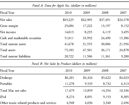
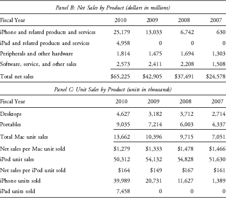
In analyzing the historical performance of Apple as of the beginning of 2011, an analyst might refer to the information presented in Exhibit 8-1. Panel A presents selected financial data for the company from 2007 to 2010. Panels B and C present excerpts from the segment footnote. Panel B reports the net sales by product, in millions of dollars, and Panel C reports the unit sales by product, in thousands. [Because Apple manages its business on the basis of geographical segments, the more complete data required in segment reporting (i.e., segment operating income and segment assets) is available only by geographical segment, not by product.]
In 2005, an article in Barron’s said, “In the last year, the iPod has become Apple’s best-selling product, bringing in a third of revenues for the Cupertino, Calif. firm. . .Little noticed by these iPod zealots, however is a looming threat. . .Wireless phone companies are teaming up with the music industry to make most mobile phones into music players” (Barron’s 27 June 2005, p. 19). The threat noted by Barron’s was not unnoticed or ignored by Apple.
In June 2007, Apple itself entered the mobile phone market with the launch of the original iPhone, followed in June 2008 by the second-generation iPhone 3G (a handheld device combining the features of a mobile phone, an iPod, and an Internet connection device). Soon after, the company launched the iTunes App Store, which allows users to download third-party applications onto their iPhones. As noted in a 2009 BusinessWeek article, Apple “is the world’s largest music distributor, having passed Wal-Mart Stores in early 2008. Apple sells around 90% of song downloads and 75% of digital music players in the U.S.” (BusinessWeek, 28 September 2009, p. 34). Product innovations continue as evidenced by the introduction of the iPad in January 2010.
EXHIBIT 8-1 Selected Data for Apple Inc. (for the Four Years Ended 25 September 2010)
Source: Apple Inc. 2008 Form 10-K, 2009 Form 10-K/A, and 2010 Form 10-K.
Using the information provided, address the following:
1. Typically, products that are differentiated either through recognizable brand names, proprietary technology, unique styling, or some combination of these features can be sold at a higher price than commodity products.
A. In general, would the selling prices of differentiated products be more directly reflected in a company’s operating profit margin or gross profit margin?
B. Does Apple’s financial data (Panel A) reflect a successful differentiation strategy?
2. How liquid is Apple at the end of fiscal 2009 and 2010? In general, what are some of the considerations that a company makes in managing its liquidity?
3. Based on the product segment data for 2007 (Panels B and C), Apple’s primary source of revenue was from sales of computers (the $10,336 million in sales of Mac computers represented 42 percent of total net sales) and its secondary source of revenue was from iPods. How has the company’s product mix changed since 2007, and what might this change suggest for an analyst examining Apple relative to its competitors?
Solution to 1:
A. Sales of differentiated products at premium prices would generally be reflected more directly in the gross profit margin; such sales would have a higher gross profit margin, all else equal. The effect of premium pricing generally would also be reflected in a higher operating margin. Expenditures on advertising and/or research are required to support differentiation, however, which means that the effect of premium pricing on operating profit margins is often weaker than the effect on gross profit margins.
B. Based on Apple’s financial data in Panel A, the company appears to have successfully implemented a differentiation strategy, with gross margin increasing from 33 percent of sales to 40 percent of sales, as shown in the following table:
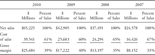
In general, in addition to a successful differentiation strategy, higher gross margins can result from lower input costs and/or a change in sales mix to include more product types with high gross margins.
Solution to 2: Apple was very liquid at the end of fiscal 2009 and 2010, with current ratios of, respectively, 2.7 (=$31,555/$11,506) and 2.0 (=$41,678/$20,722). In addition, the company had 71.6 and 67.8 percent of total assets invested in cash and marketable securities at the end of, respectively, 2009 and 2010. In general, some of the considerations that a company makes in managing its liquidity include the following: (1) maintaining enough cash and other liquid assets to ensure that it can meet near-term operating expenditures and unexpected needs, (2) avoiding excessive amounts of cash because the return on cash assets is almost always less than the company’s costs of capital to finance its assets, and (3) accumulating cash that will be used for acquisitions (sometimes referred to as a “war chest,” which is illustrated in Exhibit 8-2). Apple may be accumulating a war chest, but an analyst might, given point 2, question the amount of cash and marketable securities on hand.
Solution to 3: In 2009, the proportion of Apple’s total sales from computers declined from 42 percent to 32 percent and the proportion of total sales from iPods declined from 34 percent to 19 percent. The biggest shift in product sales was the increase in iPhone sales from 3 percent in 2007, the year of the product’s introduction, to 30 percent in 2009. In 2010, the proportion of Apple’s total sales from computers and iPods continued to decline and the proportion from iPhones continued to increase. These proportions in 2010 were, respectively, 27 percent, 13 percent, and 39 percent of total sales. The iPad introduced in fiscal 2010 represented 8 percent of total sales that year. For an analyst examining Apple relative to its competitors, the relevant comparable companies clearly changed from 2007 to 2010. Recently, the company may be more appropriately compared not only with other computer manufacturers but also with mobile phone manufacturers and companies developing competing software and systems for mobile Internet devices. Apple’s product innovation has reshaped the competitive landscape.
To illustrate the use of a war chest, Exhibit 8-2 provides descriptions of several companies’ cash positions and potential uses of their funds. When a company has accumulated large amounts of cash, an analyst should consider the likely implications for a company’s strategic actions (i.e., potential acquisitions) or financing decisions (e.g., share buybacks, dividends, or debt repayment).
EXHIBIT 8-2 War Chests
The expression “war chest” is sometimes used to refer to large cash balances that a company accumulates prior to making acquisitions. Some examples are shown here:
Apple Inc.
Apple (NASDAQ: AAPL) closed 2009 with nearly $40 billion in the bank, in the form of cash, short-term and long-term marketable securities. That “war chest,” as one shareholder described it [during Apple’s annual shareholder’s meeting], has fueled speculation about what the company might do with the funds. Options could include large acquisitions or returning cash to shareholders in the form of a buyback or dividend.
Dan Gallagher, MarketWatch, 25 February 2010
Asahi Breweries
The head of Japan’s Asahi Breweries said he expects to have $9.2 billion on tap for acquisitions over the next five years as it looks for new growth drivers outside the shrinking domestic beer market. Asahi President Naoki Izumiya also told Reuters that he wanted to lift its stake in China’s Tsingtao Brewery pending regulatory changes, and is eyeing closer ties in South Korea with that country’s top soft drinks maker, the Lotte Group.
Taiga Uranaka and Ritsuko Shimizu, Reuters, Tuesday, 3 August 2010
McLeod Russel India Ltd.
McLeod Russel India Ltd., the world’s biggest tea grower, plans to use rising prices to build a “war chest” of as much as $250 million to acquire companies.. . .The plantation company, based in Kolkata, may buy tea companies in India and Africa as it targets a 50 percent increase in production to 150 million kilograms in three to four years, said Aditya Khaitan, managing director of McLeod Russel.
Arijit Ghosh and Thomas Kutty Abraham, Bloomberg, 14 May 2010
In calculating and interpreting financial statement ratios, an analyst needs to be aware of the potential impact on the financial statements and related ratios of companies reporting under different accounting standards, such as international financial reporting standards (IFRS), U.S. generally accepted accounting principles (U.S. GAAP), or other home-country GAAP. Furthermore, even within a given set of accounting standards, companies still have discretion to choose among acceptable methods. A company also may make different assumptions and estimates even when applying the same method as another company. Therefore, making selected adjustments to a company’s financial statement data may be useful to facilitate comparisons with other companies or with the industry overall. Examples of such analyst adjustments will be discussed in Section 6.
Non-U.S. companies that use any acceptable body of accounting standards (other than IFRS or U.S. GAAP) and file with the U.S. SEC (because their shares or depositary receipts based on their shares trade in the United States) are required to reconcile their net income and shareholders’ equity accounts to U.S. GAAP. Note that in 2007, the SEC eliminated the reconciliation requirement for non-U.S. companies using IFRS and filing with the SEC. Example 8-2 uses reconciliation data from SEC filings to illustrate how differences in accounting standards can affect financial ratio comparisons. The differences in the example are very large.
EXAMPLE 8-2 The Effect of Differences in Accounting Standards on ROE Comparisons
In the process of comparing the 2009 performance of three telecommunication companies—Teléfonos de México, S.A.B. DE C.V. (NYSE: TMX), Tele Norte Leste Participações S.A. (NYSE: TNE), and Verizon Communications Inc. (NYSE: VZ)—an analyst prepared Exhibit 8-3 to evaluate whether the differences in accounting standards affect the comparison of the three companies’ return on equity (ROE). Panel A presents selected data for TMX for 2008 and 2009 under Mexican GAAP and U.S. GAAP. Panel B presents data for TNE under Brazilian GAAP and U.S. GAAP. Panel C presents data for VZ under U.S. GAAP.
EXHIBIT 8-3 Data for TMX, TNE, and VZ for a ROE Calculation (Years Ended 31 December)
Sources: TMX’s and TME’s 2009 Form 20-F; VZ’s 2009 10-K.
| Panel A: Selected Data for Teléfonos de México (TMX) | ||
| (in millions of Mexican pesos) | 2009 | 2008 |
| Mexican GAAP | ||
| Net income | 20,469 | 20,177 |
| Shareholders’ equity | 38,321 | 39,371 |
| U.S. GAAP | ||
| Net income | 19,818 | 19,782 |
| Shareholders’ equity | 7,465 | 11,309 |
| Panel B: Selected Data for Tele Norte Leste Participações S.A. (TNE) | ||
| (in millions of Brazilian reais) | 2009 | 2008 |
| Brazilian GAAP | ||
| Net income | (1,056) | 1,432 |
| Shareholders’ equity | 15,352 | 11,411 |
| U.S. GAAP | ||
| Net income | 4,866 | 1,252 |
| Shareholders’ equity | 21,967 | 11,203 |
| Panel C: Selected Data for Verizon Communications Inc. | ||
| (in millions of U.S. dollars) | 2009 | 2008 |
| U.S. GAAP | ||
| Net income | 10,358 | 12,583 |
| Shareholders’ equity | 84,367 | 78,905 |
a“Reais” is the plural of “real.”
Based on TMX’s reconciliation footnote, the most significant adjustment for TMX between Mexican GAAP and U.S. GAAP was an adjustment to shareholders’ equity for “Labor obligations (SFAS 158).” The U.S. accounting standard SFAS 158, Employers’ Accounting for Defined Benefit Pension and Other Postretirement Plans, now codified as Accounting Standards Codification (ASC) 715 (i.e., Expenses: Compensation–Retirement Benefits) requires companies to reflect on their balance sheets the funded status of pensions and other post-employment benefits. (Funded status equals plan assets minus plan obligations.) For an underfunded plan—i.e., one in which assets that are held in trust to pay for the obligation are less than the amount of the obligation—the amount of underfunding is shown as a liability and as a reduction to shareholders’ equity. [The full reconciliation between shareholders’ equity under Mexican FRS and U.S. GAAP (not presented here) shows that the adjustment related to SFAS 158 reduced equity at TMX by 50,028 million pesos and 46,637 million pesos in 2009 and 2008, respectively.]
Based on TNE’s reconciliation footnote, the most significant adjustment for TNE between Brazilian GAAP and U.S. GAAP was an increase to net income to recognize a “bargain purchase gain on business combination.” A bargain purchase gain under U.S. GAAP results when the purchase price of an acquisition is less than the fair value (as of the acquisition date) of the net identified assets acquired. The adjustment for the bargain purchase gain represented an increase of 6,591 million Brazilian reais to net income as reported under Brazilian GAAP.
Does the difference in accounting standards affect the ROE comparison?
Solution: When ROE is compared under different standards, both of the non-U.S. companies report significantly higher ROE under U.S. GAAP than under home-country GAAP (Mexican GAAP for TMX and Brazilian GAAP for TNE).
When ROE is compared across companies, TMX’s ROE is higher than that of both of the other two companies regardless of whether the comparison is based on home-country amounts or U.S. GAAP amounts. For TNE, however, the company reported a loss and thus a negative ROE under home-country (Brazilian) GAAP but a profit under U.S. GAAP. The ROE for TNE is lower than VZ’s ROE when calculations are based on home-country GAAP but higher than VZ’s ROE when calculations are based on U.S. GAAP.
Results of the calculations are summarized in the following table, with the calculations based on TMX’s Mexican GAAP explained after the table:
| Panel A: Teléfonos de México (TMX) | |
| Mexican GAAP | |
| Return on average shareholders’ equity | 52.69% |
| U.S. GAAP | |
| Return on average shareholders’ equity | 211.12% |
| Panel B: Tele Norte Leste Participações S.A. (TNE) | |
| Brazilian GAAP | |
| Return on average shareholders’ equity | −7.89% |
| U.S. GAAP | |
| Return on average shareholders’ equity | 29.34% |
| Panel C: Verizon Communications Inc. (VZ) | |
| U.S. GAAP | |
| Return on average shareholders’ equity | 12.69% |
For an illustration of the ROE calculation, we have calculated TMX’s ROE (with all numbers in thousands of Mexican pesos) as 20,468,983/[(38,320,773+39,371,099)/2]=52.69%. Note that TMX’s significantly higher ROE under U.S. GAAP is the result of a much lower shareholders’ equity under U.S. GAAP than under Mexican GAAP.
In Example 8-2, the 2009 ROE for both TMX and TNE differed substantially under home-country GAAP and U.S. GAAP. In general, because the reconciliation data are no longer required by the SEC, we cannot determine whether differences in net income, equity, and thus ROE also exist between IFRS and the companies’ home-country GAAP (including U.S. GAAP). Historically, research indicates that for most non-U.S. companies filing with the SEC, differences in net income between U.S. GAAP and home-country GAAP average 1–2 percent of market value of equity, but large variations do occur.2 Additionally, research indicates that for most non-U.S. companies filing with the SEC, ROE was historically higher under IFRS than under U.S. GAAP.3
Comparison of the levels and trends in a company’s performance provide information about how the company performed. The company’s management presents its view about causes underlying its performance in the management commentary or management discussion and analysis (MD&A) section of its annual report and during periodic conference calls with analysts and investors. To gain additional understanding of the causes underlying a company’s performance, an analyst can review industry information or seek information from additional sources, such as consumer surveys.
The results of an analysis of past performance provide a basis for reaching conclusions and making recommendations. For example, an analysis undertaken as the basis for a forward-looking study might conclude that a company’s future performance is or is not likely to reflect continuation of recent historical trends. As another example, an analysis to support a market-based valuation of a company might focus on whether the company’s profitability and growth outlook, which is better (worse) than the peer group median, justifies its relatively high (low) valuation. This analysis would consider market multiples, such as price-to-earnings ratio (P/E), price-to-book ratio, and total invested capital to EBITDA (earnings before interest, taxes, depreciation, and amortization).4 As another example, an analysis undertaken as part of an evaluation of the management of two companies might result in conclusions about whether one company has grown as fast as another company, or as fast as the industry overall, and whether each company has maintained profitability while growing.
3. APPLICATION: PROJECTING FUTURE FINANCIAL PERFORMANCE
Projections of future financial performance are used in determining the value of a company or its equity component. Projections of future financial performance are also used in credit analysis—particularly in project finance or acquisition finance—to determine whether a company’s cash flows will be adequate to pay the interest and principal on its debt and to evaluate whether a company will likely remain in compliance with its financial covenants.
Sources of data for analysts’ projections include some or all of the following: the company’s projections, the company’s previous financial statements, industry structure and outlook, and macroeconomic forecasts.
Evaluating a company’s past performance may provide a basis for forward-looking analyses. An evaluation of a company’s business and economic environment and its history may persuade the analyst that historical information constitutes a valid basis for such analyses and that the analyst’s projections may be based on the continuance of past trends, perhaps with some adjustments. Alternatively, in the case of a major acquisition or divestiture, for a start-up company, or for a company operating in a volatile industry, past performance may be less relevant to future performance.
Projections of a company’s near-term performance may be used as an input to market-based valuation or relative valuation (i.e., valuation based on price multiples). Such projections may involve projecting next year’s sales and using the common-size income statement to project major expense items or particular margins on sales (e.g., gross profit margin or operating profit margin). These calculations will then lead to the development of an income measure for a valuation calculation, such as net income, earnings per share (EPS) or EBITDA. More complex projections of a company’s future performance involve developing a more detailed analysis of the components of performance for multiple periods—for example, projections of sales and gross margin by product line, projection of operating expenses based on historical patterns, and projection of interest expense based on requisite debt funding, interest rates, and applicable taxes. Furthermore, a projection should include sensitivity analyses applied to the major assumptions.
3.1. Projecting Performance: An Input to Market-Based Valuation
One application of financial statement analysis involves projecting a company’s near-term performance as an input to market-based valuation. For example, an analyst might project a company’s sales and profit margin to estimate EPS and then apply a projected P/E to establish a target price for the company’s stock.
Analysts often take a top-down approach to projecting a company’s sales.5 First, industry sales are projected on the basis of their historical relationship with some macroeconomic indicator, such as growth in real gross domestic product (GDP). In researching the automobile industry, for example, the analyst may find that the industry’s annual domestic unit car sales (number of cars sold in domestic markets) bears a relationship to annual changes in real GDP. Regression analysis is often used to establish the parameters of such relationships. Other factors in projecting sales may include consumer income or tastes, technological developments, and the availability of substitute products or services. After industry sales are projected, a company’s market share is projected. Company-level market share projections may be based on historical market share and a forward-looking assessment of the company’s competitive position. The company’s sales are then estimated as its projected market share multiplied by projected total industry sales.
After developing a sales forecast for a company, an analyst can choose among various methods for forecasting income and cash flow. An analyst must decide on the level of detail to consider in developing forecasts. For example, separate forecasts may be made for individual expense items or for more aggregated expense items, such as total operating expenses. Rather than stating a forecast in terms of expenses, the forecast might be stated in terms of a forecasted profit margin (gross, operating, or net). The net profit margin, in contrast to the gross or operating profit margins, is affected by financial leverage and tax rates, which are subject to managerial and legal/regulatory revisions; therefore, historical data may sometimes be more relevant for projecting gross or operating profit margins than for projecting net profit margins. Whatever the margin used, the forecasted amount of profit for a given period is the product of the forecasted amount of sales and the forecast of the selected profit margin.
As Example 8-3 illustrates, for relatively mature companies operating in nonvolatile product markets, historical information on operating profit margins can provide a useful starting point for forecasting future operating profits (at least over short forecasting horizons). Historical operating profit margins are typically less reliable for projecting future margins for a new or relatively volatile business or one with significant fixed costs (which can magnify the volatility of operating margins).
EXAMPLE 8-3 Using Historical Operating Profit Margins to Forecast Operating Profit
One approach to projecting operating profit is to determine a company’s average operating profit margin over the previous several years and apply that margin to a forecast of the company’s sales. Use the following information on three companies to answer Questions 1 and 2 following:
- Johnson & Johnson (JNJ). This U.S. health care conglomerate, founded in 1887, had 2009 sales of around $61.9 billion from its three main businesses: pharmaceuticals, medical devices and diagnostics, and consumer products.
- BHP Billiton (BHP). This company, with group headquarters in Australia and secondary headquarters in London, is the world’s largest natural resources company, reporting revenue of approximately US$50.2 billion for the fiscal year ended June 2009. The company mines, processes, and markets coal, copper, nickel, iron, bauxite, and silver and also has substantial petroleum operations.
- Baidu. This Chinese company, which was established in 2000 and went public on NASDAQ in 2005, is the leading Chinese language search engine. The company’s revenues for 2009 were 4.4 billion renminbi (RMB), an increase of 40 percent from 2008 and more than 14 times greater than revenues in 2005.
1. For each of the three companies, state and justify whether the suggested forecasting method (applying the average operating profit over the previous several years to a forecast of sales) would be a reasonable starting point for projecting future operating profit.
2. Assume that the 2009 forecast of sales was perfect and, therefore, equal to the realized sales by the company in 2009. Compare the forecast of 2009 operating profit, using an average of the previous four years’ operating profit margins, with the actual 2009 operating profit reported by the company given the following additional information:
- JNJ: For the four years prior to 2009, JNJ’s average operating profit margin was approximately 25.0 percent. The company’s actual operating profit for 2009 was $15.6 billion.
- BHP: For the four years prior to the year ending June 2009, BHP’s average operating profit margin was approximately 38.5 percent. The company’s actual operating profit for the year ended June 2009 was US$12.2 billion.
- Baidu: Over the four years prior to 2009, Baidu’s average operating profit margin was approximately 27.1 percent. The company’s actual operating profit for 2009 was RMB1.6 billion.
Using the additional information given, state and justify whether actual results support the usefulness of the stable operating margin assumption.
Solution to 1:
JNJ. Because JNJ is an established company with diversified operations in relatively stable businesses, the suggested approach to projecting the company’s operating profit would be a reasonable starting point.
BHP. Because commodity prices tend to be volatile and the mining industry is relatively capital intensive, the suggested approach to projecting BHP’s operating profit would probably not be a useful starting point.
Baidu. A relatively new company such as Baidu has limited operating history on which to judge stability of margins. The company appears to have been in a period of rapid growth and is in an industry that has been changing rapidly in recent years. This important aspect about the company suggests that the broad approach to projecting operating profit would not be a useful starting point for Baidu.
Solution to 2:
JNJ. JNJ’s actual operating profit margin for 2009 was 25.2 percent ($15.6 billion divided by sales of $61.9 billion), which is very close to the company’s three-year average operating profit margin of approximately 25.0 percent. If the average operating profit margin had been applied to perfectly forecasted 2009 sales to obtain forecasted operating profit, the forecasting error would have been minimal.
BHP. BHP’s actual operating profit margin for the year ended June 2009 was 24.3 percent ($12.2 billion divided by sales of $50.2 billion). If the company’s average profit margin of 38.5 percent had been applied to perfectly forecasted sales, the forecasted operating profit would have been approximately US$19.3 billion, around 58 percent higher than actual operating profit.
Baidu. Baidu’s actual operating profit margin for 2009 was 36.4 percent (RMB1.6 billion divided by sales of RMB4.4 billion). If the average profit margin of 27.1 percent had been applied to perfectly forecasted sales, the forecasted operating profit would have been approximately RMB1.2 billion, or around 25 percent below Baidu’s actual operating profit.
Although prior years’ profit margins can provide a useful starting point in projections for companies with relatively stable business, the underlying data should, nonetheless, be examined to identify items that are not likely to occur again in the following year(s). Such nonrecurring (i.e., transitory) items should be removed from computations of any profit amount or profit margin that will be used in projections. Example 8-4 illustrates this principle.
EXAMPLE 8-4 Issues in Forecasting
Following are excerpts from the annual reports of two global companies. Indicate the relevance of each disclosure in forecasting the company’s future net income. (Business descriptions are from the companies’ websites.)
1. Anheuser-Busch InBev SA/NV (Euronext: ABI, NYSE: BUD), the world’s largest brewing company by volume, with brands such as Budweiser, Stella Artois, and Beck’s, disclosed the following items, which are primarily related to its acquisition of Anheuser-Busch.
1.1 “The 2009 restructuring charges of (153)m US dollar primarily relate to the Anheuser-Busch integration, organizational alignments and outsourcing activities in the global headquarters, Western Europe and Asia Pacific. These changes aim to eliminate overlap or duplicated processes and activities across functions and zones. These one time expenses as a result of the series of decisions will provide the company with a lower cost base besides a stronger focus on AB InBev’s core activities, quicker decision-making and improvements to efficiency, service and quality.. . .
1.2 “2009 business and asset disposals resulted in an exceptional income of 1,541m US dollar mainly representing the sale of assets of InBev USA LLC (also doing business under the name Labatt USA) to an affiliate of KPS Capital Partners, L.P. (54m US dollar), the sale of the Korean subsidiary Oriental Brewery to an affiliate of Kohlberg Kravis Roberts & Co. L.P. (428m US dollar) and the sale of the Central European operations to CVC Capital Partners (1,088m US dollar).. . .”
Source: 2009 Annual Report, note 8.
2. Nestlé Group (NESN.VX), the largest food and beverages manufacturer in the world, disclosed the following information about the sale of its holding in the eye care company Alcon Inc. (NYSE: ACL).
2.1 “The most significant divestment was announced on 4 January 2010, with the agreement to sell our remaining holding in Alcon, for about USD 28 billion. The completion of this transaction will bring the total value realized from the three-part disposal of Alcon to over USD 40 billion. Alcon was acquired by Nestlé in 1977 for USD 280 million.”
Source: 2009 Annual Report, Shareholder Letter, p. 4.
2.2 “On 7 July 2008, the Group sold 24.8% of Alcon outstanding capital to Novartis for a total amount of USD 10.4 billion, resulting in a profit on disposal of CHF 9208 million and in an increase of noncontrolling interests of CHF 1537 million. The agreement further included the option for Novartis to acquire Nestlé’s remaining shareholding in Alcon at a price of USD 181.– per share from January 2010 until July 2011. During the same period, Nestlé had the option to sell its remaining shareholding in Alcon to Novartis at the lower of either the call price of USD 181.– per share or the average share price during the week preceding the exercise plus a premium of 20.5%. On 4 January 2010, Novartis exercised its call option to acquire the remaining 52% shareholding from Nestlé at a price of USD 181.– per share. The transaction is now pending regulatory approval which can be expected during the course of 2010. As IFRS 5 criteria were met on 31 December 2009, Alcon’s related assets and liabilities are classified as a disposal group in Assets held for sale and Liabilities directly associated with assets held for sale. Moreover, Alcon operations are disclosed as discontinued operations in the 2009 Consolidated Financial Statements. The results of Alcon discontinued operations are disclosed separately in the income statement.”
Source: 2009 Financial Statements, note 25
2.3 Excerpt from Nestlé’s Consolidated Income Statement for the Year Ended 31 December 2009:
Source: 2009 Financial Statements.
| (CHF millions) | ||
| 2009 | 2008 | |
| Sales | ||
| Continuing operations | 100,579 | 103,086 |
| Discontinued operations | 7,039 | 6,822 |
| Total | 107,618 | 109,908 |
| EBIT (earnings before interest, taxes, restructuring, and impairments) | ||
| Continuing operations | 13,222 | 13,240 |
| Discontinued operations | 2,477 | 2,436 |
| Total | 15,699 | 15,676 |
| Profit for the year | ||
| Continuing operations | 9,551 | 7,656 |
| Discontinued operations | 2,242 | 11,395 |
| Total | 11,793 | 19,051 |
Discussion of 1.1: This item relates to one-time restructuring charges aimed at eliminating duplication between the pre-acquisition operations of the two companies (InBev and Anheuser-Busch). The restructuring charges themselves are not directly relevant in forecasting the future net income of the company. If the restructuring successfully reduced the company’s cost base, however, the combined companies’ expenses in the future are likely to be less than the sum of the two individual companies’ expenses. Also, if the cost base was successfully reduced, the profit margin for the combined company is likely to be higher than a profit margin calculated as the sum of the individual companies’ profits divided by the sum of the individual companies’ sales revenues.
Discussion of 1.2: Gains on sales of businesses and assets that result in exceptional income are not a core part of a company’s business. This item should typically not be viewed as an ongoing source of earnings and should not, therefore, be a component of forecasts of net income. Additionally, any portion of the company’s past income that had been generated by the businesses sold should be excluded from forecasted net income.
Discussion of 2.1: These disclosures pertain to Nestlé’s total USD40 billion return on the USD280 million investment in Alcon over 33 years (between 1977 and 2010). The information is not directly relevant to forecasting future net income. Although forecasts of net income must exclude the income from the divested business, information about the amount of that income is disclosed elsewhere.
Discussion of 2.2: Gains on sales of businesses and assets that result in exceptional income are not a core part of a company’s business, so neither the CHF9,208 million gain in 2008 nor any further gains on the transaction should be included in ongoing, long-term forecasts. An analyst can, however, use the disclosed information about the sale price and information about the net book value of the investment to estimate the gain that will be reported in 2010 net income. In addition, results of discontinued items should not be included when assessing past performance or when forecasting future net income. As noted, the results of the discontinued items are shown separately on the income statement, as shown in excerpt 2.3.
Discussion of 2.3: Results of discontinued items should not be included when assessing past performance or when forecasting future net income. For example, the company’s EBIT margin (EBIT/sales) for continuing operations for 2009 of 13 percent should be included in an analysis (not the 15 percent for the combined continuing and discontinued operations).
In general, when earnings projections are used as a foundation for market-based valuations, an analyst will make appropriate allowance for transitory components of past earnings.
3.2. Projecting Multiple-Period Performance
Projections of future financial performance over multiple periods are needed in valuation models that estimate the value of a company or its equity by discounting future cash flows. The value of a company or its equity developed in this way can then be compared with its current market price as a basis for investment decisions.
Projections of future performance are also used for credit analysis. These projections are important in assessing a borrower’s ability to repay interest and principal of debt obligations. Investment recommendations depend on the needs and objectives of the client and on an evaluation of the risk of the investment relative to its expected return—both of which are a function of the terms of the debt obligation itself as well as financial market conditions. Terms of the debt obligation include amount, interest rate, maturity, financial covenants, and collateral.
Example 8-5 presents an elementary illustration of net income and cash flow forecasting to illustrate a format for analysis and some basic principles. In Example 8-5, assumptions are shown first; then, the period-by-period abbreviated financial statement resulting from the assumptions is shown.
Depending on the use of the forecast, an analyst may choose to compute further, more specific cash flow metrics. For example, free cash flow to equity, which is used in discounted cash flow approaches to equity valuation, can be estimated as net income adjusted for noncash items, minus investment in net working capital and in net fixed assets, plus net borrowing.6
EXAMPLE 8-5 Basic Example of Financial Forecasting
Assume a company is formed with $100 of equity capital, all of which is immediately invested in working capital. Assumptions are as follows:
| Dividends | Nondividend-Paying |
| First-year sales | $100 |
| Sales growth | 10% per year |
| Cost of goods sold/Sales | 20% |
| Operating expense/Sales | 70% |
| Interest income rate | 5% |
| Tax rate | 30% |
| Working capital as percent of sales | 90% |
Based on this information, forecast the company’s net income and cash flow for five years.
Solution: Exhibit 8-4 shows the net income forecasts in Line 7 and cash flow forecasts (“Change in cash”) in Line 18.
EXHIBIT 8-4 Basic Financial Forecasting
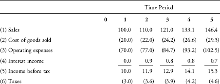
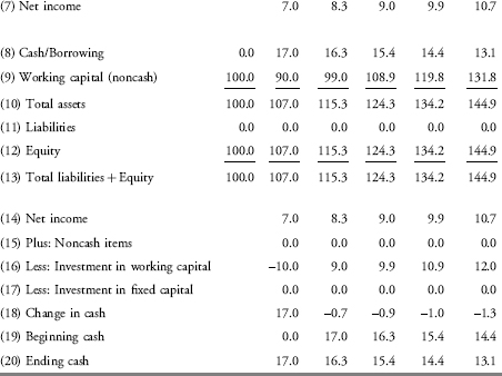
Exhibit 8-4 indicates that at time 0, the company is formed with $100 of equity capital (Line 12). All of the company’s capital is assumed to be immediately invested in working capital (Line 9). In future periods, because it is assumed that no dividends are paid, book equity increases each year by the amount of net income (Line 14). Future periods’ required working capital (Line 9) is assumed to be 90 percent of annual sales (Line 1). Sales are assumed to be $100 in the first period and to grow at a constant rate of 10 percent per year (Line 1). The cost of goods sold is assumed to be constant at 20 percent of sales (Line 2), so the gross profit margin is 80 percent. Operating expenses are assumed to be 70 percent of sales each year (Line 3). Interest income (Line 4) is calculated as 5 percent of the beginning balance of cash/borrowing or the ending balance of the previous period (Line 8) and is an income item when there is a cash balance, as in this example. (If available cash is inadequate to cover required cash outflows, the shortfall is presumed to be covered by borrowing. This borrowing would be shown as a negative balance on Line 8 and an associated interest expense on Line 4. Alternatively, a forecast can be presented with separate lines for cash and borrowing.) Taxes of 30 percent are deducted to obtain net income (Line 7).
To calculate each period’s cash flow, begin with net income (Line 7=Line 14), add back any noncash items, such as depreciation (Line 15), deduct investment in working capital in the period or change in working capital over the period (Line 16), and deduct investment in fixed capital in the period (Line 17).7 In this simple example, we are assuming that the company does not invest in any fixed capital (long-term assets) but, rather, rents furnished office space. Therefore, there is no depreciation and noncash items are zero. Each period’s change in cash (Line 18) is added to the beginning cash balance (Line 19) to obtain the ending cash balance (Line 20=Line 8).
Example 8-5 is simplified to demonstrate some principles of forecasting. In practice, each aspect of a forecast presents a range of challenges. Sales forecasts may be very detailed, with separate forecasts for each year of each product line, each geographical, and/or each business segment. Sales forecasts may be based on past results (for relatively stable businesses), management forecasts, industry studies, and/or macroeconomic forecasts. Similarly, gross profit margins may be based on past results or forecasted relationships and may be detailed. Expenses other than cost of goods sold may be broken down into more detailed line items, each of which may be forecasted on the basis of its relationship with sales (if variable) or on the basis of its historical levels. Working capital requirements may be estimated as a proportion of the amount of sales (as in Example 8-5) or the change in sales or as a compilation of specific forecasts for inventory, receivables, and payables. Most forecasts will involve some investment in fixed assets, in which case, depreciation amounts affect taxable income and net income but not cash flow. Example 8-5 makes the simplifying assumption that interest is paid on the beginning-of-year cash balance.
Example 8-5 develops a series of point estimates for future net income and cash flow. In practice, forecasting generally includes an analysis of the risk in forecasts—in this case, an assessment of the impact on income and cash flow if the realized values of variables differ significantly from the assumptions used in the base case or if actual sales are much different from forecasts. Quantifying the risk in forecasts requires an analysis of the economics of the company’s businesses and expense structure and the potential impact of events affecting the company, the industry, and the economy in general. When that investigation is completed, the analyst can use scenario analysis or Monte Carlo simulation to assess risk. Scenario analysis involves specifying assumptions that differ from those used as the base-case assumptions. In Example 8-5, the projections of net income and cash flow could be recast in a more pessimistic scenario, with assumptions changed to reflect slower sales growth and higher costs. A Monte Carlo simulation involves specifying probability distributions of values for variables and random sampling from those distributions. In the analysis in Example 8-5, the projections would be repeatedly recast with the selected values for the drivers of net income and cash flow, thus permitting the analyst to evaluate a range of possible results and the probability of simulating the possible actual outcomes.
An understanding of financial statements and ratios can enable an analyst to make more detailed projections of income statement, balance sheet, and cash flow statement items. For example, an analyst may collect information on normal inventory and receivables turnover and use this information to forecast accounts receivable, inventory, and cash flows based on sales projections rather than use a composite working capital investment assumption, as in Example 8-5.
As the analyst makes detailed forecasts, he or she must ensure that the forecasts are consistent with each other. For instance, in Example 8-6, the analyst’s forecast concerning days of sales outstanding (which is an estimate of the average time to collect payment from sales made on credit) should flow from a model of the company that yields a forecast of the change in the average accounts receivable balance. Otherwise, predicted days of sales outstanding and accounts receivable will not be mutually consistent.
EXAMPLE 8-6 Consistency of Forecasts8
Brown Corporation had an average days-of-sales-outstanding (DSO) period of 19 days in 2009. An analyst thinks that Brown’s DSO will decline in 2010 (because of expected improvements in the company’s collections department) to match the industry average of 15 days. Total sales (all on credit) in 2009 were $300 million, and Brown expects total sales (all on credit) to increase to $320 million in 2010. To achieve the lower DSO, the change in the average accounts receivable balance from 2009 to 2010 that must occur is closest to:
A. −$3.51 million.
B. −$2.46 million.
C. $2.46 million.
D. $3.51 million.
Solution: B is correct. The first step is to calculate accounts receivable turnover from the DSO collection period. Receivable turnover equals 365/19 (DSO)=19.2 for 2009 and 365/15=24.3 in 2010. Next, the analyst uses the fact that the average accounts receivable balance equals sales/receivable turnover to conclude that for 2009, average accounts receivable was $300,000,000/19.2=$15,625,000 and for 2010, it must equal $320,000,000/24.3=$13,168,724. The difference is a reduction in receivables of $2,456,276.
The next section illustrates the application of financial statement analysis to credit risk analysis.
4. APPLICATION: ASSESSING CREDIT RISK
Credit risk is the risk of loss caused by a counterparty’s or debtor’s failure to make a promised payment. For example, credit risk with respect to a bond is the risk that the obligor (the issuer of the bond) will not be able to pay interest and/or principal according to the terms of the bond indenture (contract). Credit analysis is the evaluation of credit risk. Credit analysis may relate to the credit risk of an obligor in a particular transaction or to an obligor’s overall creditworthiness.
In assessing an obligor’s overall creditworthiness, one general approach is credit scoring, a statistical analysis of the determinants of credit default. Credit analysis for specific types of debt (e.g., acquisition financing and other highly leveraged financing) typically involves projections of period-by-period cash flows.
Whatever the techniques adopted, the analytical focus of credit analysis is on debt-paying ability. Unlike payments to equity investors, payments to debt investors are limited by the agreed contractual interest. If a company experiences financial success, its debt becomes less risky but its success does not increase the amount of payments to its debtholders. In contrast, if a company experiences financial distress, it may be unable to pay interest and principal on its debt obligations. Thus, credit analysis has a special concern with the sensitivity of debt-paying ability to adverse events and economic conditions—cases in which the creditor’s promised returns may be most at risk. Because those returns are generally paid in cash, credit analysis usually focuses on cash flow rather than accrual income. Typically, credit analysts use return measures related to operating cash flow because it represents cash generated internally, which is available to pay creditors.
These themes are reflected in Example 8-7, which illustrates the application to an industry group of four groups of quantitative factors in credit analysis: (1) scale and diversification, (2) tolerance for leverage, (3) operational efficiency, and (4) margin stability.
“Scale and diversification” relate to a company’s sensitivity to adverse events, adverse economic conditions, and other factors—such as market leadership, purchasing power with suppliers, and access to capital markets—that may affect debt-paying ability.
Financial policies, or “tolerance for leverage,” relate to the obligor’s ability to service its indebtedness (i.e., make the promised payments on debt). In Example 8-7, various solvency ratios are used to measure tolerance for leverage. One set of tolerance-for-leverage measures is based on retained cash flow (RCF). RCF is defined by Moody’s Investors Service as operating cash flow before working capital changes less dividends. For example, under the assumption of no capital expenditures, a ratio of RCF to total debt of 0.5 indicates that the company may be able to pay off debt from cash flow retained in the business in approximately 1/0.5=2 years (at current levels of RCF and debt); a ratio adjusting for capital expenditures is also used. Other factors include interest coverage ratios based on EBITDA, which are also chosen by Moody’s in specifying factors for operational efficiency and margin stability.
“Operational efficiency” as defined by Moody’s relates to cost structure: Companies with lower costs are better positioned to deal with financial stress.
“Margin stability” relates to the past volatility of profit margins: Higher stability should be associated with lower credit risk.
EXAMPLE 8-7 Moody’s Evaluation of Quantifiable Rating Factors for a Specific Industry9
Moody’s considers a number of items when assigning credit ratings for the global aerospace and defense industry, including quantitative measures of three broad factors: size and scale; business profile, revenue sustainability, and efficiency; and financial leverage and flexibility. A company’s ratings for each of these factors are weighted and aggregated in determining the overall credit rating assigned. The broad factors, the subfactors, and weightings are as follows:
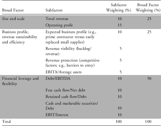
1. What are some reasons why Moody’s may have selected these three broad factors as being important in assigning a credit rating in the aerospace and defense industry?
2. Why might financial leverage and flexibility be weighted so heavily?
Solution to 1:
Size and scale:
- Larger size can strengthen negotiating position with customers and suppliers, leading to better contract terms and potential cost savings.
- Larger scale typically indicates prior success.
- Larger scale can enhance a company’s ability to manage and react to variable market conditions.
- Larger scale often indicates greater geographical, product, and customer diversification.
Business profile, revenue sustainability, and efficiency:
- A business profile that provides some protection from competition, a sustainable flow of revenues as indicated by a strong order backlog, and better operating efficiency should contribute to higher and more sustainable cash flows.
Financial leverage and flexibility:
- Strong financial policies should increase the likelihood of cash flows being sufficient to service debt.
Solution to 2: The level of debt relative to earnings and cash flow is a critical factor in assessing creditworthiness. The higher the current level of debt, the higher the risk of default.
A point to note regarding Example 8-7 is that the rating factors and the metrics used to represent each can vary by industry group. For example, for heavy manufacturing (manufacturing of the capital assets used in other manufacturing and production processes), Moody’s distinguishes order trends and quality as distinctive credit factors affecting future revenues, factory load, and profitability patterns.
Analyses of a company’s historical and projected financial statements are an integral part of the credit evaluation process. As noted by Moody’s, financial statement information is an important source of information for the rating process:
Much of the information used in assessing performance for the subfactors is found in or calculated using the company’s financial statements; others are derived from observations or estimates by the analysts.. . .Moody’s ratings are forward-looking and incorporate our expectations for future financial and operating performance. We use both historical and projected financial results in the rating process. Historical results help us understand patterns and trends for a company’s performance as well as for peer comparison.10
As noted, Moody’ computes a variety of ratios in assessing creditworthiness. A comparison of a company’s ratios with the ratios of its peers is informative in evaluating relative creditworthiness, as demonstrated in Example 8-8.
EXAMPLE 8-8 Peer Comparison of Ratios
A credit analyst is assessing the efficiency and leverage of two aerospace companies on the basis of certain subfactors identified by Moody’s. The analyst collects the information from the companies’ annual reports and calculates the following ratios:11
| Bombardier Inc. | BAE Systems plc | |
| EBITDA/Average assets | 7.5% | 10.1% |
| Debt/EBITDA | 3.9 | 3.1 |
| Retained cash flow to debt | 6.1% | 13.7% |
| Free cash flow to net debt | −7.0% | 7.7% |
Based solely on the data given, which company is more likely to be assigned a higher credit rating, and why?
Solution: The ratio comparisons are all in favor of BAE Systems plc. BAE has a higher level of EBITDA in relation to average assets, higher retained cash flow relative to debt, and higher free cash flow to net debt. BAE also has a lower level of debt relative to EBITDA. Based on the data given, therefore, BAE is likely to be assigned a higher credit rating.
Before calculating ratios such as those presented in Example 8-8, rating agencies make certain adjustments to reported financial statements, such as adjusting debt to include off-balance-sheet debt in a company’s total debt.12 We will describe in Section 6 some common adjustments.
Financial statement analysis, especially financial ratio analysis, can also be an important tool in selecting equity investments, as discussed in the next section.
5. APPLICATION: SCREENING FOR POTENTIAL EQUITY INVESTMENTS
Ratios constructed from financial statement data and market data are often used to screen for potential equity investments. Screening is the application of a set of criteria to reduce a set of potential investments to a smaller set having certain desired characteristics. Criteria involving financial ratios generally involve comparing one or more ratios with some pre-specified target or cutoff values.
A security selection approach incorporating financial ratios may be applied whether the investor uses top-down analysis or bottom-up analysis. Top-down analysis involves identifying attractive geographical segments and/or industry segments, from which the investor chooses the most attractive investments. Bottom-up analysis involves selection of specific investments from all companies within a specified investment universe. Regardless of the direction, screening for potential equity investments aims to identify companies that meet specific criteria. An analysis of this type may be used as the basis for directly forming a portfolio, or it may be undertaken as a preliminary part of a more thorough analysis of potential investment targets.
Fundamental to this type of analysis are decisions about which metrics to use as screens, how many metrics to include, what values of those metrics to use as cutoff points, and what weighting to give each metric. Metrics may include not only financial ratios but also characteristics such as market capitalization or membership as a component security in a specified index. Exhibit 8-5 presents a hypothetical example of a simple stock screen based on the following criteria: a valuation ratio (P/E) less than a specified value, a solvency ratio measuring financial leverage (total debt/assets) not exceeding a specified value, positive net income, and dividend yield (dividends per share divided by price per share) greater than a specified value. Exhibit 8-5 shows the results of applying the screen in August 2010 to a set of 5,187 U.S. companies with market capitalization greater than $100 million, which compose a hypothetical equity manager’s investment universe.
EXHIBIT 8-5 Example of a Stock Screen
Source for data: http://google.com/finance/.
| Stocks Meeting Criterion | ||
| Criterion | Number | Percent of Total |
| P/E <15 | 1,471 | 28.36% |
| Total debt/Assets ≤ 0.5 | 880 | 16.97% |
| Net income/Sales > 0 | 2,907 | 56.04% |
| Dividend yield > 0.5% | 1,571 | 30.29% |
| Meeting all four criteria simultaneously | 101 | 1.95% |
Several points about the screen in Exhibit 8-5 are consistent with many screens used in practice:
- Some criteria serve as checks on the results from applying other criteria. In this hypothetical example, the first criterion selects stocks that appear relatively cheaply valued. The stocks might be cheap for a good reason, however, such as poor profitability or excessive financial leverage. So, the requirement for net income to be positive serves as a check on profitability, and the limitation on financial leverage serves as a check on financial risk. Of course, financial ratios or other statistics cannot generally control for exposure to certain other types of risk (e.g., risk related to regulatory developments or technological innovation).
- If all the criteria were completely independent of each other, the set of stocks meeting all four criteria would be 42, equal to 5,187 times 0.82 percent—the product of the fraction of stocks satisfying the four criteria individually (i.e., 0.2836 × 0.1697 × 0.5604 × 0.3029=0.0082, or 0.82 percent). As the screen illustrates, criteria are often not independent, and the result is that more securities pass the screening than if criteria were independent. In this example, 101 (or 1.95 percent) of the securities pass all four screens simultaneously. For an example of the lack of independence, we note that dividend-paying status is probably positively correlated with the ability to generate positive earnings and the value of the third criterion. If stocks that pass one test tend to also pass another, few are eliminated after the application of the second test.
- The results of screens can sometimes be relatively concentrated in a subset of the sectors represented in the benchmark. The financial leverage criterion in Exhibit 8-5 would exclude banking stocks, for example. What constitutes a high or low value of a measure of a financial characteristic can be sensitive to the industry in which a company operates.
Screens can be used by both growth investors (focused on investing in high-earnings-growth companies), value investors (focused on paying a relatively low share price in relation to earnings or assets per share), and market-oriented investors (an intermediate grouping of investors whose investment disciplines cannot be clearly categorized as value or growth). Growth screens would typically feature criteria related to earnings growth and/or momentum. Value screens, as a rule, feature criteria setting upper limits for the value of one or more valuation ratios. Market-oriented screens would not strongly emphasize valuation or growth criteria. The use of screens involving financial ratios may be most common among value investors.
Many studies have assessed the most effective items of accounting information for screening equity investments. Some research suggests that certain items of accounting information can help explain (and potentially predict) market returns (e.g., Chan et al. 1991; Lev and Thiagarajan 1993; Lakonishok et al. 1994; Davis 1994; Arbanell and Bushee 1998). Representative of such investigations is Piotroski (2000), whose screen uses nine accounting-based fundamentals that aim to identify financially strong and profitable companies among those with high book value/market value ratios. For example, the profitability measures relate to whether the company reported positive net income, positive cash flow, and an increase in return on assets (ROA).
An analyst may want to evaluate how a portfolio based on a particular screen would have performed historically. For this purpose, the analyst uses a process known as “back-testing.” Back-testing applies the portfolio selection rules to historical data and calculates what returns would have been earned if a particular strategy had been used. The relevance of back-testing to investment success in practice, however, may be limited. Haugen and Baker (1996) described some of these limitations:
- Survivorship bias: If the database used in back-testing eliminates companies that cease to exist because of a bankruptcy or merger, then the remaining companies collectively will appear to have performed better.
- Look-ahead bias: If a database includes financial data updated for restatements (where companies have restated previously issued financial statements to correct errors or reflect changes in accounting principles),13 then there is a mismatch between what investors would have actually known at the time of the investment decision and the information used in the back-testing.
- Data-snooping bias: If researchers build a model on the basis of previous researchers’ findings, then use the same database to test that model, they are not actually testing the model’s predictive ability. When each step is backward looking, the same rules may or may not produce similar results in the future. The predictive ability of the model’s rules can validly be tested only by using future data. One academic study has argued that the apparent ability of value strategies to generate excess returns is largely explainable as the result of collective data snooping (Conrad, Cooper, and Kaul, 2003).
EXAMPLE 8-9 Ratio-Based Screening for Potential Equity Investments
Following are two alternative strategies under consideration by an investment firm:
Strategy A: Invest in stocks that are components of a global equity index, have a ROE above the median ROE of all stocks in the index, and have a P/E less than the median P/E.
Strategy B: Invest in stocks that are components of a broad-based U.S. equity index, have a ratio of price to operating cash flow in the lowest quartile of companies in the index, and have shown increases in sales for at least the past three years.
Both strategies were developed with the use of back-testing.
1. How would you characterize the two strategies?
2. What concerns might you have about using such strategies?
Solution to 1: Strategy A appears to aim for global diversification and combines a requirement for high relative profitability with a traditional measure of value (low P/E). Strategy B focuses on both large and small companies in a single market and apparently aims to identify companies that are growing and have a lower price multiple based on cash flow from operations.
Solution to 2: The use of any approach to investment decisions depends on the objectives and risk profile of the investor. With that crucial consideration in mind, we note that ratio-based benchmarks may be an efficient way to screen for potential equity investments. In screening, however, many questions arise.
First, unintentional selections can be made if criteria are not specified carefully. For example, Strategy A might unintentionally select a loss-making company with negative shareholders’ equity because negative net income divided by negative shareholders’ equity arithmetically results in a positive ROE. Strategy B might unintentionally select a company with negative operating cash flow because price to operating cash flow will be negative and thus very low in the ranking. In both cases, the analyst can add additional screening criteria to avoid unintentional selections; these additional criteria could include requiring positive shareholders’ equity in Strategy A and requiring positive operating cash flow in Strategy B.
Second, the inputs to ratio analysis are derived from financial statements, and companies may differ in the financial standards they apply (e.g., IFRS versus U.S. GAAP), the specific accounting method(s) they choose within those allowed by the reporting standards, and/or the estimates made in applying an accounting method.
Third, back-testing may not provide a reliable indication of future performance because of survivorship bias, look-ahead bias, or data-snooping bias. Also, as suggested by finance theory and by common sense, the past is not necessarily indicative of the future.
Fourth, implementation decisions can dramatically affect returns. For example, decisions about frequency and timing of portfolio re-evaluation and changes affect transaction costs and taxes paid out of the portfolio.
6. ANALYST ADJUSTMENTS TO REPORTED FINANCIALS
When comparing companies that use different accounting methods or estimate key accounting inputs in different ways, analysts frequently adjust a company’s financials. In this section, we first provide a framework for considering potential analyst adjustments to facilitate such comparisons and then provide examples of such adjustments. In practice, required adjustments vary widely. The examples presented here are not intended to be comprehensive but, rather, to illustrate the use of adjustments to facilitate a meaningful comparison.
6.1. A Framework for Analyst Adjustments
In this discussion of potential analyst adjustments to a company’s financial statements, we use a framework focused on the balance sheet. Because the financial statements are interrelated, however, adjustments to items reported on one statement may also be reflected in adjustments to items on another financial statement. For example, an analyst adjustment to inventory on the balance sheet affects cost of goods sold on the income statement (and thus also affects net income and, subsequently, the retained earnings account on the balance sheet).
Regardless of the particular order in which an analyst considers the items that may require adjustment for comparability, the following aspects are appropriate:
- Importance (materiality): Is an adjustment to this item likely to affect the conclusions? In other words, does it matter? For example, in an industry where companies require minimal inventory, does it matter that two companies use different inventory accounting methods?
- Body of standards: Is there a difference in the body of standards being used (U.S. GAAP versus IFRS)? If so, in which areas is the difference likely to affect a comparison?
- Methods: Is there a difference in accounting methods used by the companies being compared?
- Estimates: Is there a difference in important estimates used by the companies being compared?
The following sections illustrate analyst adjustments—first, those relating to the asset side of the balance sheet and then those relating to the liability side.
6.2. Analyst Adjustments Related to Investments
Accounting for investments in the debt and equity securities of other companies (other than investments accounted for under the equity method and investments in consolidated subsidiaries) depends on management’s intention (i.e., whether to actively trade the securities, make them available for sale, or in the case of debt securities, hold them to maturity). When securities are classified as “financial assets measured at fair value through profit or loss” (similar to “trading” securities in U.S. GAAP), unrealized gains and losses are reported in the income statement. When securities are classified as “financial assets measured at fair value through other comprehensive income” (similar to “available-for-sale” securities in U.S. GAAP), unrealized gains and losses are not reported in the income statement and, instead, are recognized in equity. If two otherwise comparable companies have significant differences in the classification of investments, analyst adjustments may be useful to facilitate comparison.
6.3. Analyst Adjustments Related to Inventory
With inventory, adjustments may be required for different accounting methods. As described in previous readings, a company’s decision about inventory method will affect the value of inventory shown on the balance sheet as well as the value of inventory that is sold (cost of goods sold). If a company not reporting under IFRS14 uses LIFO (last-in, first-out) and another uses FIFO (first-in, first-out), comparability of the financial results of the two companies will suffer. Companies that use the LIFO method, must also, however, disclose the value of their inventory under the FIFO method. To recast inventory values for a company using LIFO reporting on a FIFO basis, the analyst adds the ending balance of the LIFO reserve to the ending value of inventory under LIFO accounting. To adjust cost of goods sold to a FIFO basis, the analyst subtracts the change in the LIFO reserve from the reported cost of goods sold under LIFO accounting. Example 8-10 illustrates the use of a disclosure of the value of inventory under the FIFO method to make a more consistent comparison of the current ratios of two companies reporting in different methods.
EXAMPLE 8-10 Adjustment for a Company Using LIFO Accounting for Inventories
An analyst is comparing the financial performance of Carpenter Technology Corporation (NYSE: CRS), a U.S. company operating in the specialty metals industry, with the financial performance of a similar company that uses IFRS for reporting. Under IFRS, this company uses the FIFO method of inventory accounting. Therefore, the analyst must convert results to a comparable basis. Exhibit 8-6 provides balance sheet information on CRS.
EXHIBIT 8-6 Data for Carpenter Technology Corporation
Source: 10-K for Carpenter Technology Corporation for the year ended 30 June 2010.
| 30 June | ||
| 2010 | 2009 | |
| Total current assets | 820.2 | 749.7 |
| Total current liabilities | 218.1 | 198.5 |
| NOTE 6. INVENTORIES | ||
| Inventories consist of the following ($ millions): | ||
| 30 June | ||
| 2010 | 2009 | |
| Raw materials | $30.7 | $29.5 |
| Work in process | 109.1 | 90.8 |
| Finished goods | 63.8 | 65.1 |
| $203.6 | $185.4 | |
| If the first-in, first-out method of inventory had been used instead of the LIFO method, inventories would have been $331.8 and $305.8 million higher as of June 30, 2010 and 2009, respectively. | ||
1. Based on the information in Exhibit 8-6, calculate CRS’s current ratio under FIFO and LIFO for 2009 and 2010.
2. CRS makes the following disclosure in the risk section of its MD&A. Assuming an effective tax rate of 35 percent, estimate the impact on CRS’s tax liability.
“We value most of our inventory using the LIFO method, which could be repealed resulting in adverse affects on our cash flows and financial condition.
The cost of our inventories is primarily determined using the Last-In First-Out (“LIFO”) method. Under the LIFO inventory valuation method, changes in the cost of raw materials and production activities are recognized in cost of sales in the current period even though these materials and other costs may have been incurred at significantly different values due to the length of time of our production cycle. Generally in a period of rising prices, LIFO recognizes higher costs of goods sold, which both reduces current income and assigns a lower value to the year-end inventory. Recent proposals have been initiated aimed at repealing the election to use the LIFO method for income tax purposes. According to these proposals, generally taxpayers that currently use the LIFO method would be required to revalue their LIFO inventory to its first-in, first-out (“FIFO”) value. As of June 30, 2010, if the FIFO method of inventory had been used instead of the LIFO method, our inventories would have been about $332 million higher. This increase in inventory would result in a one time increase in taxable income which would be taken into account ratably over the first taxable year and the following several taxable years. The repeal of LIFO could result in a substantial tax liability which could adversely impact our cash flows and financial condition.”
Source: 10-K for Carpenter Technology Corporation for the year ended 30 June 2010.
3. CRS reported cash flow from operations of $115.2 million for the year ended 30 June 2010. In comparison with the company’s operating cash flow, how significant is the additional potential tax liability?
Solution to 1: The calculations of CRS’s current ratio (current assets divided by current liabilities) are as follows:
| 2010 | 2009 | |
| I. Current ratio (unadjusted) | ||
| Total current assets | $820.2 | $749.7 |
| Total current liabilities | $218.1 | $198.5 |
| Current ratio (unadjusted) | 3.8 | 3.8 |
| II. Current ratio (adjusted) | ||
| Total current assets | $820.2 | $749.7 |
| Adjust inventory to FIFO, add: | 331.8 | 305.8 |
| Total current assets (adjusted) | $1,152 | $1,056 |
| Total current liabilities | 218.1 | 198.5 |
| Current ratio (adjusted) | 5.3 | 5.3 |
To adjust the LIFO inventory to FIFO, add the excess amounts of FIFO cost over LIFO cost to LIFO inventory and increase current assets by an equal amount. The effect of adjusting inventory on the current ratio is to increase the current ratio from 3.8 to 5.3 in both 2009 and 2010. CRS has greater liquidity according to the adjusted current ratio.
Solution to 2: Assuming an effective tax rate of 35 percent, we find the total increase in CRS’s tax liability to be $116.1 million (0.35 × $331.8 million).
Solution to 3: The additional tax liability would be greater than the entire amount of the company’s cash flow from operations of $115.2 million; the additional tax liability would be apportioned, however, over several years.
In summary, the information disclosed by companies that use LIFO allows an analyst to calculate the value of the company’s inventory as if the company were using the FIFO method. In Example 8-10, the portion of inventory valued under the LIFO method was a relatively small portion of total inventory; the LIFO reserve (excess of FIFO cost over LIFO) was also relatively small. If the LIFO method is used for a substantial part of a company’s inventory and the LIFO reserve is large relative to reported inventory, however, the adjustment to a FIFO basis can be important for comparison of the LIFO-reporting company with a company that uses the FIFO method of inventory valuation. Example 8-11 illustrates a case in which such an adjustment would have a major impact on an analyst’s conclusions.
EXAMPLE 8-11 Analyst Adjustment to Inventory Value for Comparability in a Current Ratio Comparison
Company A reports under IFRS and uses the FIFO method of inventory accounting. Company B reports under U.S. GAAP and uses the LIFO method. Exhibit 8-7 gives data pertaining to current assets, LIFO reserves, and current liabilities of these companies.
EXHIBIT 8-7 Data for Companies Accounting for Inventory on Different Bases
| Company A (FIFO) | Company B (LIFO) | |
| Current assets (includes inventory) | $300,000 | $80,000 |
| LIFO reserve | NA | $20,000 |
| Current liabilities | $150,000 | $45,000 |
NA=not applicable.
Based on the data given in Exhibit 8-7, compare the liquidity of the two companies as measured by the current ratio.
Solution: Company A’s current ratio is 2.0. Based on unadjusted balance sheet data, Company B’s current ratio is 1.78. Company A’s higher current ratio indicates that Company A appears to be more liquid than Company B; however, the use of unadjusted data for Company B is not appropriate for making comparisons with Company A.
After adjusting Company B’s inventory to a comparable basis (i.e., to a FIFO basis), the conclusion changes. The following table summarizes the results when Company B’s inventory is left on a LIFO basis and when it is placed on a FIFO basis for comparability with Company A.
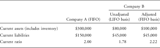
When both companies’ inventories are stated on a FIFO basis, Company B appears to be the more liquid, as indicated by its current ratio of 2.22 versus Company A’s ratio of 2.00.
The adjustment to place Company B’s inventory on a FIFO basis was significant because Company B was assumed to use LIFO for its entire inventory and its inventory reserve was $20,000/$80,000=0.25, or 25 percent of its reported inventory.
As mentioned earlier, an analyst can also adjust the cost of goods sold for a company using LIFO to a FIFO basis by subtracting the change in the amount of the LIFO reserve from cost of goods sold. Such an adjustment would be appropriate for making profitability comparisons with a company reporting on a FIFO basis and is important to make when the impact of the adjustment would be material.
6.4. Analyst Adjustments Related to Property, Plant, and Equipment
Management generally has considerable discretion in determination of depreciation expense. Depreciation expense affects the values of reported net income and reported net fixed assets. Analysts often consider management’s choices related to depreciation as a qualitative factor in evaluating the quality of a company’s financial reporting, and in some cases, analysts may adjust reported depreciation expense for a specific analytical purpose.
The amount of depreciation expense depends on both the accounting method and the estimates used in the calculations. Companies can use the straight-line method, an accelerated method, or a usage method to depreciate fixed assets (other than land). The straight-line method reports an equal amount of depreciation expense each period, and the expense is computed as the depreciable cost divided by the estimated useful life of the asset (when acquired, an asset’s depreciable cost is calculated as its total cost minus its estimated salvage value). Accelerated methods depreciate the asset more quickly; they apportion a greater amount of the depreciable cost to depreciation expense in the earlier periods. Usage-based methods depreciate an asset in proportion to its usage. In addition to selecting a depreciation method, companies must estimate an asset’s salvage value and useful life to compute depreciation.
Disclosures required for depreciation often do not facilitate specific adjustments, so comparisons of companies concerning their decisions in depreciating assets are often qualitative and general. The accounts that are associated with depreciation include the balance sheet accounts for gross property, plant, and equipment (PPE) and accumulated depreciation; the income statement amount for depreciation expense; and the statement of cash flows disclosure of capital expenditure (capex) and asset disposals. The relationships among these items can reveal various pieces of information. Note, however, that PPE typically includes a mix of assets with different depreciable lives and salvage values, so the items in the following list reflect general relationships in the total pool of assets.
- Accumulated depreciation divided by gross PPE, from the balance sheet, suggests how much of the useful life of the company’s overall asset base has passed.
- Accumulated depreciation divided by depreciation expense suggests how many years’ worth of depreciation expense have already been recognized (i.e., the average age of the asset base).
- Net PPE (net of accumulated depreciation) divided by depreciation expense is an approximate indicator of how many years of useful life remain for the company’s overall asset base.
- Gross PPE divided by depreciation expense suggests the average life of the assets at installation.
- Capex divided by the sum of gross PPE plus capex can suggest what percentage of the asset base is being renewed through new capital investment.
- Capex in relation to asset disposal provides information on growth of the asset base.
As Example 8-12 shows, these relationships can be evaluated for companies in an industry to suggest differences in their strategies for asset utilization or areas for further investigation.
EXAMPLE 8-12 Differences in Depreciation
An analyst is evaluating the financial statements of two companies in the same industry. The companies have similar strategies with respect to the use of equipment in manufacturing their products. The following information is provided (amounts in millions):
| Company A | Company B | |
| Net PPE | $1,200 | $750 |
| Depreciation expense | $120 | $50 |
1. Based on the information given, estimate the average remaining useful lives of the asset bases of Company A and Company B.
2. Suppose that, based on a physical inspection of the companies’ plants and other industry information, the analyst believes that the actual remaining useful lives of Company A’s and Company B’s assets are roughly equal at 10 years. Based only on the facts given, what might the analyst conclude about Company B’s reported net income?
Solution to 1: The estimated average remaining useful life of Company A’s asset base is 10 years (calculated as net PPE divided by depreciation expense, or $1,200/$120=10 years). For Company B, the average remaining useful life of the asset base appears to be far longer, 15 years ($750/$50).
Solution to 2: If 10 years were used to calculate Company B’s depreciation expense, the expense would be $75 million (i.e., $25 million higher than reported) and higher depreciation expense would decrease net income. The analyst might conclude that Company B’s reported net income reflects relatively more aggressive accounting estimates than estimates reflected in Company A’s reported net income.
6.4. Analyst Adjustments Related to Goodwill
Goodwill arises when one company purchases another for a price that exceeds the fair value of the net identifiable assets acquired. Net identifiable assets include current assets, fixed assets, and certain intangible assets that have value and meet recognition criteria under accounting standards. A broad range of intangible assets might require valuation in the context of a business combination—for example, brands, technology, and customer lists. Goodwill is recorded as an asset and essentially represents the difference between the purchase price and the net identifiable assets. For example, assume ParentCo purchases TargetCo for a purchase price of $400 million and the fair value of TargetCo’s identifiable assets is $300 million (which includes the fair values of current assets, fixed assets, and a recognized brand). ParentCo will record total assets of $400 million consisting of $300 million in identifiable assets (including the fair value of the brand) and $100 million of goodwill. The goodwill is tested annually for impairment and if the value of the goodwill is determined to be impaired, ParentCo will then reduce the amount of the asset and report a write-off resulting from impairment.
One of the conceptual difficulties with goodwill arises in comparative financial statement analysis. Consider, for example, two hypothetical U.S. companies, one of which has grown by making an acquisition and the other of which has grown internally. Assume that the economic value of the two companies is identical: Each has an identically valuable branded product, well-trained workforce, and proprietary technology. The company that has grown by acquisition will have recorded the transaction to acquire the target company and its underlying net assets on the basis of the total consideration paid for the acquisition. The company that has grown internally will have done so by incurring expenditures for advertising, staff training, and research, all of which are expensed as incurred under U.S. GAAP. Given the immediate expensing, the value of the internally generated assets is not capitalized onto the balance sheet and is thus not directly reflected on the company’s balance sheet (revenues, income, and cash flows should reflect the benefits derived from the investment in the intangible assets). Ratios based on asset values and/or income, including profitability ratios (such as ROA) and market value to book value (MV/BV),15will generally differ for the two companies because of differences in the accounting values of assets and income related to acquired intangibles and goodwill, although, by assumption, the economic value of the companies is identical.
EXAMPLE 8-13 Ratio Comparisons for Goodwill
Miano Marseglia is an analyst who is evaluating the relative valuation of two securities brokerage companies: TD Ameritrade Holding Corporation (NasdaqGS: AMTD) and the Charles Schwab Corporation (NYSE: SCHW). As one part of an overall analysis, Marseglia would like to see how the two companies compare with each other and with the industry based on market value to book value. Because both companies are large players in the industry, Marseglia expects them to sell at a higher MV/BV than the industry median of 1.2. He collects the following data on the two companies.
| SCHW | AMTD | |
| Market capitalization on January 2010 (market price per share times the number of shares outstanding) | $21,871 | $11,525 |
| Total shareholders’ equity as of most recent quarter | $5,073 | $3,551 |
| Goodwill | $528 | $2,472 |
| Other intangible assets | $23 | $1,225 |
Marseglia computes the MV/BV for the companies as follows:
SCHW $21,871/$5,073=4.3
AMTD $11,525/$3,551=3.2
As expected, each company appears to be selling at a premium to the industry average MV/BV of 1.2. The companies have similar MV/BVs (i.e., they are somewhat equally valued relative to the book value of shareholders’ equity), but based solely on MV/BV, AMTD appears to be a better value. Marseglia is concerned, however, because he notes that AMTD has significant amounts of goodwill and acquired intangible assets. He wonders what the relative value would be if the MV/BV were computed after adjusting book value, first, to remove goodwill and, second, to remove all intangible assets. Book value reduced by all intangible assets (including goodwill) is known as “tangible book value.” The median price/tangible book value for the industry is 1.3.
1. Compute the MV/BV adjusted for goodwill and the price/tangible book value for each company.
2. Which company appears to be a better value based solely on this data? (Note that the MV/BV is only one part of a broader analysis. Much more evidence related to the valuations and the comparability of the companies would be required to reach a conclusion about whether one company is a better value.)
Solution to 1:
| ($ millions) | ||
| SCHW | AMTD | |
| Total stockholders’ equity | $5,073 | $3,551 |
| Less: Goodwill | $528 | $2,472 |
| Book value, adjusted | $4,545 | $1,079 |
| Adjusted MV/BV | 4.8 | 10.7 |
| ($ millions) | ||
| SCHW | AMTD | |
| Total stockholders’ equity | $5,073 | $3,551 |
| Less: Goodwill | $528 | $2,472 |
| Less: Other intangible assets | $23 | $1,225 |
| Tangible book value | $4,522 | ($146) |
| MV/tangible book value | 4.8 | NM |
NM=not meaningful.
Solution to 2: After adjusting for goodwill, SCHW appears to be selling for a lower price relative to book value than does AMTD (4.8 versus 10.7). Both companies are selling at a premium to the industry, particularly AMTD, after adjusting for goodwill.
SCHW is also selling for a higher multiple than the industry (4.8 versus 1.3) based on price/tangible book value. AMTD has a negative tangible book value and, therefore, its price/tangible book value is not meaningful. Based on this interpretation and based solely on this information, Marseglia would conclude that AMTD is relatively more expensive than SCHW.
6.6. Analyst Adjustments Related to Off-Balance-Sheet Financing
A number of business activities give rise to obligations that, although they are economically liabilities of a company, are not required to be reported on a company’s balance sheet. Including such off-balance-sheet obligations in a company’s liabilities can affect ratios and conclusions based on such ratios. In this section, we describe adjustments to financial statements related to one type of off-balance-sheet obligation, the operating lease. (Note that revised leasing standards proposed in 2011 eliminate the existing operating lease distinction; if implemented, these standards are likely to change or even eliminate adjustments required for operating leases.)
The rights of a lessee (the party that is leasing some asset) may be similar to the rights of an owner, but if the terms of the lease can be structured so it can be accounted for as an operating lease, the lease is treated like a rental contract and neither the leased asset nor the associated liability is reported on the balance sheet.16 The lessee simply records the periodic lease payment as a rental expense in its income statement. In contrast, when a company actually owns an asset, the asset is shown on the balance sheet, together with any corresponding liability, such as financing for the asset. Similarly, if a lease is accounted for as a capital lease—essentially equivalent to ownership—the leased asset and associated liability appear on the lessee’s balance sheet.
What is of concern to analysts is when a lease conveys to the lessee most of the benefits and risks of ownership but the lease is accounted for as an operating lease—giving rise to off-balance-sheet financing. International accounting standard setters have stated that the entities should not avoid balance sheet recording of leases through artificial leasing structures.
A 2005 report by the U.S. SEC on off-balance-sheet financing estimates that more than 63 percent of companies in the United States report having an operating lease. The SEC estimate of total future lease payments under operating leases was $1.2 trillion over the remaining terms of the leases.
Because companies are required to disclose in their financial statements the amount and timing of lease payments, an analyst can use this information to answer the question: How would a company’s financial position look if operating lease obligations were included in its total liabilities?
Exhibit 8-8 presents selected items from the balance sheet of AMR Corporation (the parent of American Airlines) and the text of the footnote from the financial statements about the company’s leases. We use the information in this exhibit to illustrate analyst adjustments.
EXHIBIT 8-8 Lease Arrangements of AMR Corporation (NYSE: AMR)—Selected Items from Balance Sheet ($ millions)
Source: AMR Corporation’s Form 10-K for period ending 31 December 2009.
| 31 December | ||
| 2009 | 2008 | |
| Total Assets | $25,438 | $25,175 |
| Current maturities of long-term debt | $1,024 | $1,845 |
| Long-term debt, less current maturities | 9,984 | 8,423 |
| Total long-term debt | 11,008 | 10,268 |
| Current obligations under capital leases | 90 | 107 |
| Obligations under capital leases, less current obligations | 599 | 582 |
| Total long-term debt and capital leases | $11,697 | $10,957 |
| From FOOTNOTE 5. LEASES | ||
| AMR’s subsidiaries lease various types of equipment and property, primarily aircraft and airport facilities. The future minimum lease payments required under capital leases, together with the present value of such payments, and future minimum lease payments required under operating leases that have initial or remaining noncancellable lease terms in excess of one year as of December 31, 2009, were (in millions): | ||
| Capital | Operating | |
| Year Ending December 31 | Leases | Leases |
| 2010 | $181 | $1,057 |
| 2011 | 184 | 1,032 |
| 2012 | 134 | 848 |
| 2013 | 119 | 755 |
| 2014 | 98 | 614 |
| 2015 and thereafter | 436 | 5,021 |
| $1,152 | $9,327(1) | |
| Less amount representing interest | 463 | |
| Present value of net minimum lease payments | $689 | |
(1) As of December 31, 2009, included in Accrued liabilities and Other liabilities and deferred credits on the accompanying consolidated balance sheet is approximately $1.2 billion relating to rent expense being recorded in advance of future operating lease payments.
To evaluate the company’s solvency, we can calculate the debt-to-assets ratio, defined as the ratio of total debt to total assets. When we include obligations under capital leases (amounting to $689 million in 2009), the debt-to-assets ratio for 2009 is 46.0 percent (total long-term debt/total assets=$11,697/$25,438). The company’s footnote on leases discloses a total of $9.3 billion of future payments for operating leases on an undiscounted basis. The footnote also indicates that of this amount, only $1.2 billion is shown on the balance sheet. To determine the impact of including operating lease obligations in total liabilities, we can calculate the present value of the future operating lease payments. Calculating the present value of these payments requires a discount rate. We can estimate an appropriate discount rate from the information about the present value of the capital lease payments. Using the present value of the capital lease payments and the schedule of future payments, we can calculate the internal rate of return (i.e., the return that results in the discounted future payments equaling the present value). The internal rate of return from the capital lease information can then be used as the discount rate to estimate the present value of the series of operating lease payments.
For AMR, the present value of the capital lease payments is $689 million. Exhibit 8-9 shows different assumed streams of payments based on the information given in the footnote and illustrates the sensitivity of the analysis to assumptions about the timing of cash flows. Each assumed stream results in a different implied discount rate on the lease or internal rate of return to the lease. Using the stream of payments shown in the footnote and assuming that all of the $436 million payments indicated for 2015 and thereafter are made in the year 2015 results in an internal rate of return of 15.04 percent. Based on the schedule of payments shown, a more reasonable assumption, however, is that the $436 million payments do not all occur in a single year. One approach to estimating the timing of these payments is to assume that the payments in 2015 and subsequent years equal the average annual payments in years 2010–2014 of $143=($181+$184+$134+$119+$98)/5. Using this approach, we assume payments in 2015 and the following three years that total the amount shown in the footnote for 2015 and the internal rate of return of the capital lease is 13.90 percent. Given that lease payments have been generally declining over 2010–2015, another approach is to assume that the amount of the lease payment after 2015 remains constant in subsequent years at an amount equal to the payment in 2014 until the total amount shown in the note for 2015 is reached. Using this assumption, we find the internal rate of return of the capital lease payments is 13.24 percent.17
We developed discount rate estimates of 13.90 percent and 13.24 percent. Using a discount rate of 13.90 percent, the present value of future operating lease payments would be roughly $5.5 billion, and using a discount rate of 13.24 percent, the present value would be around $5.6 billion. Because $1.2 billion of the amounts related to operating leases already appear on the balance sheet (as disclosed in the company’s lease footnote), the value of the future operating lease payments that do not appear on the balance sheet are estimated to be in the range of $5,466 million − $1,200 million=$4,266 million to $5,632 million − $1,200 million=$4,432 million. The lower the assumed discount rate, the higher the present value of the lease payments.
EXHIBIT 8-9 Present Value of Operating Lease Payments Using a Discount Rate Derived from Present Value of Capital Lease Payments ($ millions)
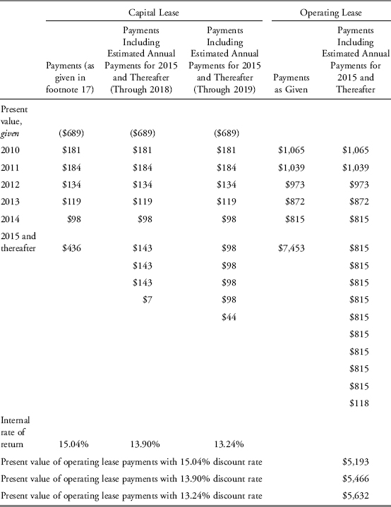
We now add the present value of the off-balance-sheet future operating lease payments to the company’s total assets and total debt. Making this adjustment increases the debt-to-assets ratio to an amount between ($11,697+$4,266)/($25,438+$4,266)=67.5 percent and ($11,697+$4,432)/($25,438+$4,432)=68.1 percent. The discount rates implied by the company’s capital lease structure are significantly higher, however, than yields on investment-grade bonds as of the date of the example; therefore, an analyst might choose to examine the sensitivity of the lease obligation to alternative discount rates.
EXAMPLE 8-14 Analyst Adjustment to Debt for Operating Lease Payments
An analyst is evaluating the capital structure of two (hypothetical) companies, Koller Semiconductor and MacRae Manufacturing, as of the beginning of 2010. Koller Semiconductor makes somewhat less use of operating leases than MacRae Manufacturing. The analyst has the additional information in Exhibit 8-10.
| Koller Semiconductor | MacRae Manufacturing | |
| Total debt | $1,200 | $2,400 |
| Total equity | $2,000 | $4,000 |
| Average interest rate on debt | 10% | 8% |
| Lease payments on operating leases: | ||
| 2010 | 10 | 90 |
| 2011 | 18 | 105 |
| 2012 | 22 | 115 |
| 2013 | 25 | 128 |
| 2014 and thereafter | 75 | 384 |
Based on the information given in Exhibit 8-10 and assuming no adjustment to equity, discuss how adjusting for operating leases affects the companies’ solvency on the basis of debt/debt-plus-equity. (Assume payments after 2013 occur at the same rate as for 2013. For example, for Koller Semiconductor, the payments for 2014 through 2016 would be assumed to be $25 each year.)
Solution: Before the adjustment is made, the companies’ debt/debt-plus-equity are identical, both at 37.5 percent. To make the adjustment for operating leases, the first step is to calculate the present value of the operating lease payments. Assuming that payments after 2013 occur at the same rate as for 2013, the analyst finds Koller’s payment would be $25 in 2014, 2015, and 2016. The present value of $25 discounted for five years at 10 percent is $15.52. MacRae’s payment is assumed to be $128 in each of 2014, 2015, and 2016. The present value of $128 discounted for five years at 8 percent is $87.11. Calculations for 2015 and 2016 are made in the same manner, resulting in the present values shown in Exhibit 8-11.
| Koller Semiconductor | MacRae Manufacturing | |
| 2010 | $9.09 | $83.33 |
| 2011 | $14.88 | $90.02 |
| 2012 | $16.53 | $91.29 |
| 2013 | $17.08 | $94.08 |
| 2014 | $15.52 | $87.11 |
| 2015 | $14.11 | $80.66 |
| 2016 | $12.83 | $74.69 |
| Total present value | $100.04 | $601.18 |
After the present value of capitalized lease obligations is added to total debt, MacRae Manufacturing’s debt/debt-plus-equity is significantly higher, at 42.9 percent, than the debt/debt-plus-equity of Koller Semiconductor, as shown in Exhibit 8-12. The higher ratio reflects the impact of lease obligations on MacRae’s solvency, as measured by debt/debt-plus-equity.
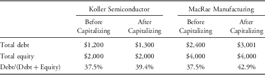
The adjustment for operating leases essentially treats the transaction as if the asset subject to the operating lease had been purchased rather than leased. The present value of the capitalized lease obligations is the amount owed and the amount at which the asset is valued. Further adjustments reflect the reduction of rent expenses (if the asset is owned, rent would not be paid), the related interest expense on the amount owed, and a depreciation expense for the asset. The reduction of rent expense can be estimated as the average of two years of rent expense. Interest expense is estimated as the interest rate times the present value of the lease payments. Depreciation is estimated on a straight-line basis for the number of years of future lease payments.
EXAMPLE 8-15 Effect on Coverage Ratio for Operating Lease Adjustment
The analyst is also evaluating the interest coverage ratio of the companies in the previous example, Koller Semiconductor and MacRae Manufacturing.
| Koller Semiconductor | MacRae Manufacturing | |
| EBIT before adjustment | $850 | $1,350 |
| Interest expense before adjustment | $120 | $192 |
The prior-year (2009) rent expense was $11 for Koller Semiconductor and $90 for MacRae Manufacturing.
Using the information in Example 8-14 and the additional information given here, discuss how adjustment for operating leases affects the companies’ solvency as measured by their coverage ratios.
Solution: Interest coverage is calculated as EBIT divided by interest. For the adjustments, rent expense is the average of two years of rent. For Koller Semiconductor, rent expense is calculated as ($11+$10)/2. The cost of interest on lease obligations is estimated as the interest rate multiplied by the present value of the lease payments. For Koller Semiconductor, this interest expense is calculated as 10% × $100.04, and for MacRae Manufacturing, it is calculated as 8% × $601.18. Depreciation is estimated on a straight-line basis by dividing the present value of lease payments by the number of years of lease payments (seven years). After the adjustment, both companies show a decline in interest coverage ratio, reflecting the increased obligation associated with the operating leases (Exhibit 8-13). Also the apparent difference in the coverage between the two companies is larger than it was in Example 8-12.
| Koller Semiconductor | MacRae Manufacturing | |
| Interest coverage before adjustment | 7.1 | 7.0 |
| EBIT before adjustment | $850.0 | $1,350.0 |
| Rent expense (an add-back to EBIT) | 10.5 | 90.0 |
| Depreciation (a deduction from EBIT) | (14.3) | (85.9) |
| EBIT after adjustment | $846.2 | $1354.1 |
| Interest expense before adjustment | $120.0 | $192.0 |
| Assumed cost of interest on lease obligation (to add to interest) | 10.0 | 48.1 |
| Interest expense after adjustment | $130.0 | $240.1 |
| Interest coverage after adjustment | 6.5 | 5.6 |
In summary, adjusting a company’s financial statements to include amounts of lease payments provides a more complete picture of the company’s financial condition and enables the comparison of companies with varying arrangements for financing assets. The analyst may also need to adjust for amounts associated with other off-balance-sheet financing arrangements.
This reading described selected applications of financial statement analysis, including the evaluation of past financial performance, the projection of future financial performance, the assessment of credit risk, and the screening of potential equity investments. In addition, the reading introduced analyst adjustments to reported financials. In all cases, the analyst needs to have a good understanding of the financial reporting standards under which the financial statements were prepared. Because standards evolve over time, analysts must stay current in order to make good investment decisions.
The main points in the reading are as follows:
- Evaluating a company’s historical performance addresses not only what happened but also the causes behind the company’s performance and how the performance reflects the company’s strategy.
- The projection of a company’s future net income and cash flow often begins with a top-down sales forecast in which the analyst forecasts industry sales and the company’s market share. By projecting profit margins or expenses and the level of investment in working and fixed capital needed to support projected sales, the analyst can forecast net income and cash flow.
- Projections of future performance are needed for discounted cash flow valuation of equity and are often needed in credit analysis to assess a borrower’s ability to repay interest and principal of a debt obligation.
- Credit analysis uses financial statement analysis to evaluate credit-relevant factors, including tolerance for leverage, operational stability, and margin stability.
- When ratios constructed from financial statement data and market data are used to screen for potential equity investments, fundamental decisions include which metrics to use as screens, how many metrics to include, what values of those metrics to use as cutoff points, and what weighting to give each metric.
- Analyst adjustments to a company’s reported financial statements are sometimes necessary (e.g., when comparing companies that use different accounting methods or assumptions). Adjustments include those related to investments; inventory; property, plant, and equipment; goodwill; and off-balance-sheet financing.
1. Projecting profit margins into the future on the basis of past results would be most reliable when the company:
A. is in the commodities business.
B. operates in a single business segment.
C. is a large, diversified company operating in mature industries.
2. Galambos Corporation had an average receivables collection period of 19 days in 2003. Galambos has stated that it wants to decrease its collection period in 2004 to match the industry average of 15 days. Credit sales in 2003 were $300 million, and analysts expect credit sales to increase to $400 million in 2004. To achieve the company’s goal of decreasing the collection period, the change in the average accounts receivable balance from 2003 to 2004 that must occur is closest to:
A. −$420,000.
B. $420,000.
C. $836,000.
3. Credit analysts are likely to consider which of the following in making a rating recommendation?
A. Business risk but not financial risk
B. Financial risk but not business risk
C. Both business risk and financial risk
4. When screening for potential equity investments based on return on equity, to control risk, an analyst would be most likely to include a criterion that requires:
A. positive net income.
B. negative net income.
C. negative shareholders’ equity.
5. One concern when screening for stocks with low price-to-earnings ratios is that companies with low P/Es may be financially weak. What criterion might an analyst include to avoid inadvertently selecting weak companies?
A. Net income less than zero
B. Debt-to-total assets ratio below a certain cutoff point
C. Current-year sales growth lower than prior-year sales growth
6. When a database eliminates companies that cease to exist because of a merger or bankruptcy, this can result in:
A. look-ahead bias.
B. back-testing bias.
C. survivorship bias.
7. In a comprehensive financial analysis, financial statements should be:
A. used as reported without adjustment.
B. adjusted after completing ratio analysis.
C. adjusted for differences in accounting standards, such as international financial reporting standards and U.S. generally accepted accounting principles.
8. When comparing financial statements prepared under IFRS with those prepared under U.S. GAAP, analysts may need to make adjustments related to:
A. realized losses.
B. unrealized gains and losses for trading securities.
C. unrealized gains and losses for available-for-sale securities.
9. When comparing a U.S. company that uses the last in, first out (LIFO) method of inventory with companies that prepare their financial statements under international financial reporting standards (IFRS), analysts should be aware that according to IFRS, the LIFO method of inventory:
A. is never acceptable.
B. is always acceptable.
C. is acceptable when applied to finished goods inventory only.
10. An analyst is evaluating the balance sheet of a U.S. company that uses last in, first out (LIFO) accounting for inventory. The analyst collects the following data:
| 31 Dec 05 | 31 Dec 06 | |
| Inventory reported on balance sheet | $500,000 | $600,000 |
| LIFO reserve | $50,000 | $70,000 |
| Average tax rate | 30% | 30% |
After adjusting the amounts to convert to the first in, first out (FIFO) method, inventory at 31 December 2006 would be closest to:
A. $600,000.
B. $620,000.
C. $670,000.
11. An analyst gathered the following data for a company ($millions):
| 31 Dec 2000 | 31 Dec 2001 | |
| Gross investment in fixed assets | $2.8 | $2.8 |
| Accumulated depreciation | $1.2 | $1.6 |
The average age and average depreciable life of the company’s fixed assets at the end of 2001 are closest to:
| Average Age | Average Depreciable Life |
| A. 1.75 years | 7 years |
| B. 1.75 years | 14 years |
| C. 4.00 years | 7 years |
12. To compute tangible book value, an analyst would
A. add goodwill to stockholders’ equity.
B. add all intangible assets to stockholders’ equity.
C. subtract all intangible assets from stockholders’ equity.
13. Which of the following is an off-balance-sheet financing technique? The use of
A. capital leases.
B. operating leases.
C. the last in, first out inventory method.
14. To better evaluate the solvency of a company, an analyst would most likely add to total liabilities
A. the present value of future capital lease payments.
B. the total amount of future operating lease payments.
C. the present value of future operating lease payments.
1Pinto et al. (2010) describe market-based valuation as using price multiples—ratios of a stock’s market price to some measure of value per share (e.g., price-to-earnings ratios). Although the valuation method may be used independently of an analysis of a company’s past financial performance, such an analysis may provide reasons for differences in companies’ price multiples.
2Pownall and Schipper (1999).
3In a study of European companies’ reconciliations in the last year that reconciliations were required by the SEC, Henry, Lin, and Yang (2009) found that most of the companies reported IFRS net income higher than U.S. GAAP net income and reported IFRS shareholders’ equity lower than U.S. GAAP shareholders’ equity. The result was that 28 percent of the sample companies’ 2006 ROE under IFRS was more than 5 percentage points higher than under U.S. GAAP whereas fewer than 10 percent of the sample report ROE more than 5 percentage points lower.
4Total invested capital is the sum of market value of common equity, book value of preferred equity, and face value of debt.
5The discussion in this paragraph is indebted to Benninga and Sarig (1997).
6See Pinto, Henry, Robinson, and Stowe (2010) for further information.
7Working capital represents funds that must be invested in the daily operations of a business to, for example, carry inventory and accounts receivable. The term “investment” in this context means “addition to” or “increase in.” The “investment in fixed capital” is also referred to as “capital expenditure” (“capex”). See Pinto et al. (2010), Chapter 4, for further information.
8Adapted from a past CFA Institute examination question.
9“Rating Methodology: Global Aerospace and Defense” (Moody’s, 2010), p. 21.
10Ibid., p. 7.
11In calculating financial ratios (values not disclosed in the rating report), Moody’s makes various adjustments to the financial data reported by companies in order to better reflect underlying obligations and/or to achieve greater comparability with other companies in the industry. The adjustments made in calculating ratios for this example do not necessarily correspond exactly to those calculated by Moody’s.
12Ibid., p. 6.
13In the United States, restatements of previously issued financial statements have increased in recent years. The U.S. Government Accounting Office (2002) reported 919 restatements by 834 public companies from January 1997 to June 2002. The Wall Street Journal has reported that the number of restatements increased from 613 in 2004 to 1,195 in 2005 (Wall Street Journal, 2006).
14IAS No. 2 does not permit the use of LIFO.
15MV/BV equals the total market value of the stock (the market capitalization) divided by total stockholders’ equity. It is also referred to as the price-to-book ratio because it can also be calculated as price per share divided by stockholders’ equity per share.
16A lessee classifies a lease as an operating lease if certain guidelines concerning the term of the lease, the present value of the lease payments, and the ownership of the asset at the end of the lease term are satisfied. Under U.S. GAAP, FASB ASC 840-10-25 [Leases: Overall–Recognition] specifies the criteria for classification.
17If the term structure of the capital and operating leases can be assumed to be similar, an alternative, shortcut, way to estimate the present value of future operating lease payments that do not appear on the balance sheet is to assume that the relationship between the discounted and undiscounted operating lease payments is approximately the same as the relationship between the discounted and undiscounted capital lease payments. The discounted capital lease payments of $689 million as reported on the balance sheet are 64.9 percent of the undiscounted noncurrent capital lease payments of $1,062 million ($1,152 million total minus $90 million current liabilities). Applying the same relationship to operating lease payments, we find that 64.9 percent of the undiscounted noncurrent operating lease payments of $8,127 million ($9,327 million total minus $1,200 million current) equals $5.3 billion, close to the estimate of the present value of future operating lease payments given in Exhibit 8-9 with a discount rate of 13.90 percent.