
Images have become ubiquitous in web services, social networks, and web stores. In contrast to humans, computers have great difficulty in understanding what is in the image and what does it represent. In this chapter, we'll first look at the challenges required to teach computers how to understand images, and then focus on an approach based on deep learning. We'll look at a high-level theory required to configure a deep learning model and discuss how to implement a model that is able to classify images using a Java library, Deeplearning4j.
This chapter will cover the following topics:
- Introducing image recognition
- Discussing deep learning fundamentals
- Building an image recognition model
A typical goal of image recognition is to detect and identify an object in a digital image. Image recognition is applied in factory automation to monitor product quality; surveillance systems to identify potentially risky activities, such as moving persons or vehicles; security applications to provide biometric identification through fingerprints, iris, or facial features; autonomous vehicles to reconstruct conditions on the road and environment and so on.
Digital images are not presented in a structured way with attribute-based descriptions; instead, they are encoded as the amount of color in different channels, for instance, black-white and red-green-blue channels. The learning goal is to then identify patterns associated with a particular object. The traditional approach for image recognition consists of transforming an image into different forms, for instance, identify object corners, edges, same-color blobs, and basic shapes. Such patterns are then used to train a learner to distinguish between objects. Some notable examples of tranditional algorithms are:
- Edge detection finds boundaries of objects within an image
- Corner detection identifies intersections of two edges or other interesting points, such as line endings, curvature maxima/minima, and so on
- Blob detection identifies regions that differ in a property, such as brightness or color, compared to its surrounding regions
- Ridge detection identifies additional interesting points at the image using smooth functions
- Scale Invariant Feature Transform (SIFT) is a robust algorithm that can match objects event if their scale or orientation differs from the representative samples in database
- Hough transform identifies particular patterns in the image
A more recent approach is based on deep learning. Deep learning is a form of neural network, which mimics how the brain processes information. The main advantage of deep learning is that it is possible to design neural networks that can automatically extract relevant patterns, which in turn, can be used to train a learner. With recent advances in neural networks, image recognition accuracy was significantly boosted. For instance, the ImageNet challenge (ImageNet, 2016), where competitors are provide more than 1.2 million images from 1,000 different object categories, reports that the error rate of the best algorithm was reduced from 28% in 2010, using SVM, to only 7% in 2014, using deep neural network.
In this chapter, we'll take a quick look at neural networks, starting from the basic building block—perceptron—and gradually introducing more complex structures.
The first neural networks, introduced in the sixties, are inspired by biological neural networks. Recent advances in neural networks proved that deep neural networks fit very well in pattern recognition tasks, as they are able to automatically extract interesting features and learn the underlying presentation. In this section, we'll refresh the fundamental structures and components from a single perceptron to deep networks.
Perceptron is a basic neural network building block and one of the earliest supervised algorithms. It is defined as a sum of features, multiplied by corresponding weights and a bias. The function that sums all of this together is called sum transfer function and it is fed into an activation function. If the binary step activation function reaches a threshold, the output is 1, otherwise 0, which gives us a binary classifier. A schematic illustration is shown in the following diagram:

Training perceptrons involves a fairly simple learning algorithm that calculates the errors between the calculated output values and correct training output values, and uses this to create an adjustment to the weights; thus implementing a form of gradient descent. This algorithm is usually called the delta rule.
Single-layer perceptron is not very advanced, and nonlinearly separable functions, such as XOR, cannot be modeled using it. To address this issue, a structure with multiple perceptrons was introduced, called multilayer perceptron, also known as feedforward neural network.
A feedforward neural network is an artificial neural network that consists of several perceptrons, which are organized by layers, as shown in the following diagram: input layer, output layer, and one or more hidden layers. Each layer perceptron, also known as neuron, has direct connections to the perceptrons in the next layer; whereas, connections between two neurons carry a weight similar to the perceptron weights. The diagram shows a network with a four-unit Input layer, corresponding to the size of feature vector of length 4, a four-unit Hidden layer, and a two-unit Output layer, where each unit corresponds to one class value:

The most popular approach to train multilayer networks is backpropagation. In backpropagation, the calculated output values are compared with the correct values in the same way as in delta rule. The error is then fed back through the network by various techniques, adjusting the weights of each connection in order to reduce the value of the error. The process is repeated for sufficiently large number of training cycles, until the error is under a certain threshold.
Feedforward neural network can have more than one hidden layer; whereas, each additional hidden layer builds a new abstraction atop the previous layers. This often leads to more accurate models; however, increasing the number of hidden layers leads to the following two known issues:
Let's look at some other networks structures that address these issues.
Autoencoder is a feedforward neural network that aims to learn how to compress the original dataset. Therefore, instead of mapping features to input layer and labels to output layer, we will map the features to both input and output layers. The number of units in hidden layers is usually different from the number of units in input layers, which forces the network to either expand or reduce the number of original features. This way the network will learn the important features, while effectively applying dimensionality reduction.
An example network is shown below. The three-unit input layer is first expanded into a four-unit layer and then compressed into a single-unit layer. The other side of the network restores the single-layer unit back to the four-unit layer, and then to the original three-input layer:

Once the network is trained, we can take the left-hand side to extract image features as we would with traditional image processing.
The autoencoders can be also combined into stacked autoencoders, as shown in the following image. First, we will discuss the hidden layer in a basic autoencoder, as described previously. Then we will take the learned hidden layer (green circles) and repeat the procedure, which in effect, learns a more abstract presentation. We can repeat the procedure multiple times, transforming the original features into increasingly reduced dimensions. At the end, we will take all the hidden layers and stack them into a regular feedforward network, as shown at the top-right part of the diagram:

Restricted Boltzman machine is an undirected neural network, also denoted as Generative Stochastic Networks (GSNs), and can learn probability distribution over its set of inputs. As the name suggests, they originate from Boltzman machine, a recurrent neural network introduced in the eighties. Restricted means that the neurons must form two fully connected layers—input layer and hidden layer—as show in the following diagram:

Unlike feedforward networks, the connections between the visible and hidden layers are undirected, hence the values can be propagated in both visible-to-hidden and hidden-to-visible directions.
Training Restricted Boltzman machines is based on the Contrastive Divergence algorithm, which uses a gradient descent procedure, similar to backpropagation, to update weights, and Gibbs sampling is applied on the Markov chain to estimate the gradient—the direction on how to change the weights.
Restricted Boltzmann machines can also be stacked to create a class known as Deep Belief Networks (DBNs). In this case, the hidden layer of RBM acts as a visible layer for the RBM layer, as shown in the following diagram:
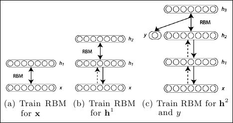
The training, in this case, is incremental; training layer by layer.
A network structure that recently achieves very good results at image recognition benchmarks is Convolutional Neural Network (CNN) or ConvNet. CNNs are a type of feedforward neural network that are structured in such a way that emulates behavior of the visual cortex, exploiting 2D structures of an input image, that is, patterns that exhibit spatially local correlation.
A CNN consists of a number of convolutional and subsampling layers, optionally followed by fully connected layers. An example is shown in the following image. The input layer reads all the pixels at an image and then we apply multiple filters. In the following image, four different filters are applied. Each filter is applied to the original image, for example, one pixel of a 6 x 6 filter is calculated as the weighted sum of a 6 x 6 square of input pixels and corresponding 6 x 6 weights. This effectively introduces filters similar to the standard image processing, such as smoothing, correlation, edge detection, and so on. The resulting image is called feature map. In the example in the image, we have four feature maps, one for each filter.
The next layer is the subsampling layer, which reduces the size of the input. Each feature map is subsampled typically with mean or max pooling over a contiguous region of 2 x 2 (up to 5 x 5 for large images). For example, if the feature map size is 16 x 16 and the subsampling region is 2 x 2, the reduced feature map size is 8 x 8, where 4 pixels (2 x 2 square) are combined into a single pixel by calculating max, min, mean, or some other functions:

The network may contain several consecutive convolution and subsampling layers, as shown in the preceding diagram. A particular feature map is connected to the next reduced/convoluted feature map, while feature maps at the same layer are not connected to each other.
After the last subsampling or convolutional layer, there is usually a fully connected layer, identical to the layers in a standard multilayer neural network, which represents the target data.
CNN is trained using a modified backpropagation algorithm that takes the subsampling layers into account and updates the convolutional filter weights based on all the values where this filter is applied.
This concludes our review of main neural network structures. In the following section, we'll move to the actual implementation.