
Among the first tools to master are the different feature analysis and dimensionality reduction techniques. As in supervised learning, the need for reducing dimensionality arises from numerous reasons similar to those discussed earlier for feature selection and reduction.
A smaller number of discriminating dimensions makes visualization of data and clusters much easier. In many applications, unsupervised dimensionality reduction techniques are used for compression, which can then be used for transmission or storage of data. This is particularly useful when the larger data has an overhead. Moreover, applying dimensionality reduction techniques can improve the scalability in terms of memory and computation speeds of many algorithms.
We will use similar notation to what was used in the chapter on supervised learning. The examples are in d dimensions and are represented as vector:
x = (x1,x2,…xd )T
The entire dataset containing n examples can be represented as an observation matrix:

The idea of dimensionality reduction is to find k ≤ d features either by transformation of the input features, projecting or combining them such that the lower dimension k captures or preserves interesting properties of the original dataset.
Linear dimensionality methods are some of the oldest statistical techniques to reduce features or transform the data into lower dimensions, preserving interesting discriminating properties.
Mathematically, with linear methods we are performing a transformation, such that a new data element is created using a linear transformation of the original data element:
s = Wx
Here, Wk × d is the linear transformation matrix. The variables s are also referred to as latent or hidden variables.
In this topic, we will discuss the two most practical and often-used methodologies. We will list some variants of these techniques so that the reader can use the tools to experiment with them. The main assumption here—which often forms the limitation—is the linear relationships between the transformations.
PCA is a widely-used technique for dimensionality reduction(References [1]). The original coordinate system is rotated to a new coordinate system that exploits the directions of maximum variance in the data, resulting in uncorrelated variables in a lower-dimensional subspace that were correlated in the original feature space. PCA is sensitive to the scaling of the features.
PCA is generally effective on numeric datasets. Many tools provide the categorical-to-continuous transformations for the nominal features, but this affects the performance. The number of principal components, or k, is also an input provided by the user.
PCA, in its most basic form, tries to find projections of data onto new axes, which are known as principal components. Principal components are projections that capture maximum variance directions from the original space. In simple words, PCA finds the first principal component through rotation of the original axes of the data in the direction of maximum variance. The technique finds the next principal component by again determining the next best axis, orthogonal to the first axis, by seeking the second highest variance and so on until most variances are captured. Generally, most tools give either a choice of number of principal components or the option to keep finding components until some percentage, for example, 99%, of variance in the original dataset is captured.
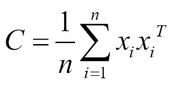
Mathematically, the objective of finding maximum variance can be written as

λ v = Cv is the eigendecomposition
This is equivalent to:
Here, W is the principal components and S is the new transformation of the input data. Generally, eigenvalue decomposition or singular value decomposition is used in the computation part.

Figure 1: Principal Component Analysis
- One of the advantages of PCA is that it is optimal in that it minimizes the reconstruction error of the data.
- PCA assumes normal distribution.
- The computation of variance-covariance matrix can become intensive for large datasets with high-dimensions. Alternatively, Singular Value Decomposition (SVD) can be used as it works iteratively and there is no need for an explicit covariance matrix.
- PCA has issues when there is noise in the data.
- PCA fails when the data lies in the complex manifold, a topic that we will discuss in the non-linear dimensionality reduction section.
- PCA assumes a correlation between the features and in the absence of those correlations, it is unable to do any transformations; instead, it simply ranks them.
- By transforming the original feature space into a new set of variables, PCA causes a loss in interpretability of the data.
- There are many other variants of PCA that are popular and overcome some of the biases and assumptions of PCA.
Independent Component Analysis (ICA) assumes that there are mixtures of non-Gaussians from the source and, using the generative technique, tries to find the decompositions of original data in the smaller mixtures or components (References [2]). The key difference between PCA and ICA is that PCA creates components that are uncorrelated, while ICA creates components that are independent.
Mathematically, it assumes ![]() as a mixture of independent sources ∈
as a mixture of independent sources ∈ ![]() , such that each data element y = [y
1
,y
2
,….y
k
]T and independence is implied by
, such that each data element y = [y
1
,y
2
,….y
k
]T and independence is implied by ![]() :
:
Probabilistic Principal Component Analysis (PPCA) is based on finding the components using mixture models and maximum likelihood formulations using Expectation Maximization (EM) (References [3]). It overcomes the issues of missing data and outlier impacts that PCA faces.
When data is separable by a large margin—even if it is high-dimensional data—one can randomly project the data down to a low-dimensional space without impacting separability and achieve good generalization with a relatively small amount of data. Random Projections use this technique and the details are described here (References [4]).
Random projections work with both numeric and categorical features, but categorical features are transformed into binary. Outputs are lower dimensional representations of the input data elements. The number of dimensions to project, k, is part of user-defined input.
This technique uses random projection matrices to project the input data into a lower dimensional space. The original data ![]() is transformed to the lower dimension space
is transformed to the lower dimension space ![]() where k << p using:
where k << p using:
Here columns in the k x d matrix R are i.i.d zero mean normal variables and are scaled to unit length. There are variants of how the random matrix R is constructed using probabilistic sampling. Computational complexity of RP is O(knd), which scales much better than PCA. In many practical datasets, it has been shown that RP gives results comparable to PCA and can scale to large dimensions and datasets.
There are many forms of MDS—classical, metric, and non-metric. The main idea of MDS is to preserve the pairwise similarity/distance values. It generally involves transforming the high dimensional data into two or three dimensions (References [5]).
MDS can work with both numeric and categorical data based on the user-selected distance function. The number of dimensions to transform to, k, is a user-defined input.
Given n data elements, an n x n affinity or distance matrix is computed. There are choices of using distances such as Euclidean, Mahalanobis, or similarity concepts such as cosine similarity, Jaccard coefficients, and so on. MDS in its very basic form tries to find a mapping of the distance matrix in a lower dimensional space where the Euclidean distance between the transformed points is similar to the affinity matrix.
Mathematically:

Here ![]() input space and
input space and ![]() mapped space.
mapped space.
If the input affinity space is transformed using kernels then the MDS becomes a non-linear method for dimensionality reduction. Classical MDS is equivalent to PCA when the distances between the points in input space is Euclidean distance.
- The key disadvantage is the subjective choice of the lower dimension needed to interpret the high dimensional data, normally restricted to two or three for humans. Some data may not map effectively in this lower dimensional space.
- The advantage is you can perform linear and non-linear mapping to the lowest dimensions using the framework.
In general, nonlinear dimensionality reduction involves either performing nonlinear transformations to the computations in linear methods such as KPCA or finding nonlinear relationships in the lower dimension as in manifold learning. In some domains and datasets, the structure of the data in lower dimensions is nonlinear—and that is where techniques such as KPCA are effective—while in some domains the data does not unfold in lower dimensions and you need manifold learning.
Kernel PCA uses the Kernel trick described in Chapter 2, Practical Approach to Real-World Supervised Learning, with the PCA algorithm for transforming the data in a high-dimensional space to find effective mapping (References [6]).
Similar to PCA with addition of choice of kernel and kernel parameters. For example, if Radial Basis Function (RBF) or Gaussian Kernel is chosen, then the kernel, along with the gamma parameter, becomes user-selected values.
In the same way as Support Vector Machines (SVM) was discussed in the previous chapter, KPCA transforms the input space to high dimensional feature space using the "kernel trick". The entire PCA machinery of finding maximum variance is then carried out in the transformed space.
As in PCA:
Instead of linear covariance matrix, a nonlinear transformation is applied to the input space using kernel methods by constructing the N x N matrix, in place of doing the actual transformations using ϕ (x).
k(x,y) = (( ϕ (x), ϕ (y)) = ϕ (x) T ϕ (y)
Since the kernel transformation doesn't actually transform the features into explicit feature space, the principal components found can be interpreted as projections of data onto the components. In the following figure, a binary nonlinear dataset, generated using the scikit-learn example on circles (References [27]), demonstrates the linear separation after KPCA using the RBF kernel and returning to almost similar input space by the inverse transform:

Figure 2: KPCA on Circle Dataset and Inverse Transform.
- KPCA overcomes the nonlinear mapping presented by PCA.
- KPCA has similar issues with outlier, noisy, and missing values to standard PCA. There are robust methods and variations to overcome this.
- KPCA has scalability issues in space due to an increase in the kernel matrix, which can become a bottleneck in large datasets with high dimensions. SVD can be used in these situations, as an alternative.
When high dimensional data is embedded in lower dimensions that are nonlinear, but have complex structure, manifold learning is very effective.
Manifold learning algorithms require two user-provided parameters: k, representing the number of neighbors for the initial search, and n, the number of manifold coordinates.
As seen in the following figure, the three-dimensional S-Curve, plotted using the scikit-learn utility (References [27]), is represented in 2D PCA and in 2D manifold using LLE. It is interesting to observe how the blue, green, and red dots are mixed up in the PCA representation while the manifold learning representation using LLE cleanly separates the colors. It can also be observed that the rank ordering of Euclidean distances is not maintained in the manifold representation:

Figure 3: Data representation after PCA and manifold learning
To preserve the structure, the geodesic distance is preserved instead of the Euclidean distance. The general approach is to build a graph structure such as an adjacency matrix, and then compute geodesic distance using different assumptions. In the Isomap Algorithm, the global pairwise distances are preserved (References [7]). In the Local Linear Embedding (LLE) Algorithm, the mapping is done to take care of local neighborhood, that is, nearby points map to nearby points in the transformation (References [9]). Laplacian Eigenmaps is similar to LLE, except it tries to maintain the "locality" instead of "local linearity" in LLE by using graph Laplacian (References [8]).