
The case study in this chapter consists of several experiments that illustrate different methods of stream-based machine learning. A well-studied dataset was chosen as the stream data source and supervised tree based methods such as Naïve Bayes, Hoeffding Tree, as well as ensemble methods, were used. Among unsupervised methods, clustering algorithms used include k-Means, DBSCAN, CluStream, and CluTree. Outlier detection techniques include MCOD and SimpleCOD, among others. We also show results from classification experiments that demonstrate handling concept drift. The ADWIN algorithm for calculating statistics in a sliding window, as described earlier in this chapter, is employed in several algorithms used in the classification experiments.
One of the most popular and arguably the most comprehensive Java-based frameworks for data stream mining is the open source Massive Online Analysis (MOA) software created by the University of Waikato. The framework is a collection of stream classification, clustering, and outlier detection algorithms and has support for change detection and concept drift. It also includes data generators and several evaluation tools. The framework can be extended with new stream data generators, algorithms, and evaluators. In this case study, we employ several stream data learning methods using a file-based data stream.
As shown in the series of screenshots from the MOA tool shown in Figure 4 and Figure 5, the top-level menu lets you choose the type of learning to be done. For the classification experiments, for example, configuration of the tools consists of selecting the task to run (selected to be prequential evaluation here), and then configuring which learner and evaluator we want to use, and finally, the source of the data stream. A window width parameter shown in the Configure Task dialog can affect the accuracy of the model chosen, as we will see in the experiment results. Other than choosing different values for the window width, all base learner parameters were left as default values. Once the task is configured it is run by clicking the Run button:

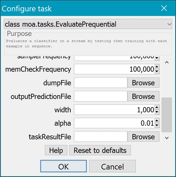
Figure 4. MOA graphical interface for configuring prequential evaluation for classification which includes setting the window width


Figure 5. MOA graphical interface for prequential classification task. Within the Configure task, you must choose a learner, locate the data stream (details not shown), and select an evaluator
After the task has completed running, model evaluation results can be exported to a CSV file.
The problem for this case study is to continuously learn from a stream of electricity market data and predict the direction of movement of the market price. We compare the accuracy and average cost of different classification methods including concept drift as well as the performance of clustering and outlier detection.
The dataset used in this case study can be used to illustrate classical batch-based supervised and unsupervised learning techniques. However, here we treat it as a stream-based data source to show how we can employ the techniques described in this chapter to perform classification, clustering, and outlier detection tasks using the MOA framework. Within this context, we demonstrate how incremental learning can be achieved under assumptions of a stationary as well as an evolving data stream exhibiting concept drift.
The dataset is known as the Electricity or ELEC dataset, which was collected by the New South Wales Electricity Market. The prices in this market are variable, and are adjusted every 5 minutes based on supply and demand. This dataset consists of 45,312 such data points obtained every half-hour between May 1996 and December 1998. The target is an indication of the movement of the price, whether up or down, relative to the 24-hour moving average.
Note
The data file is a publicly available file in the ARRF format at http://downloads.sourceforge.net/project/moa-datastream/Datasets/Classification/elecNormNew.arff.zip?r=http%3A%2F%2Fmoa.cms.waikato.ac.nz%2Fdatasets%2F&ts=1483128450&use_mirror=cytranet.
In the experiments conducted here, no data sampling is done; each example in the dataset is processed individually and no example is excluded. All numeric data elements have been normalized to a value between 0 and 1.
The ELEC dataset has 45,312 records with nine features, including the target class. The features class and day are nominal (categorical), all others are numeric (continuous). The features are listed in Table 1 and Table 2 and give descriptive statistics for the ELEC dataset:
|
Name |
Data Type |
Description |
|---|---|---|
|
class |
nominal |
UP, DOWN—direction of price movement relative to 24-hour moving average |
|
date |
continuous |
Date price recorded |
|
day |
nominal |
Day of the week (1-7) |
|
period |
continuous | |
|
nswprice |
continuous |
Electricity price in NSW |
|
nswdemand |
continuous |
Electricity demand in NSW |
|
vicprice |
continuous |
Electricity price in Victoria |
|
vicdemand |
continuous |
Electricity demand in Victoria |
|
transfer |
integer |
Table 1. ELEC dataset features
|
count |
mean |
std |
25% |
50% |
75% | |
|---|---|---|---|---|---|---|
|
date |
45312 |
0.49908 |
0.340308 |
0.031934 |
0.456329 |
0.880547 |
|
period |
45312 |
0.5 |
0.294756 |
0.25 |
0.5 |
0.75 |
|
nswprice |
45312 |
0.057868 |
0.039991 |
0.035127 |
0.048652 |
0.074336 |
|
nswdemand |
45312 |
0.425418 |
0.163323 |
0.309134 |
0.443693 |
0.536001 |
|
vicprice |
45312 |
0.003467 |
0.010213 |
0.002277 |
0.003467 |
0.003467 |
|
vicdemand |
45312 |
0.422915 |
0.120965 |
0.372346 |
0.422915 |
0.469252 |
|
transfer |
45312 |
0.500526 |
0.153373 |
0.414912 |
0.414912 |
0.605702 |
Table 2. Descriptive statistics of ELEC dataset features
The feature reduction step is omitted here as it is in most stream-based learning.
The experiments are divided into classification, concept drift, clustering, and outlier detection. Details of the learning process for each set of experiments and the results of the experiments are given here.
For this set of experiments, a choice of linear, non-linear, and ensemble learners were chosen in order to illustrate the behavior of a variety of classifiers. Stochastic Gradient Descent (SGD), which uses a linear SVM, and Naïve Bayes are the linear classifiers, while Lazy k-NN is the non-linear classifier. For ensemble learning, we use two meta-learners, Leveraging Bagging (LB) and OxaBag, with different linear and non-linear base learners such as SGD, Naïve Bayes, and Hoeffding Trees. The algorithm used in OxaBag is described in the section on ensemble algorithms. In LB, the weight factor used for resampling is variable (the default value of 6 is used here) whereas the weight in OxaBag is fixed at 1.
Prequential evaluation is chosen for all the classification methods, so each example is first tested against the prediction with the existing model, and then used for training the model. This requires the selection of a window width, and the performance of the various models for different values of the window width are listed in Table 3. Widths of 100, 500, 1,000, and 5,000 elements were used:
|
Algorithm |
Window width |
Evaluation time (CPU seconds) |
Model cost (RAM-Hours) |
Classifications correct (percent) |
Kappa Statistic (percent) |
|---|---|---|---|---|---|
|
SGD |
100 |
0.5781 |
3.76E-10 |
67 |
0 |
|
SGD |
500 |
0.5781 |
3.76E-10 |
55.6 |
0 |
|
SGD |
1000 |
0.5469 |
3.55E-10 |
53.3 |
0 |
|
SGD |
5000 |
0.5469 |
3.55E-10 |
53.78 |
0 |
|
NaiveBayes |
100 |
0.7656 |
8.78E-10 |
86 |
65.7030 |
|
NaiveBayes |
500 |
0.6094 |
8.00E-10 |
82.2 |
62.6778 |
|
NaiveBayes |
1000 |
0.6719 |
7.77E-10 |
75.3 |
48.8583 |
|
NaiveBayes |
5000 |
0.6406 |
7.35E-10 |
77.84 |
54.1966 |
|
kNN |
100 |
34.6406 |
4.66E-06 |
74 |
36.3057 |
|
kNN |
500 |
34.5469 |
4.65E-06 |
79.8 |
59.1424 |
|
kNN |
1000 |
35.8750 |
4.83E-06 |
82.5 |
64.8049 |
|
kNN |
5000 |
35.0312 |
4.71E-06 |
80.32 |
60.4594 |
|
LB-kNN |
100 |
637.8125 |
2.88E-04 |
74 |
36.3057 |
|
LB-kNN |
500 |
638.9687 |
2.89E-04 |
79.8 |
59.1424 |
|
LB-kNN |
1000 |
655.8125 |
2.96E-04 |
82.4 |
64.5802 |
|
LB-kNN |
5000 |
667.6094 |
3.02E-04 |
80.66 |
61.0965 |
|
LB-HoeffdingTree |
100 |
13.6875 |
2.98E-06 |
91 |
79.1667 |
|
LB-HoeffdingTree |
500 |
13.5781 |
2.96E-06 |
93 |
85.8925 |
|
LB-HoeffdingTree |
1000 |
12.5625 |
2.74E-06 |
92.1 |
84.1665 |
|
LB-HoeffdingTree |
5000 |
12.7656 |
2.78E-06 |
90.74 |
81.3184 |
Table 3. Classifier performance for different window sizes
For the algorithms in Table 4, the performance was the same for each value of the window width used:
|
Algorithm |
Evaluation time (CPU seconds) |
Model cost (RAM-Hours) |
Classifications correct (percent) |
Kappa Statistic (percent) |
|---|---|---|---|---|
|
HoeffdingTree |
1.1562 |
3.85E-08 |
79.1953 |
57.2266 |
|
HoeffdingAdaptiveTree |
2.0469 |
2.84E-09 |
83.3863 |
65.5569 |
|
OzaBag-NaiveBayes |
2.01562 |
1.57E-08 |
73.4794 |
42.7636 |
|
OzaBagAdwin-HoeffdingTree |
5.7812 |
2.26E-07 |
84.3485 |
67.5221 |
|
LB-SGD |
2 |
1.67E-08 |
57.6977 |
3.0887 |
|
LB-NaiveBayes |
3.5937 |
3.99E-08 |
78.8753 |
55.7639 |
Table 4. Performance of classifiers (same for all window widths used)
In this experiment, we continue using EvaluatePrequential when configuring the classification task. This time we select the DriftDetectionMethodClassifier as the learner and DDM as the drift detection method. This demonstrates adapting to an evolving data stream. Base learners used and the results obtained are shown in Table 5:
|
Algorithm |
Evaluation time (CPU seconds) |
Model cost (RAM-Hours) |
Classifications correct (percent) |
Kappa Statistic (percent) |
Change detected |
|---|---|---|---|---|---|
|
SGD |
0.307368829 |
1.61E-09 |
53.3 |
0 |
132 |
|
Naïve-Bayes |
0.298290727 |
1.58E-09 |
86.6 |
73.03986 |
143 |
|
Lazy-kNN |
10.34161893 |
1.74E-06 |
87.4 |
74.8498 |
12 |
|
HoeffdingTree |
0.472981754 |
5.49E-09 |
86.2 |
72.19816 |
169 |
|
HoeffdingAdaptiveTree |
0.598665043 |
7.19E-09 |
84 |
67.80878 |
155 |
|
LB-SGD |
0.912737325 |
2.33E-08 |
53.3 |
0 |
132 |
|
LB-NaiveBayes |
1.990137758 |
3.61E-08 |
85.7 |
71.24056 |
205 |
|
OzaBag-NaiveBayes |
1.342189725 |
2.29E-08 |
77.4 |
54.017 |
211 |
|
LB-kNN |
173.3624715 |
1.14E-04 |
87.5 |
75.03296 |
4 |
|
LB-HoeffdingTree |
5.660440101 |
1.61E-06 |
91.3 |
82.56317 |
59 |
|
OzaBag-HoeffdingTree |
4.306455545 |
3.48E-07 |
85.4 |
70.60209 |
125 |
Table 5. Performance of classifiers with concept drift detection
Almost all of the clustering algorithms implemented in the MOA tool were used in this experiment. Both extrinsic and intrinsic evaluation results were collected and are tabulated in Table 6. CMM, homogeneity, and completeness were defined earlier in this chapter. We have encountered Purity and Silhouette coefficients before, from the discussion in Chapter 3, Unsupervised Machine Learning Techniques. SSQ is the sum of squared distances of instances from their respective cluster centers; the lower the value of SSQ, the better. The use of micro-clustering is indicated by m = 1 in the table. How often the macro-clusters are calculated is determined by the selected time horizon h, in instances:
|
Algorithm |
CMM |
Homogeneity |
Completeness |
Purity |
SSQ |
Silhouette Coefficient |
|---|---|---|---|---|---|---|
|
Clustream With k-Means (h = 5000; k = 2; m = 1) |
0.7168 |
-1.0000 |
0.1737 |
0.9504 |
9.1975 |
0.5687 |
|
Clustream With k-Means (h = 1000; k = 5) |
0.5391 |
-1.0000 |
0.8377 |
0.7238 |
283.6543 |
0.8264 |
|
Clustream (h = 1000; m = 1) |
0.6241 |
-1.0000 |
0.4363 |
0.9932 |
7.2734 |
0.4936 |
|
Denstream With DBSCAN (h = 1000) |
0.4455 |
-1.0000 |
0.7586 |
0.9167 |
428.7604 |
0.6682 |
|
ClusTree (h = 5000; m = 1) |
0.7984 |
0.4874 |
-0.4815 |
0.9489 |
11.7789 |
0.6879 |
|
ClusTree (h = 1000; m = 1) |
0.7090 |
-1.0000 |
0.3979 |
0.9072 |
13.4190 |
0.5385 |
|
AbstractC |
1.0000 |
1.0000 |
-8.1354 |
1.0000 |
0.0000 |
0.0000 |
|
MCOD (w = 1000) |
1.0000 |
1.0000 |
-8.1354 |
1.0000 |
0.0000 |
0.0000 |
In the final set of experiments, five outlier detection algorithms were used to process the ELEC dataset. Results are given in Table 7:
|
Algorithm |
Nodes always inlier |
Nodes always outlier |
Nodes both inlier and outlier |
|---|---|---|---|
|
MCOD |
42449 (93.7%) |
302 (0.7%) |
2561 (5.7%) |
|
ApproxSTORM |
41080 (90.7%) |
358 (0.8%) |
3874 (8.5%) |
|
SimpleCOD |
42449 (93.7%) |
302 (0.7%) |
2561 (5.7%) |
|
AbstractC |
42449 (93.7%) |
302 (0.7%) |
2561 (5.7%) |
|
ExactSTORM |
42449 (93.7%) |
302 (0.7%) |
2561 (5.7%) |
Table 7. Evaluation of outlier detection
The following plots (Figure 6) show results for three pairs of features after running algorithm Abstract-C on the entire dataset. In each of the plots, it is easy to see the outliers identified by the circles surrounding the data points. Although it is difficult to visualize the outliers spatially in multiple dimensions simultaneously, the set bi-variate plots give some indication of the result of outlier detection methods applied in a stream-based setting:


Figure 6. Outlier detection using Abstract-C, for three pairs of features, after processing all 45,300 instances
The image in Figure 7 shows a screenshot from MOA when two algorithms, Angiulli.ExactSTORM and Angiulli.ApproxSTORM, were run simultaneously; a bivariate scatter-plot for each algorithm is shown side-by-side, accompanied by a comparison of the per-object processing time:

Figure 7. Visualization of outlier detection in MOA
Based on the evaluation of the learned models from the classification, clustering, and outlier detection experiments, analysis reveals several interesting observations.
Classification experiments:
- Performance improves from linear to non-linear algorithms in quite a significant way as shown in Table 3. Linear SGD has the best performance using an accuracy metric of 67%, while KNN and Hoeffding Tree show 82.4 to 93%. This clearly shows that the problem is non-linear and using a non-linear algorithm will give better performance.
- K-NNs give good performance but come at the cost of evaluation time, as shown in Table 3. Evaluation time as well as memory are significantly higher—about two orders of magnitude—than the linear methods. When the model has to perform in tighter evaluation cycles, extreme caution in choosing algorithms such as KNNs must be observed.
- Hoeffding Trees gives the best classification rate and Kappa statistic. The evaluation time is also not as high as KNNs but is still in the order of seconds, which may or may not be acceptable in many real-time stream-based applications.
- The evaluation time of Naive Bayes is the lowest—though not much different from SGD—and with the right choice of window width can give performance second only to Hoeffding Trees. For example, at width 100, we have a classification rate of 86 with Naïve Bayes, which is next best to 93 of Hoeffding Trees but compared to over 13 seconds, Naïve Bayes takes only 0.76 seconds, as shown in Table 3.
- Keeping the window width constant, there is a clear pattern of improvement from linear (SGD, Naïve Bayes) to non-linear (Hoeffding Trees) to ensemble based (OzaBag, Adwin, Hoeffding Tree) shown in Table 4. This clearly shows that in theory, the choice of ensembles can help reduce the errors but comes at the cost of foregoing interpretability in the models.
- Table 5, when compared to Table 3 and Table 4, shows why having drift protection and learning with automated drift detection increases robustness. Ensemble-based learning of OzaBag-NaiveBayes, OzaBag-HoeffdingTrees, and OzaBag-HoeffdingAdaptiveTree all show improvements over the non- drift protected runs as an example.
Clustering experiments:
- From the first two models in Table 6, we see that k-Means, with a horizon of 5,000 instances and k of 2, exhibits higher purity, higher CMM, and lower SSQ compared to the model with a smaller horizon and k of 5. In the complete set of results (available on this book's website, see link below), one can see that the effect of the larger horizon is the predominant factor responsible for the differences.
- In the clustering models using micro-clustering, the SSQ is typically significantly smaller than when no micro-clustering is used. This is understandable, as there are far more clusters and fewer instances per cluster, and SSQ is measured with respect to the cluster center.
- DBSCAN was found to be insensitive to micro-clustering, and size of the horizon. Compared to all other models, it ranks high on both intrinsic (Silhouette coefficient) as well as extrinsic measures (Completeness, Purity).
- The two ClusTree models have among the best CMM and Purity scores, with low SSQ due to micro-clusters.
- The final two outlier-based clustering algorithms have perfect CMM and Purity scores. The metrics are not significantly affected by the window size (although this impacts the evaluation time), or the value of k, the neighbor count threshold.
Outlier detection experiments:
- All the techniques in this set of experiments performed equally well, with the exception of ApproxSTORM, which is to be expected considering the reduced window used in this method compared to the exact version.
- The ratio of instances, always inlier versus those always outlier, is close to 140 for the majority of the models. Whether this implies adequate discriminatory power for a given dataset depends on the goals of the real-time learning problem.
Note
All MOA configuration files and results from the experiments are available at: https://github.com/mjmlbook/mastering-java-machine-learning/Chapter5.