
So far, we have covered directed acyclic graphs in the area of probabilistic graph models, including every aspect of representation, inference, and learning. When the graphs are undirected, they are known as Markov networks (MN) or Markov random field (MRF). We will discuss some aspects of Markov networks in this section covering areas of representation, inference, and learning, as before. Markov networks or MRF are very popular in various areas of computer vision such as segmentation, de-noising, stereo, recognition, and so on. For further reading, see (References [10]).
Even though a Markov network, like Bayesian networks, has undirected edges, it still has local interactions and distributions. We will first discuss the concept of parameterization, which is a way to capture these interactions, and then the independencies in MN.
The affinities between the variables in MN are captured through three alternative parameterization techniques discussed in the following sections.
The probability distribution function is said to be in Gibb's distribution or parameterized by Gibb's distribution if

Z is called the partitioning function defined as:

Note that interaction between variables are captured by factors ![]() and are not the marginal probabilities, but contribute to the joint probability. The factors that parameterize a Markov network are called clique potentials. By choosing factors over maximal cliques in the graph, the number of parameters are reduced substantially.
and are not the marginal probabilities, but contribute to the joint probability. The factors that parameterize a Markov network are called clique potentials. By choosing factors over maximal cliques in the graph, the number of parameters are reduced substantially.
Graph structure of Markov network does not reveal properties such as whether the factors involve maximal cliques or their subsets when using Gibbs parameterization. Factor graphs discussed in the section of inferencing in Bayesian networks have a step to recognize maximal cliques and thus can capture these parameterizations. Please refer to the section on factor graphs in BN.
Another form of parameterization is to use the energy model representation from statistical physics.
The potential is represented as a set of features and a potential table is generally represented by features with weights associated with them.
If D is a set of variables, ![]() is a factor then:
is a factor then:

Thus, as the energy increases, the probability decreases and vice versa. The logarithmic cell frequencies captured in ![]() are known as log-linear in statistical physics. The joint probability can be represented as:
are known as log-linear in statistical physics. The joint probability can be represented as:

![]() is the feature function defined over the variables in Di.
is the feature function defined over the variables in Di.
Like Bayesian networks, Markov networks also encode a set of independence assumptions governing the flow of influence in undirected graphs.
A set of nodes Z separates sets of nodes X and Y, if there is no active path between any node in X ? X and Y ? Y given Z. Independence in graph G is:

Two nodes, X and Y, are independent given all other nodes if there is no direct edge between them. This property is of local independence and is weakest of all:

A node is independent of all other nodes in the graph, given its Markov blanket, which is an important concept in Markov networks:

Here U = markov blanket of X.
Figure 15 shows a Markov blanket for variable X as its parents, children, and children's parents:

Figure 15. Markov blanket for Node X - its Parents, Children, and Children's Parents.
Inference in MNs is similarly #P-complete problem and hence similar approximations or heuristics get applied. Most exact and approximate inferencing techniques, such as variable elimination method, junction tree method, belief propagation method, and so on, which were discussed in Bayes network, are directly applicable to Markov networks. The marginals and conditionals remain similar and computed over the potential functions over the cliques as


Markov blankets simplify some of the computations.
Learning the parameters in Markov networks is complex and computationally expensive due to the entanglement of all the parameters in the partitioning function. The advantageous step of decomposing the computations into local distributions cannot be done because of the partitioning function needing the factor coupling of all the variables in the network.
Maximum likelihood estimation in MN does not have a closed–form solution and hence incremental techniques such as gradient descent are used for optimizing over the entire parameter space. The optimization function can be shown to be a concave function, thus ensuring a global optimum, but each step of the iterations in gradient descent requires inferencing over the entire network, making it computationally expensive and sometimes intractable.
Bayesian parameter estimation requires integration over the entire space of parameters, which again has no closed-form solution and is even harder. Thus, most often, approximate learning methods such as Markov Chain Monte Carlo (MCMC) are used for MNs.
Structure learning in the MNs is similar or even harder than parameter learning and has been shown to be NP-hard. In the constraint-based approach, for a given dataset, conditional independence between the variables is tested. In MNs, each pair of variables is tested for conditional independence using mutual information between the pair. Then, based on a threshold, an edge is either considered to be existing between the pair or not. One disadvantage of this is it requires extremely large numbers of samples to refute any noise present in the data. Complexity of the network due to occurrence of pairwise edges is another limitation.
In search and score-based learning, the goal is similar to BNs, where search is done for structures and scoring—based on various techniques—is computed to help and adjust the search. In the case of MNs, we use features described in the log-linear models rather than the potentials. The weighting of the features is considered during optimization and scoring.
Conditional random fields (CRFs) are a specialized form of Markov network where the hidden and observables are mostly modeled for labeled sequence prediction problems (References [16]). Sequence prediction problems manifest in many text mining areas such as next word/letter predictions, Part of speech (POS) tagging, and so on, and in bioinformatics domain for DNA or protein sequence predictions.
The idea behind CRFs is the conditional distribution of sequence is modeled as feature functions and the labeled data is used to learn using optimization the empirical distribution, as shown in the following figure.
The conditional distribution is expressed as follows where Z(x) is the normalizing constant. Maximum likelihood is used for parameter estimation for ? and is generally a convex function in log-linear obtained through iterative optimization methods such as gradient descent.
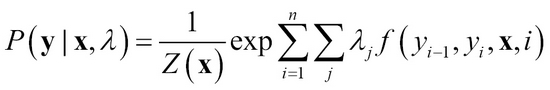

Figure 16: Conditional random fields mapped to the area of sequence prediction in the POS tagging domain.