
In this case study, we use the CoverType dataset to demonstrate classification and clustering algorithms from H2O, Apache Spark MLlib, and SAMOA Machine Learning libraries in Java.
The CoverType dataset available from the UCI machine learning repository (https://archive.ics.uci.edu/ml/datasets/Covertype) contains unscaled cartographic data for 581,012 cells of forest land 30 x 30 m2 in dimension, accompanied by actual forest cover type labels. In the experiments conducted here, we use the normalized version of the data. Including one-hot encoding of two categorical types, there are a total of 54 attributes in each row.
First, we treat the problem as one of classification using the labels included in the dataset and perform several supervised learning experiments. With the models generated, we make predictions about the forest cover type of an unseen held out test dataset. For the clustering experiments that follow, we ignore the data labels, determine the number of clusters to use, and then report the corresponding cost using various algorithms implemented in H2O and Spark MLLib.
This dataset was collected using cartographic measurements only and no remote sensing. It was derived from data originally collected by the US Forest Service (USFS) and the US Geological Survey (USGS).
Train and test data—The dataset was split into two sets in the ratio 20% for testing and 80% for training.
The categorical Soil Type designation was represented by 40 binary variable attributes. A value of 1 indicates the presence of a soil type in the observation; a 0 indicates its absence.
The wilderness area designation is likewise a categorical attribute with four binary columns, with 1 indicating presence and 0 absence.
All continuous value attributes have been normalized prior to use.
In the first set of experiments in this case study, we used the H2O framework.
Though H2O doesn't have explicit feature selection algorithms, many learners such as GLM, random forest, GBT, and so on, give feature importance metrics based on training/validation of the models. In our analysis, we have used GLM for feature selection, as shown in Figure 16. It is interesting that the feature Elevation emerges as the most discriminating feature along with some categorical features that are converted into numeric/binary such as Soil_Type2, Soil_Type4, and so on. Many of the soil type categorical features have no relevance and can be dropped from the modeling perspective.
Learning algorithms included in this set of experiments were: Generalized Linear Models (GLM), Gradient Boosting Machine (GBM), Random Forest (RF), Naïve Bayes (NB), and Deep Learning (DL). The deep learning model supported by H2O is the multi-layered perceptron (MLP).

Figure 16: Feature selection using GLM
The results using all the features are shown in the table:
|
Algorithm |
Parameters |
AUC |
Max Accuracy |
Max F1 |
Max Precision |
Max Recall |
Max Specificity |
|---|---|---|---|---|---|---|---|
|
GLM |
Default |
0.84 |
0.79 |
0.84 |
0.98 |
1.0(1) |
0.99 |
|
GBM |
Default |
0.86 |
0.82 |
0.86 |
1.0(1) |
1.0(1) |
1.0(1) |
|
Random Forest (RF) |
Default |
0.88(1) |
0.83(1) |
0.87(1) |
0.97 |
1.0(1) |
0.99 |
|
Naïve Bayes (NB) |
Laplace=50 |
0.66 |
0.72 |
0.81 |
0.68 |
1.0(1) |
0.33 |
|
Deep Learning (DL) |
Rect,300, 300,Dropout |
0. |
0.78 |
0.83 |
0.88 |
1.0(1) |
0.99 |
|
Deep Learning (DL) |
300, 300,MaxDropout |
0.82 |
0.8 |
0.84 |
1.0(1) |
1.0(1) |
1.0(1) |
The results after removing features not scoring well in feature relevance were:
|
Algorithm |
Parameters |
AUC |
Max Accuracy |
Max F1 |
Max Precision |
Max Recall |
Max Specificity |
|---|---|---|---|---|---|---|---|
|
GLM |
Default |
0.84 |
0.80 |
0.85 |
1.0 |
1.0 |
1.0 |
|
GBM |
Default |
0.85 |
0.82 |
0.86 |
1.0 |
1.0 |
1.0 |
|
Random Forest (RF) |
Default |
0.88 |
0.83 |
0.87 |
1.0 |
1.0 |
1.0 |
|
Naïve Bayes (NB) |
Laplace=50 |
0.76 |
0.74 |
0.81 |
0.89 |
1.0 |
0.95 |
|
Deep Learning (DL) |
300,300, RectDropout |
0.81 |
0.79 |
0.84 |
1.0 |
1.0 |
1.0 |
|
Deep Learning (DL) |
300, 300, MaxDropout |
0.85 |
0.80 |
0.84 |
0.89 |
0.90 |
1.0 |
Table 1: Model evaluation results with all features included
The main observations from an analysis of the results obtained are quite instructive and are presented here.
- The feature relevance analysis shows how the Elevation feature is a highly discriminating feature, whereas many categorical attributes converted to binary features, such as SoilType_10, and so on, have near-zero to no relevance.
- The results for experiments with all features included, shown in Table 1, clearly indicate that the non-linear ensemble technique Random Forest is the best algorithm as shown by the majority of the evaluation metrics including accuracy, F1, AUC, and recall.
- Table 1 also highlights the fact that whereas the faster, linear Naive Bayes algorithm may not be best-suited, GLM, which also falls in the category of linear algorithms, demonstrates much better performance—this points to some inter-dependence among features!
- As we saw in Chapter 7, Deep Learning, algorithms used in deep learning typically need a lot of tuning; however, even with a few small tuning changes, the results from DL are comparable to Random Forest, especially with MaxDropout.
- Table 2 shows the results of all the algorithms after removing low-relevance features from the training set. It can be seen that Naive Bayes—which has the most impact due to multiplication of probabilities based on the assumption of independence between features—gets the most benefit and highest uplift in performance. Most of the other algorithms such as Random Forest have inbuilt feature selection as we discussed in Chapter 2, Practical Approach to Real-World Supervised Learning, and as a result removing the unimportant features has little or no effect on their performance.
Apache Spark, started in 2009 at AMPLab at UC Berkley, was donated to Apache Software Foundation in 2013 under Apache License 2.0. The core idea of Spark was to build a cluster computing framework that would overcome the issues of Hadoop, especially for iterative and in-memory computations.
The Spark stack as shown in Figure 17 can use any kind of data stores such as HDFS, SQL, NoSQL, or local filesystems. It can be deployed on Hadoop, Mesos, or even standalone.
The most important component of Spark is the Spark Core, which provides a framework to handle and manipulate the data in a high-throughput, fault-tolerant, and scalable manner.
Built on top of Spark core are various libraries each meant for various functionalities needed in processing data and doing analytics in the Big Data world. Spark SQL gives us a language for performing data manipulation in Big Data stores using a querying language very much like SQL, the lingua franca of databases. Spark GraphX provides APIs to perform graph-related manipulations and graph-based algorithms on Big Data. Spark Streaming provides APIs to handle real-time operations needed in stream processing ranging from data manipulations to queries on the streams.
Spark-MLlib is the Machine Learning library that has an extensive set of Machine Learning algorithms to perform supervised and unsupervised tasks from feature selection to modeling. Spark has various language bindings such as Java, R, Scala, and Python. MLlib has a clear advantage running on top of the Spark engine, especially because of caching data in memory across multiple nodes and running MapReduce jobs, thus improving performance as compared to Mahout and other large-scale Machine Learning engines by a significant factor. MLlib also has other advantages such as fault tolerance and scalability without explicitly managing it in the Machine Learning algorithms.

Figure 17: Apache Spark high level architecture
The Spark core has the following components:
- Resilient Distributed Datasets (RDD): RDDs are the basic immutable collection of objects that Spark Core knows how to partition and distribute across the cluster for performing tasks. RDDs are composed of "partitions", dependent on parent RDDs and metadata about data placement.
- Two distinct operations are performed on RDDs:
- Transformations: Operations that are lazily evaluated and transform one RDD into another. Lazy evaluation defers evaluation as long as possible, which makes some resource optimizations possible.
- Action: The actual operation that triggers transformations and returns output values
- Lineage graph: The pipeline or flow of data describing the computation for a particular task, including different RDDs created in transformations and actions is known as the lineage graph of the task. The lineage graph plays a key role in fault tolerance.

Figure 18: Apache Spark lineage graph
Spark is agnostic to the cluster management and can work with several implementations—including YARN and Mesos—for managing the nodes, distributing the work, and communications. The distribution of tasks in Transformations and Actions across the cluster is done by the scheduler, starting from the driver node where the Spark context is created, to the many worker nodes as shown in Figure 19. When running with YARN, Spark gives the user the choice of the number of executors, heap, and core allocation per JVM at the node level.

Figure 19: Apace Spark cluster deployment and task distribution
Spark MLlib has a comprehensive Machine Learning toolkit, offering more algorithms than H2O at the time of writing, as shown in Figure 20:

Figure 20: Apache Spark MLlib machine learning algorithms
Many extensions have been written for Spark, including Spark MLlib, and the user community continues to contribute more packages. You can download third-party packages or register your own at https://spark-packages.org/.
Spark MLlib provides APIs for other languages in addition to Java, including Scala, Python, and R. When a SparkContext is created, it launches a monitoring and instrumentation web console at port 4040, which lets us see key information about the runtime, including scheduled tasks and their progress, RDD sizes and memory use, and so on. There are also external profiling tools available for use.
The business problem we tackled here is the same as the one described earlier for experiments using H2O. We employed five learning algorithms using MLlib, in all. The first was k-Means with all features using a k value determined from computing the cost—specifically, the Sum of Squared Errors (SSE)—over a large number of values of k and selecting the "elbow" of the curve. Determining the optimal value of k is typically not an easy task; often, evaluation measures such as silhouette are compared in order to pick the best k. Even though we know the number of classes in the dataset is 7, it is instructive to see where experiments like this lead if we pretend we did not have labeled data. The optimal k found using the elbow method was 27. In the real world, business decisions may often guide the selection of k.
In the following listings, we show how to use different models from the MLlib suite to do cluster analysis and classification. The code is based on examples available in the MLlib API Guide (https://spark.apache.org/docs/latest/mllib-guide.html). We use the normalized UCI CoverType dataset in CSV format. Note that it is more natural to use spark.sql.Dataset with the newer spark.ml package, whereas the spark.mllib package works more closely with JavaRDD. This provides an abstraction over RDDs and allows for optimization of the transformations beneath the covers. In the case of most unsupervised learning algorithms, this means the data must be transformed such that the dataset to be used for training and testing should have a column called features by default that contains all the features of an observation as a vector. A VectorAssembler object can be used for this transformation. A glimpse into the use of ML pipelines, which is a way to chain tasks together, is given in the source code for training a Random Forest classifier.
The following code fragment for the k-Means experiment uses the algorithm from the org.apache.spark.ml.clustering package. The code includes minimal boilerplate for setting up the SparkSession, which is the handle to the Spark runtime. Note that eight cores have been specified in local mode in the setup:
SparkSession spark = SparkSession.builder()
    .master("local[8]")
    .appName("KMeansExpt")
    .getOrCreate();

// Load and parse data
String filePath = "/home/kchoppella/book/Chapter09/data/covtypeNorm.csv";
// Selected K value
int k =  27;

// Loads data.
Dataset<Row> inDataset = spark.read()
    .format("com.databricks.spark.csv")
    .option("header", "true")
    .option("inferSchema", true)
    .load(filePath);
ArrayList<String> inputColsList = new ArrayList<String>(Arrays.asList(inDataset.columns()));

//Make single features column for feature vectors
inputColsList.remove("class");
String[] inputCols = inputColsList.parallelStream().toArray(String[]::new);

//Prepare dataset for training with all features in "features" column
VectorAssembler assembler = new VectorAssembler().setInputCols(inputCols).setOutputCol("features");
Dataset<Row> dataset = assembler.transform(inDataset);

KMeans kmeans = new KMeans().setK(k).setSeed(1L);
KMeansModel model = kmeans.fit(dataset);

// Evaluate clustering by computing Within Set Sum of Squared Errors.
double SSE = model.computeCost(dataset);
System.out.println("Sum of Squared Errors = " + SSE);

spark.stop();
The optimal value for the number of clusters was arrived at by evaluating and plotting the sum of squared errors for several different values and choosing the one at the elbow of the curve. The value used here is 27.
In the second experiment, we used k-Means again, but first we reduced the number of dimensions in the data through PCA. Again, we used a rule of thumb here, which is to select a value for the PCA parameter for the number of dimensions such that at least 85% of the variance in the original dataset is preserved after the reduction in dimensionality. This produced 16 features in the transformed dataset from an initial 54, and this dataset was used in this and subsequent experiments. The following code shows the relevant code for PCA analysis:
int numDimensions = 16
PCAModel pca = new PCA()
    .setK(numDimensions)
    .setInputCol("features")
    .setOutputCol("pcaFeatures")
    .fit(dataset);

Dataset<Row> result = pca.transform(dataset).select("pcaFeatures");
KMeans kmeans = new KMeans().setK(k).setSeed(1L);
KMeansModel model = kmeans.fit(dataset);The third experiment used MLlib's Bisecting k-Means algorithm. This algorithm is similar to a top-down hierarchical clustering technique where all instances are in the same cluster at the outset, followed by successive splits:
// Trains a bisecting k-Means model.
BisectingKMeans bkm = new BisectingKMeans().setK(k).setSeed(1);
BisectingKMeansModel model = bkm.fit(dataset);
In the next experiment, we used MLlib's Gaussian Mixture Model (GMM), another clustering model. The assumption inherent to this model is that the data distribution in each cluster is Gaussian in nature, with unknown parameters. The same number of clusters is specified here, and default values have been used for the maximum number of iterations and tolerance, which dictate when the algorithm is considered to have converged:
GaussianMixtureModel gmm = new GaussianMixture()
    .setK(numClusters)
    .fit(result);
// Output the parameters of the mixture model
for (int k = 0; k < gmm.getK(); k++) {
  String msg = String.format("Gaussian %d:
weight=%f
mu=%s
sigma=
%s

",
              k, gmm.weights()[k], gmm.gaussians()[k].mean(),
              gmm.gaussians()[k].cov());
  System.out.printf(msg);
  writer.write(msg + "
");
  writer.flush();
}Finally, we ran Random Forest, which is the only available ensemble learner that can handle multi-class classification. In the following code, we see that this algorithm needs some preparatory tasks to be performed prior to training. Pre-processing stages are composed into a pipeline of Transformers and Estimators. The pipeline is then used to fit the data. You can learn more about Pipelines on the Apache Spark website (https://spark.apache.org/docs/latest/ml-pipeline.html):
// Index labels, adding metadata to the label column.
// Fit on whole dataset to include all labels in index.
StringIndexerModel labelIndexer = new StringIndexer()
  .setInputCol("class")
  .setOutputCol("indexedLabel")
  .fit(dataset);
// Automatically identify categorical features, and index them.
// Set maxCategories so features with > 2 distinct values are treated as continuous since we have already encoded categoricals with sets of binary variables.
VectorIndexerModel featureIndexer = new VectorIndexer()
  .setInputCol("features")
  .setOutputCol("indexedFeatures")
  .setMaxCategories(2)
  .fit(dataset);

// Split the data into training and test sets (30% held out for testing)
Dataset<Row>[] splits = dataset.randomSplit(new double[] {0.7, 0.3});
Dataset<Row> trainingData = splits[0];
Dataset<Row> testData = splits[1];

// Train a RF model.
RandomForestClassifier rf = new RandomForestClassifier()
  .setLabelCol("indexedLabel")
  .setFeaturesCol("indexedFeatures")
  .setImpurity("gini")
  .setMaxDepth(5)
  .setNumTrees(20)
  .setSeed(1234);

// Convert indexed labels back to original labels.
IndexToString labelConverter = new IndexToString()
  .setInputCol("prediction")
  .setOutputCol("predictedLabel")
  .setLabels(labelIndexer.labels());

// Chain indexers and RF in a Pipeline.
Pipeline pipeline = new Pipeline()
  .setStages(new PipelineStage[] {labelIndexer, featureIndexer, rf, labelConverter});

// Train model. This also runs the indexers.
PipelineModel model = pipeline.fit(trainingData);

// Make predictions.
Dataset<Row> predictions = model.transform(testData);

// Select example rows to display.
predictions.select("predictedLabel", "class", "features").show(5);

// Select (prediction, true label) and compute test error.
MulticlassClassificationEvaluator evaluator = new MulticlassClassificationEvaluator()
  .setLabelCol("indexedLabel")
  .setPredictionCol("prediction");

evaluator.setMetricName("accuracy");
double accuracy = evaluator.evaluate(predictions);
System.out.printf("Accuracy = %f
", accuracy);
The sum of squared errors for the experiments using k-Means and Bisecting k-Means are given in the following table:
|
Algorithm |
k |
Features |
SSE |
|---|---|---|---|
|
k-Means |
27 |
54 |
214,702 |
|
k-Means(PCA) |
27 |
16 |
241,155 |
|
Bisecting k-Means(PCA) |
27 |
16 |
305,644 |
Table 3: Results with k-Means
The GMM model was used to illustrate the use of the API; it outputs the parameters of the Gaussian mixture for every cluster as well as the cluster weight. Output for all the clusters can be seen at the website for this book.
For the case of Random Forest these are the results for runs with different numbers of trees. All 54 features were used here:
|
Number of trees |
Accuracy |
F1 measure |
Weighted precision |
Weighted recall |
|---|---|---|---|---|
|
15 |
0.6806 |
0.6489 |
0.6213 |
0.6806 |
|
20 |
0.6776 |
0.6470 |
0.6191 |
0.6776 |
|
25 |
0.5968 |
0.5325 |
0.5717 |
0.5968 |
|
30 |
0.6547 |
0.6207 |
0.5972 |
0.6547 |
|
40 |
0.6594 |
0.6272 |
0.6006 |
0.6594 |
Table 4: Results for Random Forest
As can be seen from Table 3, there is a small increase in cost when fewer dimensions are used after PCA with the same number of clusters. Varying k with PCA might suggest a better k for the PCA case. Notice also that in this experiment, for the same k, Bisecting K-Means with PCA-derived features has the highest cost of all. The stopping number of clusters used for Bisecting k-Means has simply been picked to be the one determined for basic k-Means, but this need not be so. A similar search for k that yields the best cost may be done independently for Bisecting k-Means.
In the case of Random Forest, we see the best performance when using 15 trees. All trees have a depth of three. This hyper-parameter can be varied to tune the model as well. Even though Random Forest is not susceptible to over-fitting due to accounting for variance across trees in the training stages, increasing the value for the number of trees beyond an optimum number can degrade performance.
In this section, we will discuss the real-time version of Big Data Machine Learning where data arrives in large volumes and is changing at a rapid rate at the same time. Under these conditions, Machine Learning analytics cannot be applied per the traditional practice of "batch learning and deploy" (References [14]).

Figure 21: Use case for real-time Big Data Machine Learning
Let us consider a case where labeled data is available for a short duration, and we perform the appropriate modeling techniques on the data and then apply the most suitable evaluation methods on the resulting models. Next, we select the best model and use it for predictions on unseen data at runtime. We then observe, with some dismay, that model performance drops significantly over time. Repeating the exercise with new data shows a similar degradation in performance! What are we to do now? This quandary, combined with large volumes of data motivates the need for a different approach: real-time Big Data Machine Learning.
Like the batch learning framework, the real-time framework in big data may have similar components up until the data preparation stage. When the computations involved in data preparation must take place on streams or combined stream and batch data, we require specialized computation engines such as Spark Streaming. Like stream computations, Machine Learning must work across the cluster and perform different Machine Learning tasks on the stream. This adds an additional layer of complexity to the implementations of single machine multi-threaded streaming algorithms.

Figure 22: Real-time big data components and providers
For a single machine, in Chapter 5, Real-Time Stream Machine Learning, we discussed the MOA framework at length. SAMOA is the distributed framework for performing Machine Learning on streams.
At the time of writing, SAMOA is an incubator-level open source project with Apache 2.0 license and good integration with different stream processing engines such as Apache Storm, Samza, and S4.
The SAMOA framework offers several key streaming services to an extendable set of stream processing engines, with existing implementations for the most popular engines of today.

Figure 23: SAMOA high level architecture
TopologyBuilder is the interface that acts as a factory to create different components and connect them together in SAMOA. The core of SAMOA is in building processing elements for data streams. The basic unit for processing consists of ProcessingItem and the Processor interface, as shown in Figure 24. ProcessingItem is an encapsulated hidden element, while Processor is the core implementation where the logic for handling streams is coded.

Figure 24: SAMOA processing data streams
Stream is another interface that connects various Processors together as the source and destination created by TopologyBuilder. A Stream can have one source and multiple destinations. Stream supports three forms of communication between source and destinations:
- All: In this communication, all messages from source are sent to all the destinations
- Key: In this communication, messages with the same keys are sent to the same processors
- Shuffle: In this communication, messages are randomly sent to the processors
All the messages or events in SAMOA are implementations of the interface ContentEvent, encapsulating mostly the data in the streams as a value and having some form of key for uniqueness.
Each stream processing engine has an implementation for all the key interfaces as a plugin and integrates with SAMOA. The Apache Storm implementations StormTopology, StormStream, and StormProcessingItem, and so on are shown in the API in Figure 25.
Task is another unit of work in SAMOA, having the responsibility of execution. All the classification or clustering evaluation and validation techniques such as prequential, holdout, and so on, are implemented as Tasks.
Learner is the interface for implementing all Supervised and Unsupervised Learning capability in SAMOA. Learners can be local or distributed and have different extensions such as ClassificationLearner and RegressionLearner.


Figure 25: SAMOA machine learning algorithms
Figure 25 shows the core components of the SAMOA topology and their implementation for various engines.
We continue with the same business problem as before. The command line to launch the training job for the covtype dataset is:
bin/samoa local target/SAMOA-Local-0.3.0-SNAPSHOT.jar "PrequentialEvaluation -l classifiers.ensemble.Bagging
    -s (ArffFileStream -f covtype-train.csv.arff) -f 10000"
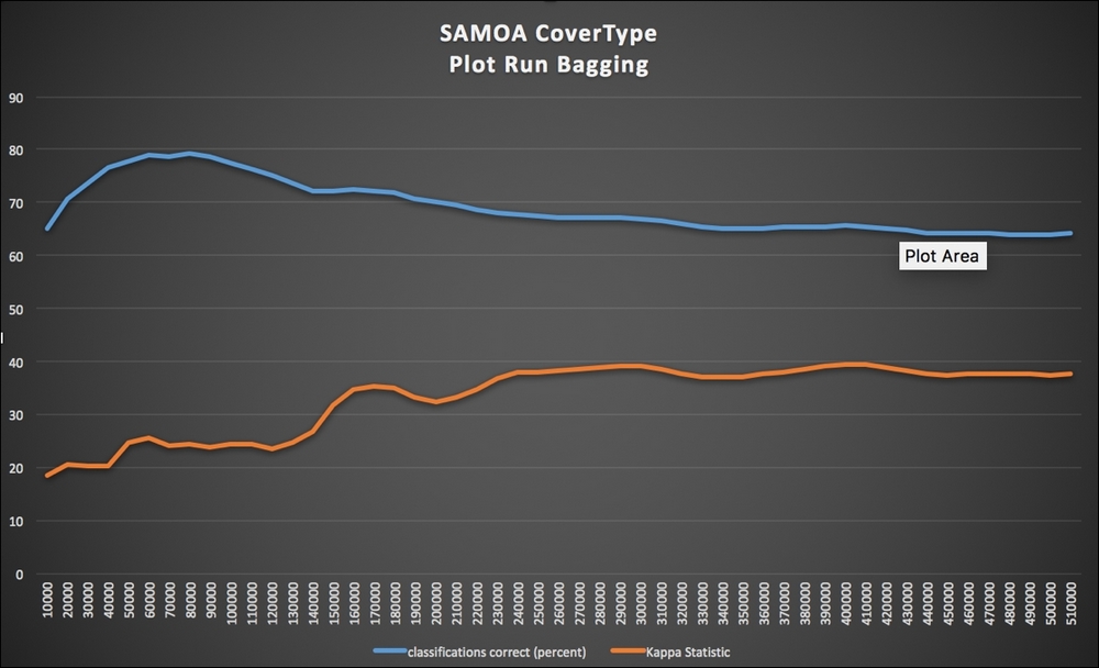
Figure 25: Bagging model performance
When running with Storm, this is the command line:
bin/samoa storm target/SAMOA-Storm-0.3.0-SNAPSHOT.jar "PrequentialEvaluation -l classifiers.ensemble.Bagging
    -s (ArffFileStream -f covtype-train.csv.arff) -f 10000"
The results of experiments using SAMOA as a stream-based learning platform for Big Data are given in Table 5.
|
Algorithm |
Best Accuracy |
Final Accuracy |
Final Kappa Statistic |
Final Kappa Temporal Statistic |
|---|---|---|---|---|
|
Bagging |
79.16 |
64.09 |
37.52 |
-69.51 |
|
Boosting |
78.05 |
47.82 |
0 |
-1215.1 |
|
VerticalHoeffdingTree |
83.23 |
67.51 |
44.35 |
-719.51 |
|
AdaptiveBagging |
81.03 |
64.64 |
38.99 |
-67.37 |
Table 5: Experimental results with Big Data real-time learning using SAMOA
From an analysis of the results, the following observations can be made:
- Table 5 shows that the popular non-linear decision tree-based VHDT on SAMOA is the best performing algorithm according to almost all the metrics.
- The adaptive bagging algorithm performs better than bagging because it employs Hoeffding Adaptive Trees in the implementation, which are more robust than basic online stream bagging.
- The online boosting algorithm with its dependency on the weak learners and no adaptability ranked the lowest as expected.
- The bagging plot in Figure 25 shows a nice trend of stability achieved as the number of examples increased, validating the general consensus that if the patterns are stationary, more examples lead to robust models.
The impact of Machine Learning on businesses, social interactions, and indeed, our day-to-day lives today is undeniable, though not always immediately obvious. In the near future, it will be ubiquitous and inescapable. According to a report by McKinsey Global Institute published in December 2016 (References [15]), there is a vast unexploited potential for data and analytics in major industry sectors, especially healthcare and the public sector. Machine Learning is one of the key technologies poised to help exploit that potential. More compute power is at our disposal than ever before. More data is available than ever before, and we have cheaper and greater storage capacity than ever before.
Already, the unmet demand for data scientists has spurred changes to college curricula worldwide, and has caused an increase of 16% a year in wages for data scientists in the US, in the period 2012-2014. The solution to a wide swathe of problems is within reach with Machine Learning, including resource allocation, forecasting, predictive analytics, predictive maintenance, and price and product optimization.
The same McKinsey report emphasizes the increasing role of Machine Learning, including deep learning in a variety of use cases across industries such as agriculture, pharma, manufacturing, energy, media, and finance. These scenarios run the gamut: predict personalized health outcomes, identify fraud transactions, optimize pricing and scheduling, personalize crops to individual conditions, identify and navigate roads, diagnose disease, and personalize advertising. Deep learning has great potential in automating an increasing number of occupations. Just improving natural language understanding would potentially cause a USD 3 trillion impact on global wages, affecting jobs like customer service and support worldwide.
Giant strides in image and voice recognition and language processing have made applications such as personal digital assistants commonplace, thanks to remarkable advances in deep learning techniques. The symbolism of AlphaGO's success in defeating Lee Sedol, alluded to in the opening chapter of this book, is enormous, as it is a vivid example of how progress in artificial intelligence is besting our own predictions of milestones in AI advancement. Yet this is the tip of the proverbial iceberg. Recent work in areas such as transfer learning offers the promise of more broadly intelligent systems that will be able to solve a wider range of problems rather than narrowly specializing in just one. General Artificial Intelligence, where AI can develop objective reasoning, proposes a methodology to solve a problem, and learn from its mistakes, is some distance away at this point, but check back in a few years and that distance may well have shrunk beyond our current expectations! Increasingly, the confluence of transformative advances in technologies incrementally enabling each other spells a future of dizzying possibilities that we can already glimpse around us. The role of Machine Learning, it would appear, is to continue to shape that future in profound and extraordinary ways. Of that, there is little doubt.
The final chapter of this book deals with Machine Learning adapted to what is arguably one of the most significant paradigm shifts in information management and analytics to have emerged in the last few decades—Big Data. Much as many other areas of computer science and engineering have seen, AI—and Machine Learning in particular—has benefited from innovative solutions and dedicated communities adapting to face the many challenges posed by Big Data.
One way to characterize Big Data is by volume, velocity, variety, and veracity. This demands a new set of tools and frameworks to conduct the tasks of effective analytics at large.
Choosing a Big Data framework involves selecting distributed storage systems, data preparation techniques, batch or real-time Machine Learning, as well as visualization and reporting tools.
Several open source deployment frameworks are available including Hortonworks Data Platform, Cloudera CDH, Amazon Elastic MapReduce, and Microsoft Azure HDInsight. Each provides a platform with components supporting data acquisition, data preparation, Machine Learning, evaluation, and visualization of results.
Among the data acquisition components, publish-subscribe is a model offered by Apache Kafka (References [8]) and Amazon Kinesis, which involves a broker mediating between subscribers and publishers. Alternatives include source-sink, SQL, message queueing, and other custom frameworks.
With regard to data storage, several factors contribute to the proper choice for whatever your needs may be. HDFS offers a distributed File System with robust fault tolerance and high throughput. NoSQL databases also offer high throughput, but generally with weak guarantees on consistency. They include key-value, document, columnar, and graph databases.
Data processing and preparation come next in the flow, which includes data cleaning, scraping, and transformation. Hive and HQL provide these functions in HDFS systems. SparkSQL and Amazon Redshift offer similar capabilities. Real-time stream processing is available from products such as Storm and Samza.
The learning stage in Big Data analytics can include batch or real-time data.
A variety of rich visualization and analysis frameworks exist that are accessible from multiple programming environments.
Two major Machine Learning frameworks on Big Data are H2O and Apache Spark MLlib. Both can access data from various sources such as HDFS, SQL, NoSQL, S3, and others. H2O supports a number of Machine Learning algorithms that can be run in a cluster. For Machine Learning with real-time data, SAMOA is a big data framework with a comprehensive set of stream-processing capabilities.
The role of Machine Learning in the future is going to be a dominant one, with a wide-ranging impact on healthcare, finance, energy, and indeed on most industries. The expansion in the scope of automation will have inevitable societal effects. Increases in compute power, data, and storage per dollar are opening up great new vistas to Machine Learning applications that have the potential to increase productivity, engender innovation, and dramatically improve living standards the world over.
- Matei Zaharia, Mosharaf Chowdhury, Michael J. Franklin, Scott Shenker, Ion Stoica:Spark: Cluster Computing with Working Sets. HotCloud 2010
- Matei Zaharia, Reynold S. Xin, Patrick Wendell, Tathagata Das, Michael Armbrust, Ankur Dave, Xiangrui Meng, Josh Rosen, Shivaram Venkataraman, Michael J. Franklin, Ali Ghodsi, Joseph Gonzalez, Scott Shenker, Ion Stoica:Apache Spark: a unified engine for Big Data processing. Commun. ACM 59(11): 56-65 (2016)
- Apache Hadoop: https://hadoop.apache.org/.
- Cloudera: http://www.cloudera.com/.
- Hortonworks: http://hortonworks.com/.
- Amazon EC2: http://aws.amazon.com/ec2/.
- Microsoft Azure: http://azure.microsoft.com/.
- Apache Flume: https://flume.apache.org/.
- Apache Kafka: http://kafka.apache.org/.
- Apache Sqoop: http://sqoop.apache.org/.
- Apache Hive: http://hive.apache.org/.
- Apache Storm: https://storm.apache.org/.
- H2O: http://h2o.ai/.
- Shahrivari S, Jalili S. Beyond batch processing: towards real-time and streaming Big Data. Computers. 2014;3(4):117–29.
- MGI, The Age of Analytics–—Executive Summary http://www.mckinsey.com/~/media/McKinsey/Business%20Functions/McKinsey%20Analytics/Our%20Insights/The%20age%20of%20analytics%20Competing%20in%20a%20data%20driven%20world/MGI-The-Age-of-Analytics-Full-report.ashx.