
In the previous chapters we spoke about analyzing malware samples both statically and dynamically. From the analysis techniques we discussed, we might be able to derive most of the times if a sample file is malware or not. But sometimes malware may not execute in the malware analysis environment, due to various armoring mechanisms implemented inside the malware sample to dissuade analysis and even detection. To beat armoring mechanisms you want to figure out the internals of the malware code so that you can devise mechanisms to bypass them.
Take another use-case. There are certain other times, where even though via static and dynamic analysis you can figure out if a sample is malware or not, you might still need to know how the malware has been coded internally. This is especially true if you are an antivirus engineer who needs to implement a detection mechanism in your antivirus product to detect the said sample. For example, you might want to implement a decryptor to decrypt files encrypted by a ransomware. But how can you do that? How you provide the decryption algorithm or in other words reverse the encryption algorithm used by a ransomware? We again stand at the same question. Where do we find the code that is used by the malware/ransomware to encrypt the files? The malware author is not going to hand over the malware code to us. All we have in our hand is a piece of malware executable.
And this is where reverse engineering comes in, using which we can dissect malware and understand how it has been programmed. Before we get into reversing malware samples, we need to understand the basics of machine and assembly instructions, debugger tools available and how to use them, identifying various high-level programming constructs in assembly code and so forth, all of this which we cover in this chapter, laying the foundation to learn more advanced reversing techniques and tricks in the next few chapters in this Part 5 of the book.
Reversing and Disassemblers: Source ➤ Assembly ➤ Back

Process of creating executable files from high-level languages using a compiler
The malware executable files we receive are all in the machine code format, as seen on the right side of the figure. Since it is hard, if not impossible, to understand what the malware or executable is functioned to do by looking at this machine code, we use reverse engineering, which is a process of deriving back high-level pseudocode from machine code to gain an understanding of the code’s intention.
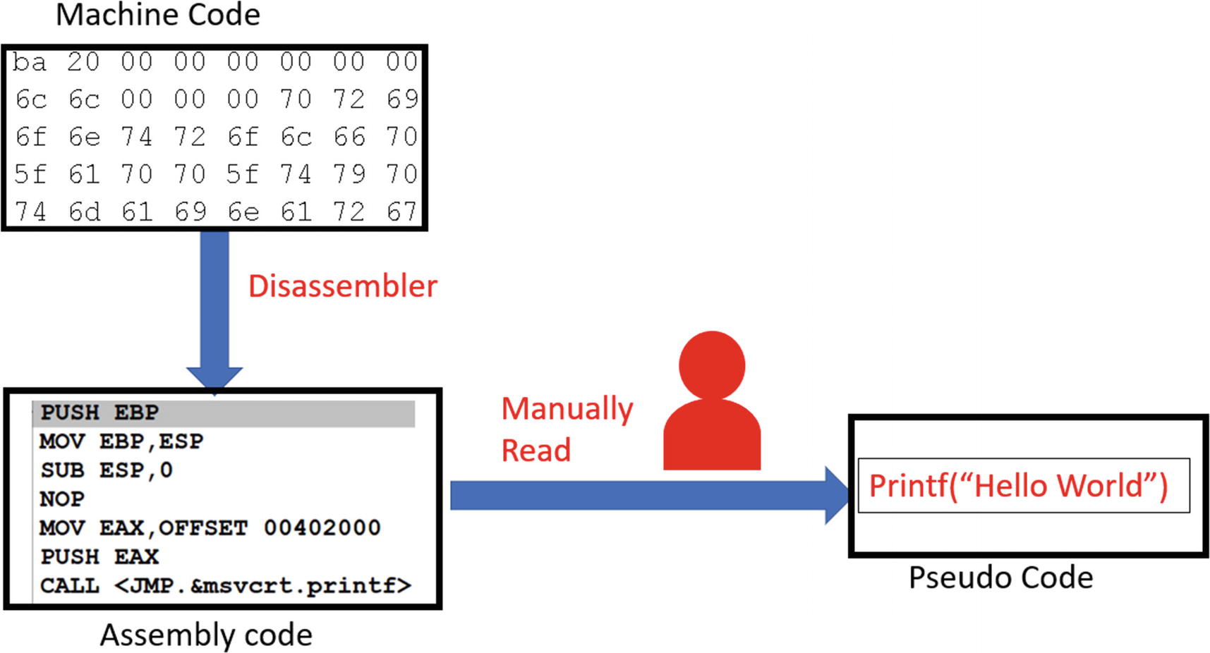
Reverse engineering process that involves converting machine code to a more human-readable assembly language format
Malware reverse engineers also use other tools like decompilers to convert the machine code into a high-level language pseudo-code format that is even easier to read. A good example of these decompilers is the Hex-Rays decompiler that comes with the IDA Pro, and the Sandman decompiler, which comes integrated with debuggers like x64Dbg.
But the main tool involved in the reversing process is still the disassembler that converts the code into assembly language. So, to be a good reverse engineer, a thorough understanding of assembly language and its various constructs is important, along with the ability to use various disassembly and debugging tools.
In the next set of sections, we go through a brief tutorial of the x86 architecture and understand various assembly language instructions that should set our fundamentals up for reversing malware samples.
PE and Machine Code
There are many processor families like Intel, AMD, PowerPC, and so forth. We spoke about machine code being generated by the compiler, where the generated machine code is instruction code that can be understood by the CPU on the system. But there are many processor families, and each of them might support a machine code instruction set that only they can understand.
So, machine code generated for one instruction set only runs on those CPUs/processors that understand that machine code instruction set. For example, an executable file containing machine code that has been generated for the PowerPC machine code instruction set won’t run on Intel/AMD CPUs that understand the x86 instruction set and vice versa.
Let’s tie this to our PE file format used by Windows OS. In Chapter 4, we spoke about PE files, where if you want to create an executable program for Windows OS, we need to compile the program source into a PE file that follows the PE file format. The PE file format has the machine code embedded within it in one or multiple of its sections. For example, it can be in the .text section. Using the PE file format structure, Windows can locate the machine code in the file, extract it, and then execute it on the CPU. But how does the Windows system know that the machine code in the PE file is meant for the CPU/processor type of that system? It does this using the Nt Headers ➤ File Header ➤ Machine field in the PE header of the file.

The Machine field in the file header of the PE file Format for Sample-4-1 that indicates the processor type meant to run this PE file
x86 Assembly Language
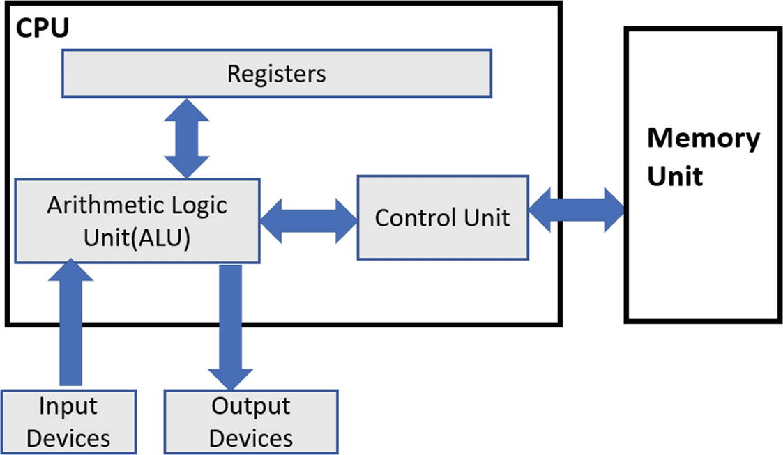
The Von Neumann computer architecture
The CPU, or the processor
The memory
The input/output devices
Input and output devices
These are the devices from which the computer either receives data or sends data out. A good example of these devices is display monitors, keyboard, mouse, disk drives like HDD/SSD, CD drives, USB devices, network interface cards (NICs), and so forth.
Memory
Memory is meant to store instructions (code) that are fetched and executed by the CPU. The memory also stores the data required by the instructions to execute.
CPU
The CPU is responsible for executing instructions; that is, the machine code of programs. The CPU is made up of the arithmetic logic unit (ALU), control unit, and the registers. You can think of the registers as a temporary storage area used by the CPU to hold various kinds of data that are referenced by the instructions when they are executed.
Memory stores both the instructions (code) and the data needed by the instructions. The control unit in the CPU fetches the instructions from the memory via a register (instruction pointer), and the ALU executes them, placing the results either back in memory or a register. The output results from the CPU can also be sent out via the input/output devices like the display monitor.
From a reverse engineering point of view, the important bits we need to learn are the registers, the various instructions understood and executed by the CPU, and how these instructions reference the data in the memory or the registers.
Instruction: The Format
Needless to say, when we are talking about instructions in this chapter, we mean assembly language instructions . Let’s learn the basic structure.
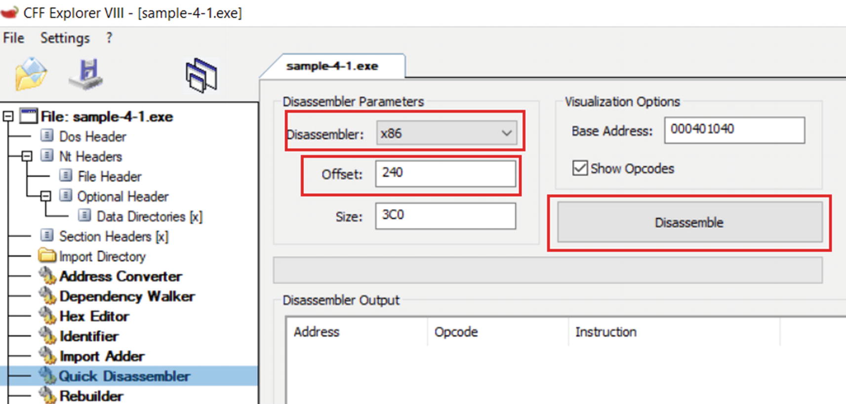
The Quick Disassembler option in CFF that disassembles the machine code into assembly language instructions
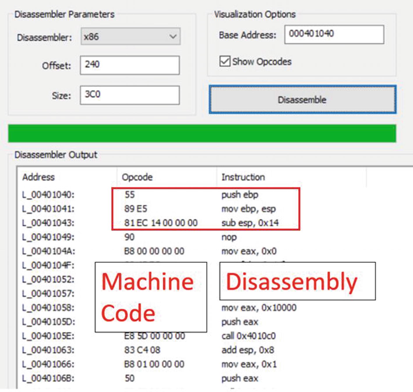
The disassembled instructions for Sample-4-1.exe viewed using CFF Explorer
There are three columns. The middle column, Opcode, holds the machine code, which, if you read, looks like garbage. But the disassembler decodes these machine code, separating the instructions and providing you a human-friendly readable format for them in the assembly language seen in the third column, Instruction.
Break Up of the Machine Code Bytes in Sample-4-1 That Consists of 3 Instructions
Opcodes and Operands
Now the representation of what an opcode means in the listing and figure might be slightly different or rather loose. But to be very precise, every instruction consists of an opcode (operation code) and operands. Opcode indicates the action/operation of the instruction that the CPU executes, and the operands are data/values that the operation operates on.
Break Up of the 3 Instructions into Opcode/Actions and Operands
So, while referring to documents, manuals, and disassembler output, be ready to understand the context and figure out what it refers to as opcode.
Operand Types and Addressing Mode
Immediate operands are fixed data values. Listing 16-3 shows some examples of instructions where the operands are immediate. The 9 is a fixed value that the instruction operates on.
Example of Instructions That Uses Both Immediate and Register Operands
Register operands are registers like EAX, EBX, and so forth.
In Listing 16-3, you can see that both the instructions take operands EAX and ECX, which are registers. You can also see that the same instructions also take immediate operands. Instructions can take operands of multiple types based on how the instruction has been defined and what operands it can operate on.
Indirect memory addresses provide data values that are located at memory locations, where the memory location can be supplied as the operand through a fixed value, register, or any combination of register and fixed value expression, which disassemblers show you in the form of square brackets ([]), as seen in Listing 16-4.
Example of Instructions That Uses Operands in the Form of Indirect Memory Address
Implicit vs. Explicit Operands
As you learned, we have operands which the instruction operates on. These operands that an instruction operates on can be either specified explicitly along with the instruction opcode or can be assumed implicitly based on the definition of the instruction.
For example, the instruction PUSH [0x40004] explicitly specifies one of its operands, which is the memory operand 0x40004. Alternatively, PUSHAD doesn’t take any other explicit operands. Its other operands are implicitly known. This instruction works by pushing various registers (i.e., implicit operands) to the stack, and these registers which it pushes to the stack are known implicitly based on the function defined for this instruction.
Endianness
Endianness is the way to order or sequence bytes for any data in memory. For example, consider the number 20, which, when represented using bytes, is represented in hex as 0x00000014. To store this value in memory, these individual bytes 0x00, 0x00, 0x00, 0x14 can either be stored in memory addresses that start at a lower address and move to a higher address or the other way round.
The method where the bytes of a value are stored in a format where the least significant byte is stored at the lowest address in a range of addresses used to store the value is called little-endian representation.
The method where the bytes of a value are stored in the format where the most significant byte is stored at the lowest address in a range of addresses used to store the value is called big-endian representation.
For example, from Listing 16-1, the third instruction is present in the memory as 89 EC 14 00 00 00. This machine code translates to sub esp,0x14, which is the same as sub esp,0x00000014. 14 00 00 00 is the order in memory, where the 14 is held in the lowest/smallest address in memory. But we have compiled this piece of sample code for x86 little-endian processors. Hence, when the processor and even the disassemblers and the debuggers convert it, they read the data values in the little-endian format, which is why it is disassembled into 0x00000014.
These days most x86-based processors use the little-endian format. But you might come across samples that might have been compiled for different processor types that might use the big-endian format. Always watch out for the endianness used by the processor type you are reversing/analyzing samples for. You don’t want to get caught out reading values in the wrong order.
Registers
Data registers
Pointer register
Index register
Control/flags register
Debug registers
Segment registers

The various categories of x86 registers
Data Registers

Data register EAX split up into 16- and 8-bit sections that can be referred individually
EAX
This register is also called the accumulator and is popularly used to store results from the system. For example, it is widely used to hold the return values from subroutines/functions.
EBX
Called the base register, it is used by instructions for indexing/address calculation. We talk about indexing later.
ECX
Called the counter register. Some of the instructions, like REP, REPNE, and REPZ, rely on the value of ECX as a counter for loops.
EDX
Also used for various data input/output operations and used in combination with other registers for various arithmetic operations.
Do note that the specific functionalities are not set in stone, but most of the time, compilers generate instructions that end up using these registers for these specific functionalities. End of the day, these are general-purpose registers used by instructions for various purposes.
Pointer Registers
EIP
EIP is a special-purpose pointer register called the instruction pointer. It holds the address of the next instruction to be executed on the system. Using the address pointed to by the EIP, the CPU knows the address of the instruction it must execute. Post execution of the instruction, the CPU automatically update the EIP to point to the next instruction in the code flow.
ESP
This is the stack pointer and points to the top of the stack (covered later when we talk about stack operations) of the currently executing thread. It is altered by instructions that operate on the stack.
EBP
Known as the base pointer, it refers to the stack frame of the currently executing subroutine/function. This register points to a particular fixed address in the stack-frame of the currently executing function, which allows us to use it as an offset to refer to the address of the various other variables, arguments, parameters that are part of the current function’s stack-frame.
EBP and ESP both enclose the stack frame for a thread in the process, and both can access local variables and parameters passed to the function, which are held in the function’s stack-frame.
Index Registers
ESI and EDI are the two index registers which point to addresses in memory, for the means of indexing purposes. The ESI register is also called the source index register, and the EDI is also called the destination index register , and are mostly used for data transfer related operations like transferring content among strings and arrays and so forth.

Example use-case of ESI and EDI used for transferring data across memory

ESI and EDI registers can be split into 16 bits, and the lower 16 bit part referred to as SI and DI respectively

eflags register
Flags (Status) Register
The flags register is a single 32-bit register that holds the status of the system after running an instruction. The various bits in this register indicate various status conditions, the important ones being CF, PF, AF, ZF, SF, OF, TF, IF, and DF, which can be further categorized as status bits and control bits. These bit fields occupy nine out of thirty-two bits that make up the register, as seen in Figure 16-11.
Description of the Various Status Bit Fields in the Flags Register
Flags Bit | Description |
|---|---|
Carry flag (CF) | Indicates a carry or a borrow has occurred in mathematical instruction. |
Parity flag (PF) | The flag is set to 1 if the result of an instruction has an even number of 1s in the binary representation. |
Auxiliary flag (AF) | Set to 1 if during an add operation, there is a carry from the lowest four bits to higher four bits, or in case of a subtraction operation, there is a borrow from the high four bits to the lower four bits. |
Zero flag (ZF) | This flag is set to 1 if the result of an arithmetic or logical instruction is 0. |
Sign flag (SF) | The flag is set if the result of a mathematical instruction is negative. |
Overflow flag (SF) | The flag is set if the result of an instruction cannot be accommodated in a register. |
ADD/SUB/CMP/MUL/DIV instructions affect all six flags
INC/DEC affect all the flags, except the CF flag
Data movement instructions like MOV do not affect the flags register
Description of the Various Control Bit Fields in the Flags Register
Flags | Description |
|---|---|
Trap flag (TF) | If the flag is set to 1, debuggers can debug a program in the CPU. |
Interrupt flag (IF) | This flag decides how the CPU should deal with hardware interrupts. |
Direction flag (DF) | The flag is used by string instructions like MOVS, STOS, LODS, SCAS to determine the direction of data movement. |
Debug Register
The debug registers DR0-DR7 are meant for debugging purposes. The debug registers DR0-DD3 are used for storing addresses where hardware breakpoints (covered later under debuggers) are placed, while the type of hardware breakpoint placed is specified in the bits in the DR7 register.
Important x86 Instructions
Intel has 1500+ x86 instructions, and it’s not possible to memorize each of those. Add to that the specialized instruction sets like SSE, MMX, AVX, and so forth, and the list of instructions gets bigger. From a reverse engineering perspective, we need to learn the most basic instructions, and as and when we come across new instructions, it does you good to look them up in Intel’s instructions reference manual to understand what they do.
Stack operation instructions
Arithmetic instructions
Logical instructions
Control flow instructions
Data movement instructions
Address loading instructions
String manipulation instructions
Interrupt instructions
Stack Operations
A stack is a memory area that is used by programs to store temporary data related to function calls. The two most basic instructions that manipulate the stack are PUSH and POP. There are other instructions as well, like the CALL and RET that manipulate the stack, which is important as well, which we talk about later. Apart from these, there are other stack manipulation instructions like ENTER and LEAVE, which you can read about using Intel’s reference manual.
General Format of PUSH and POP Instructions
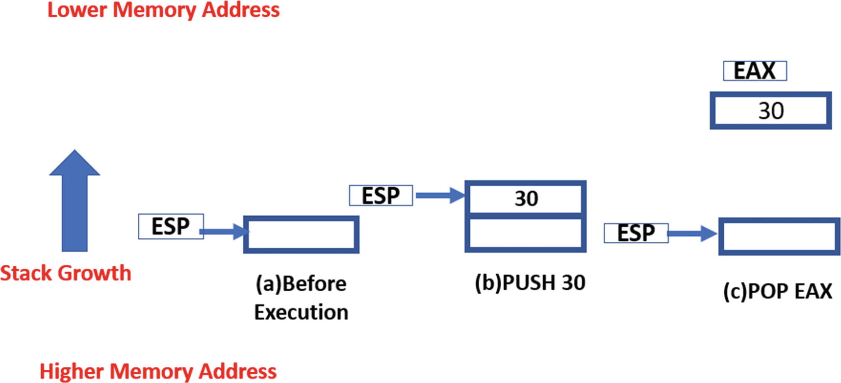
Illustration of how the stack grows when data is pushed and popped from it
Similarly, when a POP is executed, the address in ESP is automatically incremented by 4, simulating popping/removal of data from the stack. For example, if the ESP is 0x40000, a POP instruction copy the contents at address 0x40000 into the operand location and increments ESP to 0x40004.
As an example, have a look at Figure 16-12 that shows how the stack expands and contracts and the way ESP pointer moves when PUSH and POP instructions are executed.
There are other variations of the PUSH instruction like PUSHF and PUSHFD, which don’t require an explicit operand that it pushes onto the stack, as these instructions implicitly indicate an operand: the flags register. Both save the flags registers to the stack. Similarly, their POP instruction counterparts have variants POPF and POPFD, which pop the data at the top of the stack to the flag registers.
Arithmetic Instructions
Arithmetic instructions perform mathematical operations on the operands, including addition, subtraction, multiplication, and division. While executing mathematical instructions, it’s important to watch out for changes in the flag registers.
Basic Arithmetic Instructions
ADD, SUB, MUL, and DIV are the basic arithmetic instructions.
ADD instruction adds two operands using the format ADD <destination>, <source>, which translates to <destination> = <destination> + <source>. The <destination> operand can either be a register or an indirect memory operand. The <source> can be a register, immediate value, or an indirect memory operand. The instruction works by adding the contents of the <source> to the <destination> and storing the result in the <destination>.
SUB instruction works similarly to the ADD instruction, except that it also modifies the two flags in the flags register: the zero flag (ZF) and the carry flag (CF) . The ZF is set if the result of the subtraction operation is zero, and the CF is set if the value of the <destination> is smaller in value than the <source>.
Some Examples of ADD and SUB Instructions and What They Mean
MUL instruction like the name indicates multiples its operands—the multiplicand and the multiplier, where the multiplicand is an implicit operand supplied via the accumulator register EAX, and hence uses the format MUL <value>, which translates to EAX = EAX * <value>. The operand <value> can be a register, immediate value, or an indirect memory address. The result of the operation is stored across both the EAX and the EDX registers based on the size/width of the result.
DIV instruction works the same as the MUL instruction, with the dividend supplied via the implicit operand: the EAX accumulator register and the divisor supplied via an immediate, register, or an indirect memory operand. In both the MUL and DIV instructions cases, before the instruction is executed, you see the EAX register being set, which might appear either immediately before the MUL or DIV instruction or, in some cases, might be further back. Either way, while using the debugger like OllyDbg, you can check the live value of the EAX register just before these instructions execute so that you know what the operand values are.
MUL Instruction That Multiplies 3 and 4
Increment and Decrement Instructions
The increment instruction (INC) and the decrement instruction (DEC) take only one operand and increment or decrement its content by 1. The operand may be an indirect memory address or a register. The INC and DEC instruction alter the five flag bits in the flags register: AF, PF, OF, SF, and ZF.
Various Examples of INC and DEC Instructions and What They Translate to
Logical Instructions
AND, OR, XOR, and TEST are the basic arithmetic operations supported by x86. All the instructions take two operands, where the first operand is the destination, and the second is the source. The operation is performed between each bit in the destination and each bit of source, and the result is stored in the destination.
AND instruction logically ANDs two operands using the format AND <destination>, <source>. The AND operation is performed between the corresponding bit values in the source and destination operands. The <destination> operand can either be a register or an indirect memory operand. The <source> can be a register, immediate value, or an indirect memory operand. Both <destination> and <source> cannot be in memory at the same time.
OR and XOR instructions work in the same way except the operation is performed between the individual bit fields in the operands supplied to these instructions. OF and CF flags are set to 0 by all three instructions. ZF, SF, and PF flags are also affected by the result.
Examples of AND and XOR Instructions
Shift Instructions
The logical shift shifts the bits in an operand by a specific count, either in the left or right direction. There are two shift instructions: the left-Shift (SHL) and the right-Shift (SHR).
The SHR instruction follows the following format, SHR <operand>,<num>. The <operand> is the one in which the instruction shifts the bits in a specific direction, and it can be a register or memory operand. The <num> tells the operand how many bytes to shift. The <num> operand value can be either an immediate value or supplied via the CL register.

Example of how a SHR instruction shifts the contents of its operand
Similarly, the SHL instruction shifts every bit of its operand in the left direction. As a result, the leftmost bit is pushed out of AL, which is stored in CF. The void in the rightmost bit(s) is filled with a value of 0.
If you go back to the example in the figure, the decimal equivalent of the content of AL register is 1011; that is, the value 11 before the right-Shift. If you shift it right by 1, the value is 101; that is, 5. If you again execute the same instruction moving it right by 1 bit field value, it becomes 10; that is, 2. As you can see every right-Shift divides the value of the contents you are right-Shifting by 2 and this is what SHR does and it is used a lot. If you generalize it into a mathematical formula , a SHR <operand>,<num> is equivalent to <operand> = <operand>/(2 ^^ <num>).
Similarly, the SHL instruction also works in the same manner as, except that every left-Shift multiplies the content you are shifting by a value of 2. If you generalize it into a mathematical formula, a SHL <operand>, <num> is equivalent to <operand> = <operand> * (2 ^^ <num>).
Rotate Instructions

Example of how a ROR instruction rotates the contents of its operand
The format of Rotate instructions is similar to shift instruction. We have two rotate instructions ROR and ROL. Rotate Right; that is, ROR follows the format ROR <operand>, <num> and the ROL instruction follows the format ROL <operand>, <num>. Again <operand> and <num> mean the same as in SHR instruction.
Comparison Instructions
The two instructions CMP and TEST are used for the comparison of two operands. They are generally used in combination with conditional execution and branching instructions like the conditional JUMP instructions. These instructions are among the most encountered instructions while debugging, and open whenever you implement loops, if/else conditions, switch cases in your high-level language.
The general format of these instructions is CMP <destination>, <source> and TEST <destination>, <source>. The <destination> operand can be a register or an indirect memory address operand, and the <source> can be either an immediate or a register operand. Though we have called the operands <source> and <destination> neither of these operand values are modified. Instead both instructions update the various status fields in the flags register.
Example of the Various Operand Values Used with TEST and CMP Affecting the Flags Register
CMP <destination> <source> | ZF | CF |
|---|---|---|
destination == source | 1 | 0 |
destination < source | 0 | 1 |
destination > source | 0 | 0 |
TEST <destination> <source> | ZF | |
destination & source == 0 | 1 | |
destination & source != 0 | 0 |
Control Flow Instructions
The Control Flow Instructions alter the linear flow of the execution of the instructions in a program. These instructions come up in assembly as a result of using loops and if/else branches, switch statements, goto in high-level languages which we generally used to branch/modify the execution path of the program based on various conditions. The general format of any control flow instruction takes a <target address> as its operand to which it transfer/branch its execution post its execution.
Control flow instructions can largely be categorized as conditional branch and unconditional branch instructions, which we cover in the next set of sections.
Unconditional Branch Instructions
An unconditional branch instruction like the name says unconditionally branches out and transfers control of the execution of the process to the target address. The three most popular unconditional branch instructions are CALL, JMP and RET.
The JMP instruction follows the format jmp <target_address>, where the operand <target_address> is the target address of the instruction, which can either be a register, absolute immediate value, or an indirect memory address. When this instruction executes the EIP is set to the <target_address> transferring execution control of the program to this <target_address>.

CALL instruction transfers execution control to its target address and stores the return address on the stack where it resumes execution when execution control returns back
As you can see in the figure, on the left side of the figure, the currently executing instruction at Addr_3, which is the CALL instruction when executed transfer control to the target Addr_33. After execution of this CALL instruction, EIP is set to Addr_33 transferring control of the program to the instruction at this address. Also, the address of the next instruction after the CALL instruction Addr_4 is pushed to the stack, which is the return address.
Now when the control (EIP) reaches the RET instruction at Addr_36, and it gets executed, the CPU update the EIP with the value at the top of the stack pointed to by the ESP, and then increments the ESP by 4 (basically popping/removing the value at the top of the stack). Hence you can say after executing the RET instruction, the control goes to the address that is pointed to by the ESP.
Do note that unlike a CALL instruction, a jump instruction does not push the return address to the stack.
Conditional Branch Instructions
A conditional branch instruction uses the same general format as its unconditional counterpart, but it jumps to its <target_address> only if certain conditions are met. The various jump conditions that need to be satisfied by these instructions are present in the various status flags of the flags register. The jump conditions are usually set by CMP, TEST, and other comparison instructions, which are executed before these conditional branch instructions are executed.
Various Conditional Branch Instructions and the Flags They Need Set To Make A Jump
Instruction | Description |
|---|---|
JZ | Jumps if ZF is 1 |
JNZ | Jumps if ZF is 0 |
JO | Jumps if OF is 1 |
JNO | Jumps if OF is 0 |
JS | Jumps if SF is 1 |
JNS | Jumps if SF is 0 |
JC | Jumps if CF is 1 |
JNC | Jumps if CF is 0 |
JP | Jumps if PF is 1 |
JNP | Jumps if PF is 0 |
Loops
Loops are another form of control flow instruction that loop or iterate over a set of instructions by using a counter set in one of its implicit operands, the ECX register. A loop instruction uses the following format: LOOP <target_address>. Before the loop can start, the ECX register is set with the loop count value, which defines the iterations that the loop needs to run. Every time the LOOP instruction executes, it decrements the ECX register (the counter) by 1 and jumps to the <target_address> until the ECX register reaches 0.
You may encounter other variations of the LOOP instructions LOOPE, LOOPZ, LOOPNE, and LOOPNZ. The instructions LOOPE/LOOPZ iterates till ECX is 0 and ZF flag is 1. The instructions LOOPNE/LOOPNZ iterates till ECX is 0 and ZF is 1.
Address Loading Instructions
Examples of LEA Address Loading Instructions and What They Translate To
Instruction | Description |
|---|---|
LEA EAX, [30000] | EAX = 30000 |
LEA EAX, [EDI + 0x30000] | Assuming EDI is currently set to 0x40000EAX = 0x40000 + 0x30000EAX = 0x70000 |
After the address is loaded into the register, the register can be used by other instructions that need to refer to the data at the address or refer to the memory address itself.
Data Movement Instructions
Data movement instructions are meant to transfer data from one location to another. Let’s start by looking at some of the popular data movement instructions, starting with the most frequently encountered one MOV.
Examples of MOV Instructions and What They Translate To
Instruction | Meaning |
|---|---|
MOV EAX, 9 | EAX = 9 |
MOV [EAX], 9 | [EAX] = 9 |
MOV EAX, EBX | EAX = EBX |
MOV [EAX], EBX | [EAX] = EBX |
MOV [0x40000], EBX | [0x40000] = EBX |
MOV EAX, [EBX + 1000] | EAX = [EBX + 1000] |
You see the braces [ ] in a lot of instructions. The square brackets indicate the content of the address in a MOV instruction, but for instructions like LEA, it indicates the address as the value itself that is moved to the destination.
MOV EAX, [30000] -> moves contents located at address 30000 to EAX register
But LEA EAX,[30000] -> set the value of EAX to 30000
The XCHG instruction is also another data movement instruction, that exchanges data between its operands. its format is like the MOV instruction: XCHG <destination>, <source>. The <destination> and <source> can be a register or an indirect memory address, but they can’t be indirect memory addresses at the same time.
String Related Data Movement Instructions
In the previous section, we saw the MOV instruction. In this section, we look at some other instructions that are related to data movement but, more specifically, that comes up in assembly due to the use of string related operations in higher-level languages. But before we get to that, let’s explore three very important instructions CLD, STD, and REP that are used in combination with a lot of this data and string movement instructions.
CLD instruction clear the direction flag (DF); that is, set it to 0, while STD instruction works the opposite of CLD and sets the direction flag (DF); that is, set it to 1. These instructions are generally used in combination with other data movement instructions like MOVS, LODS, STOS since these instructions either increment or decrement their operand values based on the value of the DF. So, using the CLD/STD instruction, you can clear/set the DF, thereby deciding whether the subsequent MOVS, LODS, STOS instructions either decrement or increment their operand values. We cover examples for this shortly.
How REP Repeats Execution of Other Instructions Using the Counter Value in ECX
There are other variations of the REP instruction—REPE, REPNE, REPZ, REPNZ, which repeat based on the value of the status flags in the flag register along with the counter value held in the ECX register. We are going to continue seeing the usage of REP in the next section.
MOVS
The MOVS instruction , like the MOV instruction, moves data from the <source> operand to the <destination> operand, but unlike MOV, the operands are both implicit. The <source> and <destination> operands for MOVS are memory addresses located in the ESI/SI and EDI/DI registers, respectively, which need to be set before MOVS instruction is executed. There are other variants of the MOVS instruction based on the size of the data; it moves from the <source> to the <destination>: MOVSB, MOVSW, and MOVSD.
No operands are needed as operands are implicit, with ESI/SI used as <source> and EDI/DI used as <destination>. Both register operands need to be set before MOVS instruction is executed.
Moves data from the address pointed to by ESI to address pointed to by EDI.
Increments both ESI/SI and EDI/DI if DF is 0, else decrements it.
Increments/decrements the ESI/EDI value by either a BYTE, WORD, or DWORD based on the size of data movement.
Now let’s stitch it all together. MOVS instruction in itself moves data from <source> to <destination>. Its real use is when you want to move multiple data values in combination with the REP instruction. Combine this with CLD/STD, and you can either have MOVS instruction move forward or backward by incrementing/decrementing the address values you have put in ESI/EDI.
Example of MOVSB in Combination with REP That Copies Data from Source to Destination in the Forward Direction, and the Corresponding C Pseudocode for the Assembly
The first two instructions set ESI to memory location 0x30000 and EDI to 0x40000. The next instruction sets ECX to 3, which sets up the counter for the subsequent move operation. The fourth instruction sets the DF flag to 0, indicating that the ESI and EDI address values should be incremented, moving it in the forward direction. Let’s assume that the address x30000 contains data 11 22 33 44. Now, if the instruction REP MOVSB is executed, MOVSB is executed three times as ECX is 3. Each time MOVSB is executed, a byte is moved from the location pointed to by the ESI to the location pointed by EDI. Then ESI and EDI are incremented as the DF flag is set to 0. Also, with the effect of REP, ECX is decremented. After execution of the fifth instruction completes, the address pointed to originally by EDI: 0x40000 now contains 11 22 33.
In the listing, if we replaced CLD in the instructions with STD, then both source and destination decrement instead of being incremented: src-- and dst--.
STOS and LODS
There are other data movement instructions STOS and LODS, which work similarly to the MOVS instruction but using different registers as operands. Both instructions have their variants: STOSB, STOSW, STOSD and LODSB, LODSW, LODSD, which transfer a byte, word, or double word, respectively. The REP instruction works similarly with these instructions as well. Look up these instructions in the intel reference manual or even the web, to check the different operand registers these instructions take when compared to MOVS.
SCAS
SCAS is a string-scanning instruction used to compare the content at the address pointed to by EDI/DI with the content of the EAX/AX/AL accumulator register. This instruction affects the flags register by setting the ZF if a match is found. The instruction also increments EDI/DI if the DF flag is 0, else decrements it. This feature allows it to be used in combination with the REP instruction, allowing you to search a memory block for a character or even compare character strings.
Example of SCAS Searching for Character 'A' in a Memory Block of 1000 Bytes
NOP
NOP stands for no operation, and like the name says, this instruction does nothing, with execution proceeding to the next instruction past this, and absolutely no change to the system state, apart from the EIP incrementing to point to the next instruction. This instruction has an opcode of 0x90 and is very easily noticeable if you are looking directly at the raw machine code bytes. This instruction is commonly used for NOP slides while writing exploits shellcode for buffer overflow and other types of vulnerabilities.
INT
INT instruction is meant to generate a software interrupt. When an interrupt is generated, a special piece of code called the interrupt handler is invoked to handle the interrupt. Malware can use interrupts for calling APIs, as an anti-debugging trick and so forth. INT instruction is called with an interrupt number as an operand. The format of INT instruction is INT <interrupt numbers>. INT 2E, INT 3 are some examples of the INT instruction.
Other Instructions and Reference Manual
In the sections, we went through some of the important and frequently encountered instructions in assembly, but the actual no instructions are far huger in number. Whenever you encounter a new instruction, or when you want to obtain more information about an instruction, searching on the web is a good first step. There are enough resources out there with various examples that should help you understand what an instruction should do and how to use it with various operands.
Intel 64 and IA-32 architectures software developer’s manual volume 1: Basic architecture
Intel 64 and IA-32 architectures software developer’s manual volume 2A: Instruction set reference, A–L
Intel 64 and IA-32 architectures software developer’s manual volume 2B: Instruction set reference, M–U
Intel 64 and IA-32 architectures software developer’s manual volume 2C: Instruction set reference, V–Z
Debuggers and Disassembly
Now that you understand the x86 architecture and the x86 instruction set, let’s explore the process of disassembly and debugging of programs.
As you learned that disassembly is a process of converting the machine code into the more human-readable assembly language format, a lot of which we have seen in the previous section. To disassemble a program, you can use software (also known as disassemblers) that does nothing but disassemble a program (that’s right, it doesn’t debug a program, but only disassembles it). Alternatively, you can also use a debugger for the disassembly process, where a debugger apart from its ability to debug a program can also double up as a disassembler.
For our exercises, we are going to introduce you to two popular debuggers— OllyDbg and IDA Pro—that disassemble the code and present it visually. There are other popular debuggers as well, including Immunity Debugger, x64dbg, Ghidra, and Binary Ninja, all of which are worth exploring.
Debugger Basics
A debugger is software that troubleshoots other applications. Debuggers help programmers to execute programs in a controlled manner, not presenting to you the current state of the program, its memory, its register state, and so forth, but also allowing you to modify this state of the program while it is dynamically executing.
There are two types of debuggers based on the code that needs to be debugged: source-level debuggers and machine-language debuggers . Source-level debuggers debug programs at a high-level language level and are popularly used by software developers to debug their applications. But unlike programs that have their high-level source code available for reference, we do not have the source code of malware when we debug them. Instead, what we have are compiled binary executables at our disposal. To debug them, we use machine language binary debuggers like OllyDbg and IDA, which is the subject of our discussion here and which is what we mean here on when we refer to debuggers.
These debuggers allow us to debug the machine code by disassembling and presenting to us the machine code in assembly language format and allowing us to step and run through this code in a controlled manner. Using a debugger, we can also change the execution flow of the malware as per our needs.
OllyDbg vs. IDA Pro
Now when you launch a program using OllyDbg, by default, the debugger is started. Debugging is like dynamic analysis where the sample is spawned (process created). Hence you see a new process launched with OllyDbg as the parent when you start debugging it with OllyDbg. But when you open a program with IDA by default, it starts as a disassembler, which doesn’t require you to spawn a new process for the sample. If you want to start the debugger, you can then make IDA do it, which spawns a new process for the sample to debug it. Hence IDA is very beneficial if you only want to disassemble the program without wanting to run it. Of course, do note that you can use IDA as a debugger as well.
Also, IDA comes with various disassembly features that let you visualize the code in various styles, one of the most famous and used features being the graph view, that lets you visualize code in the form of a graph. IDA also comes with the Hex-Rays decompiler, which decompiles the assembly code into C style pseudocode that quickly helps you analyze complex assembly code. Add to this the various plugins and the ability to write scripts using IDA Pro, and you have enough malware reverse engineers who swear by IDA Pro. Do note that IDA Pro is software for purchase, unlike OllyDbg and other debuggers, which are free.
OllyDbg is no slouch, either. Although it lacks many of the features that graph view and the decompiler have, it is a simple and great piece of debugging software that most malware reversers use as a go-to tool when reversing and analyzing malware. OllyDbg has lots of shortcuts that help reverse engineers to quickly debug programs. You can create your plugins as well, and best of all, it is free.
There are other debuggers and disassemblers out there, both paid and free, that have incorporated various features of both OllyDbg and IDA Pro. For example, x64Dbg is a great debugger that is free, provides a graph view similar to IDA Pro, and integrates the Sandbox decompiler. Binary Ninja is another great disassembler/debugger. Ghidra is the latest entry to this list. New tools come up every day, and it is best if we are aware of all the latest tools and how to use them. No one debugger or disassembler provides all the best features. You must combine all of them to improve your productivity while reversing malware samples.
Exploring OllyDbg

Enabling OllyDbg option to make it pause/break execution at entry point

SFX settings that need to be unset in OllyDbg Options

Main OllyDbg window that shows other subwindows for a process debugged
Disassembly Window
Displays the disassembled code. As seen in Figure 16-19, this window has four columns. The first column shows the address of the instruction, the second the instruction opcode (machine code), the third column shows assembly language mnemonic for the disassembled opcode, and the fourth column gives a description/comment of the instruction whenever possible. The Disassembly window also highlights the instruction in black for the instruction that is currently going to be executed, which is also obtained by the value of the EIP register.
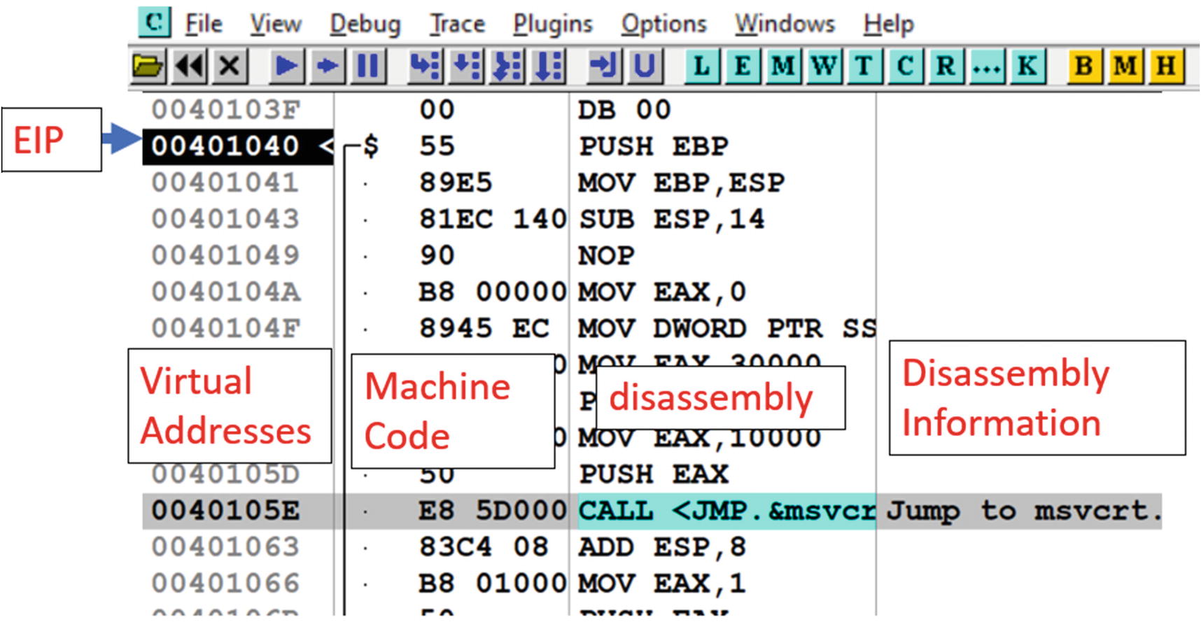
Disassembly window of OllyDbg and its various columns with various bits of info
Register window
Displays the registers and their values, including the flags register.
Information window
Displays information for an instruction you click from the Disassembly window.
Memory window
You can browse the memory and view its content using this window.
Stack window
Displays theaddress and contents of the stack, as seen in Figure 16-20. The current top of the stack; that is, the value in the ESP is highlighted in black in this window. The first column in this window indicates the stack address. The second column displays the data/value at the stack address. The third column displays the ASCII equivalent of the stack value. The last column displays the information/analysis figured by the debugger for the data at that stack address.
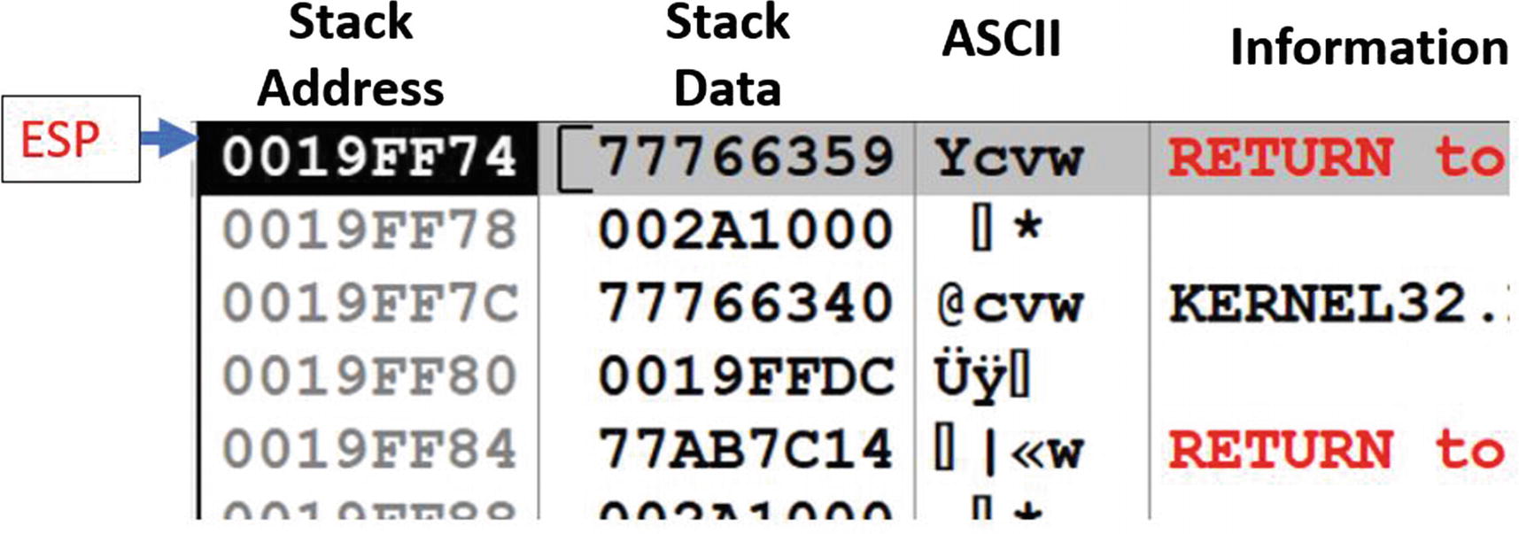
The stack window of OllyDbg and its various columns holding info about the contents of the stack
Basic Debugging Steps

The various fast access buttons in OllyDbg the main menu bar
Hovering the mouse over the button opens a small information message displaying to you what the button does. The same functionality can also be reached using the Debug menu bar option. The following is a description of some of these buttons. Some of the other buttons are described later.
Stepping Into and Stepping Over
Stepping is a method using which we can execute instructions one at a time. There are two ways to step through instructions: step over and step into. Both when used work in the same way, unless a CALL instruction is encountered. A CALL instruction transfer execution to the target address of a function call or an API. If you step into a CALL instruction, the debugger takes you to the first instruction of the function, which is the target address of the CALL instruction. But instead, if you step over a CALL instruction, the debugger executes all the instructions of the function called by the CALL instruction, without making you step through all of it and instead takes you to the next instruction after the CALL instruction. This feature lets you bypass stepping through instructions in function calls.
For example, malware programs call many Win32 APIs. You don’t want to step into/through the instructions inside the Win32 APIs that it calls, since it is pretty much pointless. You already know what these Win32 APIs do. Instead, you want to bypass stepping through the instructions in these APIs, which you can do by stepping over CALLs made to these Win32 APIs.
We can use the stepping functionality using the step into and step over buttons, as seen in Figure 16-21. Alternatively, you can use the F7 and F8 shortcut keys to step into and step over instructions. Let’s try this out using OllyDbg and Sample-16-1.

Example using Sample-16-1, on how OllyDbg steps over instructions
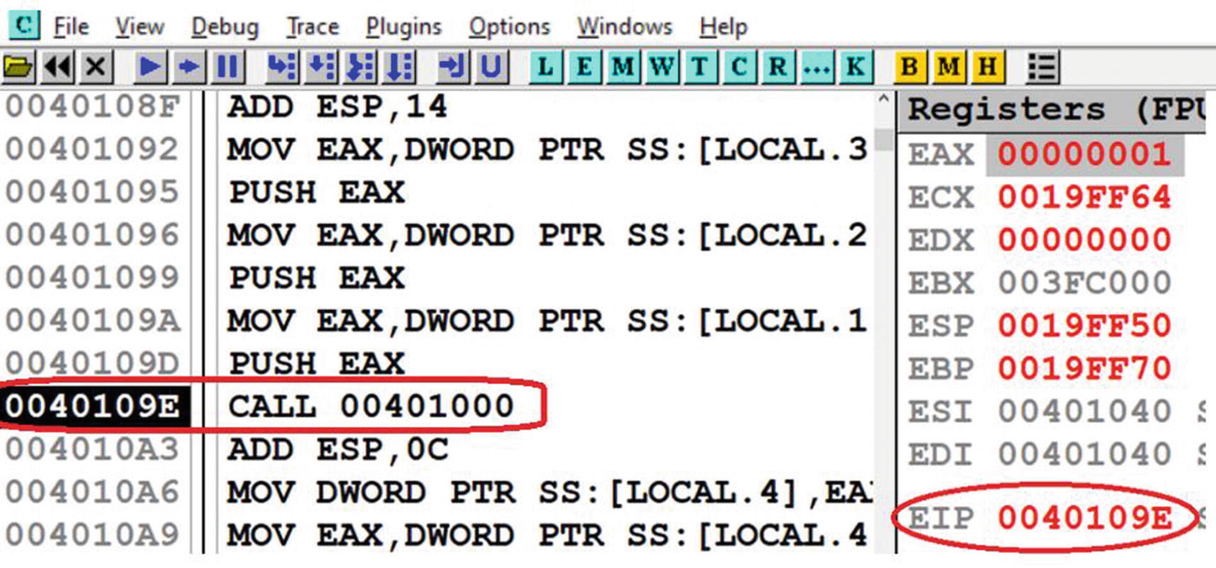
The CALL instruction in Sample-16-1.exe which we step over
Now, if you step over at this instruction, OllyDbg jump straight to 0x4010A3, bypassing the execution of all instructions inside the function call pointed to by the CALL’s target 0x401000.

Result of stepping into the CALL instruction at 0x40109E of Sample-16-1 (also seen in Figure 16-23 )
Run to Cursor
step into and step over execute a single instruction at a time. What if we want to execute the instructions up to a certain instruction without having to step through instructions one by one. You can do this by using the Run to Cursor debugging option, where you can take your cursor to the instruction in the Disassembly window and highlight the instruction by clicking it. You can now press F4 for the Run to Cursor option.
To try this out, restart debugging Sample-16-1.exe by either using the Ctrl+F2 option or the Restart button from Figure 16-21. OllyDbg starts the program and breaks/stops at the starting address 0x401040. Now scroll to the instruction at address 0x40109E, click it, and then press F4. What do you see? The debugger run/execute all the instructions up and until 0x40109E and then stops/breaks. You can also see that the EIP is now set to 0x40109E.
Do note that Run to Cursor does not work for a location that is not in the execution path. It similarly won’t work for a previously executed instruction that no longer fall in the execution path of the program if it continues execution. For example, for our hello world program Sample-16-1.exe, after you have executed till 0x40109E, you cannot Run to Cursor at 0x40901D; that is, the previous instruction unless you restart the debugger.
Run
Run executes the debugger till it encounters a breakpoint (covered later), or the program exits or an exception is encountered. F9 is the shortcut for Run. Alternatively, you can use the button shown in the menu bar, as seen in Figure 16-21. You can also use the Debug Menu option from the menu bar to use the Run option.
Now restart the debugger for Sample-16-1.exe using Ctrl+F2. Once the program stops/breaks at 0x401040, which is the first instruction in the main module, you can now click F9, and the program executes until it reaches its end and terminates. Had you put a breakpoint in the debugger at some instruction or had the process encountered an exception, it has paused execution at those points.
Execute Till Return
Execute Till Return executes all instructions up and until it encounters a RET instruction. You can use this option by using the fast access button the menu bar, as seen in Figure 16-21 or the shortcut key combination of Ctrl+F9.
Execute Till User Code
You need this feature when you are inside a DLL module and want to get out of the DLL into the user compiled code, which is the main module of the program you are debugging. You can use this option by using the fast access button the menu bar, as seen in Figure 16-21 or the shortcut key combination of Alt+F9. If this feature does not work, you need to manually debug till you reach the user compiled code in the main module of the program.
Jump to Address
You can go/jump to a specified address in the program that is being debugged in OllyDbg using Ctrl+G. The address to which you want to jump into can be either an address in the Disassembly window or the Memory window from Figure 16-18. Using the keyboard shortcut prompt you a window which says Enter the expression to follow. You can type in the address you want to jump to and then press Enter to go to the address.
Note that you won’t execute any instructions during this step. It only takes your cursor to the address you input. There won’t be any change in the EIP register or any other register or memory.
As an example, if you have Sample-16-1.exe loaded in OllyDbg, go to the Disassembly window and click Ctrl+G and key in 0x40109E. It automatically takes your cursor to this instruction address and displays instructions around this address. Similarly, if you go to the Memory window and repeat the same process, keying in the same address, it loads the memory contents at this address in the Memory window, which in this case are instruction machine code bytes.
Breakpoint
Breakpoints are features provided by debuggers that allow you to specify pausing/stopping points in the program. Breakpoints give us the luxury to pause the execution of the program at various locations of our choices conditionally or unconditionally and allow us to inspect the state of the process at these points. There are four main kinds of breakpoints: software, conditional, hardware, and memory breakpoints.
A breakpoint against an instruction tells the debugger to pause/stop/break the execution of the process when control reaches that instruction.
You can also place a breakpoint on a memory location/address, which instructs the debugger to pause/stop/break the execution of the process when data (instruction or non-instruction) at that memory location is accessed. Accessed here can be split into either read, written into, or executed operations.
In the next set of sections, let’s check how we can use these breakpoints using OllyDbg. We cover conditional breakpoints later.
Software Breakpoints
Software breakpoints implement the breakpoint without the help of any special hardware but instead relies on modifying the underlying data or the properties of the data on which it wants to apply a breakpoint.

Software breakpoint on an instruction set on Sample-16-1.exe
Now execute the program using F9 or the Run fast access button from Figure 16-21, and you see that the debugger has executed all the instructions up and until the instruction 0x40109E and paused execution at this instruction because you have set a breakpoint at this instruction. To confirm, you can also see that the EIP is now at 0x40109E. This is almost the same as Run to Cursor, but unlike Run to Cursor, you can set a breakpoint once, and it always stops execution of the program whenever execution touches that instruction.
Hardware Breakpoints
One of the drawbacks of software breakpoints is that implementing this functionality modifies the value and properties of the instruction or data location that it intends to break on. This can open these breakpoints to easy scanning-based detection by malware that checks if any of the underlying data has been modified. This makes for easy debugging armoring checks by malware.
Hardware breakpoints counter the drawback by using dedicated hardware registers to implement the breakpoint. They don’t modify either the state, value, or properties of the instruction/data that we want to set a breakpoint on.
From a debugger perspective setting a hardware breakpoint compared to a software breakpoint differs in the method/UI used to set the breakpoint; otherwise, you won’t notice any difference internally on how the breakpoint functionality operates. But do note that software breakpoints can be slower than hardware breakpoints. At the same time, you can only set a limited number of hardware breakpoints because the dedicated hardware registers to implement them are small.

Setting hardware memory breakpoint in for Sample-16-2.exe at 0x402000
In the next section, we talk about memory breakpoints and explore a hands-on exercise on how to set a memory breakpoint using hardware.
Memory Breakpoint
In our previous sections, we explored an exercise that set breakpoints on an instruction. But you can also set a breakpoint on a data at a memory location, where the data may or may not be an instruction. These breakpoints are called memory breakpoints , and they instruct the debugger to break the execution of the process when the data that we set a memory breakpoint has been accessed or executed (depending on the options you set for the memory breakpoint).
From a malware reversing perspective, memory breakpoints can be useful to pinpoint decryption loops that pick up data from an address and write the unpacked/uncompressed data to a location. There are other similarly useful use-cases as well.
You can set a memory breakpoint both in software and hardware. Do note that setting a software memory breakpoint on a memory location relies on modifying the attributes of the underlying pages that contain the memory address on which you want to break. It does this internally by applying the PAGE_GUARD modifier on the page containing the memory you want to set a memory breakpoint on. When any memory address inside that page is now accessed, the system generates STATUS_GUARD_PAGE_VIOLATION exception, which is picked up and handled by OllyDbg.
Alternatively, you can also use hardware breakpoints for memory, but again do remember hardware breakpoints are limited in number. Either way, use memory breakpoints sparingly, especially for software.
Let’s now try our hands on an exercise that sets a hardware memory breakpoint. Let’s get back to Sample-16-2.exe and load it in OllyDbg. In this sample, the encrypted data is located at 0x402000, which is accessed by the instructions in the decryption loop and decrypted and written to another location. Let’s go to the address 0x402000 in the Memory window, by clicking Ctrl+G and enter the address 0x402000. You can then right-click the first byte at address 0x402000 and select Breakpoint ➤ Hardware, which presents you the window, as seen in Figure 16-26. You can select the options; that is, Access and Byte, which tells the debugger to set a hardware breakpoint on the Byte at 0x402000 if the data at that address is accessed (read or written).

Hardware memory breakpoint at 0x402000 of Sample-16-2 shows up in red
Our memory breakpoint set at 0x402000 has been hit, and the process paused

Software memory breakpoint set on an entire memory chunk 0x402000– 0x402045 of Sample-16-2.exe
You can also set both software and hardware breakpoints using IDA. We leave that as an exercise for you to explore in the next section.
Exploring IDA Debugger

While opening a new file for analysis in IDA, it pops up a window asking you to select the format of the file it should be loaded as

Settings for IDA that helps display raw opcode bytes in the Disassembly window

IDA disassembler view after a program has been loaded for analysis
IDA setting to select the debugger to use for starting the debugger

IDA debugger setting to set starting pause point while debugging programs

IDA debugging view made to look similar to the OllyDbg view in Figure 16-18

OllyDbg representation and beautification of variables and args in Sample-16-3
The layout is quite similar to OllyDbg. The same Disassembly window, Register window, Memory window, and Stack window are present in IDA like it did with OllyDbg in Figure 16-18. We closed two other windows—thread window and modules window—that opened on the right and then readjusted their window sizes to arrive at the OllyDbg type look.
Shortcuts in IDA and OllyDbg for Various Functionalities and Their Description
Shortcut | Description |
|---|---|
Ctrl+G for OllyDbgG for IDA | Go to the address location. This does not execute code. |
F7 | Step into a CALL instruction, which executes the call instruction and stops at the first instruction of a called function. |
F8 | Steps over instructions, including CALL instructions. |
F4 | Run to Cursor. Executes the process up until the instruction which you have selected with the cursor. |
F9 | Run the process and executes its instruction until you hit a breakpoint or encounter an exception or the process terminates. |
F2 | Sets software breakpoint in the disassembly. |
Ctrl+F2 | Restart debugging the program |
As an exercise, you can try to debug the samples in IDA like the way we did in OllyDbg in the previous section. Try stepping in/out of instructions. Set breakpoints. IDA Pro is a more complex tool with various features. The power of IDA Pro comes up when you can use all its features. A good resource to use to learn IDA Pro in depth is The IDA Pro Book by Chris Eagle (No Starch Press, 2011), which should come in handy.
Keep the keyboard debugger shortcuts handy, which should allow you to carry out various debugging actions quickly. You can avail of the same options from the debugger menu using the mouse, but that is slower.
Notations in OllyDbg and IDA
Both OllyDbg and IDA disassemble in the same manner, but the way they present us, the disassembled data is slightly different from each other. Both carry out some analysis on the disassembled assembly code and try to beautify the output assembly code, trying to make it more readable to us. The beautification process might involve replacing raw memory addresses and numbers with human-readable names, function names, variable names, and so forth. You can also see automatically generated analysis/comments in the Disassembly window, Stacks window, and Register window in OllyDbg. Sometimes even the view of the actual disassembly is also altered. But sometimes you need to remove all this extra analysis and beautification so that you can see the unadulterated assembly instructions so that you understand what’s happening with the instructions.
Let’s now look at some of these beautification and analysis modifications done by both OllyDbg and IDA Pro and how we can undo them to look at the raw assembly underneath it.
Local Variable and Parameter Names
Both OllyDbg and IDA automatically rename the local variables and parameters for the functions. OllyDbg names the local variables with the LOCAL. prefix, while IDA names the local variables using the var_ prefix. Similarly, in OllyDbg, the arguments passed to the functions are named using the ARG prefix, while in IDA, they are represented using the arg_ prefix.
You can now open Sample-16-3 using OllyDbg and go to the address at 0x401045 using Ctrl+G, which is the start of a function. As you can see in Figure 16-36, OllyDbg has disassembled the machine code at this address, analyzed and beautified the assembly code it generates, renamed the local variables in the function, and the arguments passed to the function to produce the output.

IDA representation and beautification of variables and arguments in Sample-16-3
Compare the generated assembly from both OllyDbg and IDA Pro, see how they vary. Repeat this process for various other pieces of code at other address locations and compare how the analyzed assembly output varies between OllyDbg and IDA.
Now that you know that both tools modify the generated assembly code and beautify them and pepper it with its analysis, let’s now investigate how to undo this analysis.
Undoing Debugger Analysis

Removing OllyDbg’s analysis on the assembly code in Sample-16-3
Instruction at Address 0x401045 in Sample-16-3 After Removing OllyDbg Analysis

Removing IDA’s analysis on the assembly code in Sample-16-3
Instruction at Address 0x401045 in Sample-16-3 After Removing IDA’s Analysis
As you can see, IDA removes the analysis to convert the local variable var_4 as [ebp-4], while OllyDbg from earlier converts LOCAL.1 as DWORD PTR SS:[EBP-4]. Well, both are the same. OllyDbg adds SS, which is the stack segment register. You see in disassembly other segments registers like DS, ES, but let’s not bother about these. Another thing you notice is that OllyDbg adds DWORD PTR, which tells that the variable is a DWORD in size.
As an exercise, undo the analysis at various points in the code and compare the unanalyzed code between OllyDbg and IDA. Extend this exercise to various other samples that you have as well.
Now that we have an understanding of how to use OllyDbg and IDA Pro to both disassemble and debug programs, in the next section, we start exploring various tricks that we can use to identify various high-level language constructs from chunks of assembly code. The ability to identify high-level language code from the assembly easily helps us analyze assembly code and understand its functionality.
Identifying Code Constructs in Assembly
Reverse engineering is the process of deriving human-readable pseudocode from the assembly code generated by disassemblers. We need to recognize variables, their data types, which may be simple data types like integer, character, or complex ones like arrays and structures. Further, we may need to identify loops, branches, function calls, their arguments, and so forth. Helping us identify the higher-level language code constructs helps us speed up the process of understanding the functionality of the malware we are analyzing. Let’s now run through various hands-on exercises that let’s identify these various code constructs.
Identifying The Stack Frame
Every function has its own block of space on the stack called the stack frame that is used by the function to hold the parameters passed to the function, its local variables. The frame also holds other book-keeping data that allows it to clean itself up after the function has finished execution and returns, and set the various registers to point to the earlier stack frame.
A Simple C Code to Demonstrate Stack Frames

Visualization of the stack frames for the sample C code in Listing 16-15, when func_a() calls func_b()
Please note from the figure that though the stack is shown as moving up, the stack always grows from higher address to lower address, So the memory locations at the top have an address that is lower than the ones it.
Each stack frame of a function holds the arguments passed to it by its caller. If you check the code listing, func_a() invokes func_b() passing it two arguments. Passing the arguments is done by the help of the PUSH instruction, which pushes the argument values to the stack. The boundary point on the stack before the arguments are pushed onto the stack defines the start of the called function (i.e., func_b’s stack frame).
The passed arguments are stored on the stack frame as indicated by arg_p and arg_o in the figure.
The return address from the called function func_b back to its caller function func_a is pushed/stored in func_b’s stack frame, as seen in the figure. This is needed so that when func_b() decides to return using the RET instruction, it knows the address of the instruction in func_a() where it should transfer its execution control.
It then sets the EBP to a fixed location on its stack frame. These are called EBP-based stack frames. We discuss them shortly.
Then space is allocated for its two local variables: var_e and var_f.
EBP Based Stack Frames
You have a stack frame present for func_b() while the function is executing, which is referenced by the code inside the function for various purposes, including accessing the arguments passed to it by its caller—arg_o and arg_p—and to access its local variables var_e and var_d. But how does it access these various data inside the stack frame?
The program can use the ESP as a reference point to access the various data inside the stack frame. But as you know, the ESP keeps moving up and down based on whether any PUSH or POP or any other ESP modifying instructions are executed inside the function. This is why EBP pointers are popularly used instead of ESP as a reference point for a stack frame, and access various data locations inside the stack frame. These stack frames are called EBP-based stack frames.
In EBP based stack frames, the EBP pointer is made to point to a fixed location in the currently active running function’s stack frame. With the location of the EBP fixed to a single address in the stack frame, all data access can be made with reference to it. For example, from Figure 16-40, you can see that the arguments are located the EBP in the stack and the local variables the EBP in the stack. Do note that although we said and, the stack grows from higher to lower memory address. So, the address locations the EBP in the figure are higher than the address pointed to by EBP, and the address locations the EBP in the figure are lower than the address pointed to by the EBP.
Now with the EBP set, you can access the arguments passed to the function by using EBP+X and the local variables using EBP-X. Do note these points carefully, because we are going to use these concepts to identify various high-level code constructs later down in the chapter.
Identifying a Function Epilogue and Prologue
Function Prologue Usually Seen at the Start of a Function
The first instruction saves the current/caller_function’s EBP to the stack. At this instruction location, the EBP still points to the stack frame of this function’s caller function. Pushing the EBP of the caller function, lets this function reset the EBP back to the caller’s EBP, when this function returns and transfers control to its caller.
The second instruction sets up the EBP for the current function making it point to the current function’s stack frame.
The third instruction allocates space for local variables needed by the current function.
Now the three instructions form the function prologue, but there can be other combinations of instructions as well. Identifying this sequence of instructions helps us identify the start of functions in assembly code.
Function Epilogue Usually Seen at the Start of a Function
- 1.
The first instruction resets the ESP back to EBP. This address in EBP to which the ESP is assigned points to the address in the stack frame to which the ESP pointed just after the first instruction in the function epilogue, which is the caller function’s EBP.
- 2.
Running the second instruction pops the top of the stack into the EBP, restoring the EBP to point to the caller function’s stack frame.
- 3.
The third instruction pops the saved return address from the stack to the EIP register, so the caller function starts executing from the point after which it had called the current function.
Sometimes you may not see these exact sets of instructions in the function epilogue. Instead, you might see instructions like LEAVE, which instead carries out the operations conducted by multiple of the instructions seen in the function epilogue.
Identifying Local Variables
C Program That Uses Local Vars, Compiled into Sample-16-4.Exe in Samples Repo

Disassembly of Sample-16-4.exe's main() function showing us the local vars
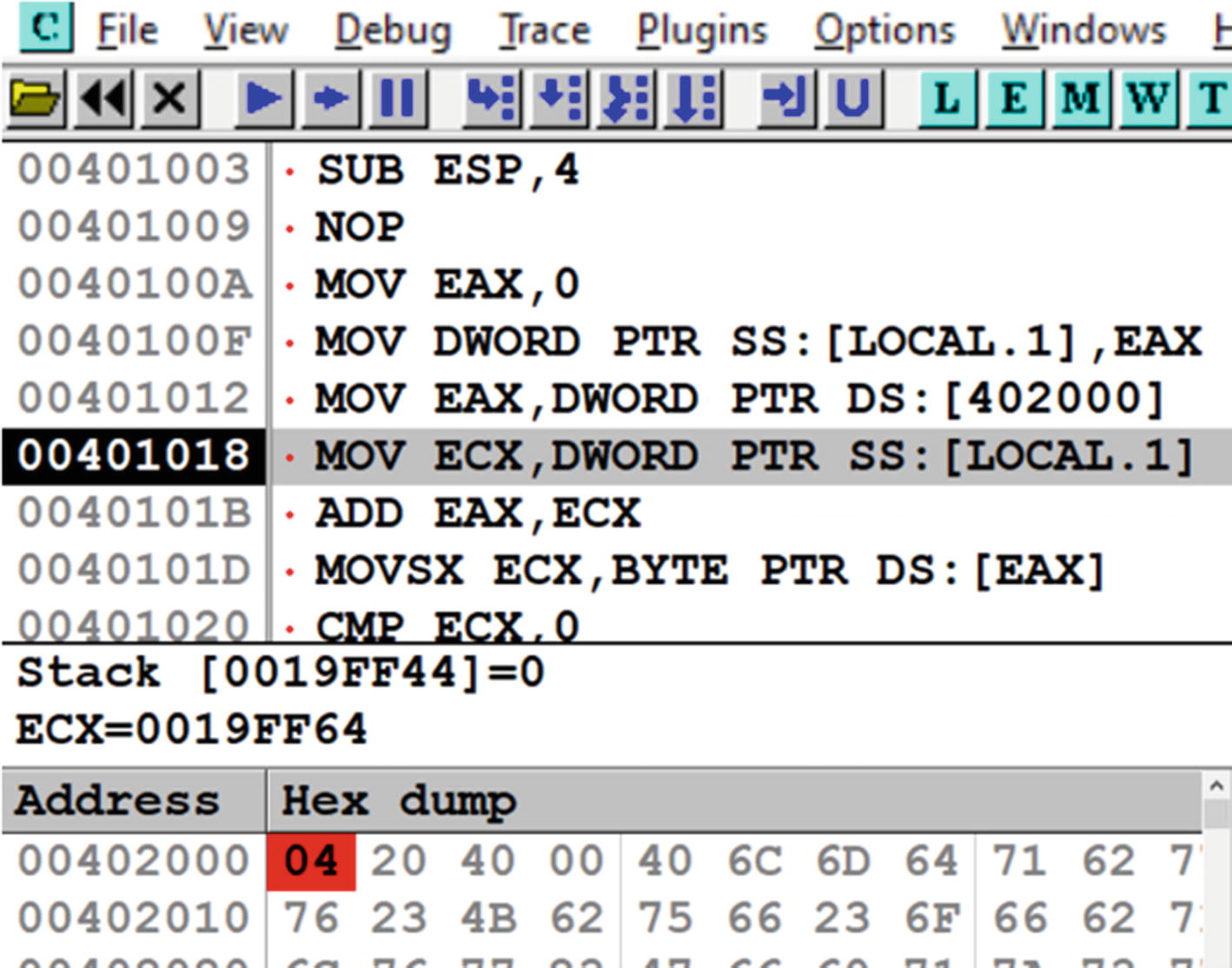
How do you identify the local variables that are part of this function? The easiest way is to let OllyDbg do the work for us. OllyDbg uses the LOCAL. Prefix for all its local variables in a function. There are three local variables: LOCAL.1, LOCAL.2, and LOCAL.3, thereby indicating the presence of three local variables on the stack. Usually, the local variables are accessed using the memory indirect operators’ square brackets [] that also tells us when these variables are being accessed to be read or written into. If you look at the disassembly and map it to our C program in Listing 16-18, LOCAL.1 map to the variable a, LOCAL.2 maps to b and LOCAL.3 maps to c.
Now the method relies on OllyDbg successfully analyzing the sample, but there are various times when OllyDbg analysis fails, and it doesn’t identify the local variables in a function, thereby failing to identify any of the local variables. You no longer have this LOCAL prefix from OllyDbg. How do you identify these local variables then?
You learned earlier that every function has a stack frame, and while a function is being accessed, the EBP pointer is set to point to the currently executing function’s stack frame. Any access to local variables in the currently executing function’s stack frame is always done using the EBP or the ESP as a reference and using an address that is lesser than the EBP; that is, the EBP in the stack frame, which means it looks something like EBP-X.

Actual disassembly for LOCAL.1, LOCAL.2 and LOCAL.3 seen after removing analysis
As you can see, LOCAL.1, LOCAL.3, and LOCAL.2 are referenced using [EBP-4], [EBP-0C], and [EBP-8]. All are references against the EBP pointer, and lesser than the EBP; that is, the EBP in the stack, thereby indicating that the variable at these memory address [EBP-4], [EBP-8] and [EBP-0C] are local variables of the function.

Location of local variables on the stack for the main() function of Sample-16-4.exe
Identifying Pointers
C Program That Uses Function Pointers Compiled into Sample-16-5 in Our Samples Repo

Disassembly of the main() function in Sample-16-5 that shows pointers
Block 1: These two instructions translate to LOCAL.1 = 1, which in C code maps to a = 1.
Block 2: The instruction loads the address of LOCAL.1 into EAX.
Block 3: This translates to LOCAL.2 = EAX, where EAX contains the address of LOCAL.1.
But how do you identify a pointer variable? Now, if you go back to our section on x86 instructions, you know that LEA loads an address into another variable, which in our use case, we are loading the address of a local variable LOCAL.1 into EAX. But then we store this address we have stored in EAX into another local variable LOCAL.2, which all translates to LOCAL.2 = EAX = [LOCAL.1]. Remember from the C programming language that addresses are stored in pointers. Since from the instructions, we finally store an address of LOCAL.1 into LOCAL.2, LOCAL.2 is a local variable that is a pointer.
So, to identify pointers, try to locate address loading instructions like LEA and locate the variables in which the addresses are stored, which should indicate that the variables that store addresses are pointers.
Identifying Global Variables
C Program That Uses a Global Variable Compiled into Sample-16-6.Exe in Our Samples Repo

Disassembly of the main() function in Sample-16-6 that shows global vars
Block 1: The instruction moves the content at address 0x402000 into EAX.
Block 2: This instruction translates to LOCAL.1 = EAX, which indicates that we are assigning a local variable with the value of EAX.
To be honest, OllyDbg does all the hard work for us. OllyDbg names all the local variables with the LOCAL.* naming scheme and the global variables with pretty much the DS:[<address>] naming scheme, revealing to us that DS:[402000] must be a global variable.
OllyDbg names all local variables using the LOCAL. naming scheme. But it didn’t name DS:[402000] with a LOCAL. prefix naming scheme, which means it is not a local variable.
Now you know that local variables are located on the stack, which means DS:[402000] isn’t located on the stack. Anything that is not on the stack is global.
We exploited the hard work put in by OllyDbg analysis to figure out the presence of a global variable. But there’s another manual way to figure this out as well. Just click the instruction that accesses the LOCAL.1 variable, and the Information Display window show you the address of this variable as 0x19FF44 (please note that address might be different on your system). In the Information Display window, it also says that this address is on the stack, so your job is done, but let’s figure this out the hard and long way. We also have the address of the other variable as 0x402000.

The Memory map window shown by OllyDbg for Sample-16-6 that clearly shows the memory blocks used by the stack that hold the local variables
If you go back to our earlier chapters, this memory map window looks very similar to the view of memory in Process Hacker. If you notice the OllyDbg tags, it clearly states the various memory blocks that represent the stack, indicating which is the stack and the other memory blocks. If you compare the two addresses we obtained earlier, 0x19FF44 and 0x402000, we can easily figure out by their locations in the memory blocks, that one is located on the stack and the in one of the other segments like the data segment (i.e., global).
Identifying Array on Stack
Sample C Program Using Arrays Compiled into Sample-16-7 in Our Samples Repo

Disassembly of the main() function in Sample-16-7 that shows the array being indexed in the loop, like in the C program

Representation of the arrays in the stack memory from running Sample-16-7
At the disassembly level, an array may not be identified when they are initialized, and each element looks like a regular data type–like integer. Arrays can only be identified when the elements in the array are getting accessed. To identify the presence of an array, identify if the elements of an array are accessed using an offset or index against a single element or reference point in memory.
Let’s look back to the disassembly at the instruction at 0x41218B in Figure 16-47. Let’s look at the second operand of the instruction, which is [ECX*4+EBP-14] where EBP-14 is the address of the first element of the source array. Trace back the value stored in ECX to the instruction at 0x412188, which is the value of the local variable [EBP-34]. At each iteration of the loop, the value of this index [EBP-34] is incremented by 1. But if you come back to the instruction at 0x41218B, we use this index value from ECX (i.e., from EBF-34) in every single iteration, but always against the same local variable at EBP-14. The only constant here is the local variable EBP-14, with the variance being ECX ([EBP-34]), thereby indicating that the constant reference variable EBP-34 is an array index variable.
the Iterations of the Loop from the Assembly Loop in Figure 16-47
If you refer to the image, the operand accesses the first element of the array in the first iteration and second element in the second iteration and the third one in the third iteration. If you refer to the instruction in 0x41218F in Figure 16-47, you find the same pattern, but instead, elements are being written into the destination array at EBP-28, the same way the source array is accessed earlier.
Identifying Structures on Stack
C Program That Uses a Structure Var on the Stack Compiled into Sample-16-8 in Our Samples Repo

Disassembly of main() in Sample-16-8 showing our structure var being accessed
The amount of space allocated for a structure is by adding up the elements of the structure, including padding.
In assembly code, the elements of a structure are accessed in most cases by using the topmost member of a structure as a reference point/member/index. The address of the rest of the elements in the structure is done by adding offsets against this base reference member of the structure.
Now in the figure, LOCAL.3 is a local variable as identified by OllyDbg, and this local variable corresponds to the variable s1 inside main(). So to identify a structure in the assembly code, identify if multiple other assembly instructions are accessing data locations on the stack by using a single variable as a reference point.
Checkout instruction 0x40100F in Block (1), and you see that it assigns a value of 1 to LOCAL.3 local variable. At this point, it looks like LOCAL.3 is a simple data type. Hang on!
Now instructions in Block 2 again loads the address of the same LOCAL.3 variable into EAX but then tweaks this address by 4 bytes against this LOCAL.3 address. It is a clear indication that it is accessing another variable at [LOCAL.3] + 4. A clear indication that it is using the address of LOCAL.3 data variable as a reference point.
Next, checkout instructions in Block 3. It again loads the address of the same LOCAL.3 variable into EAX, but this time it tweaks the address by 8 bytes against this LOCAL.3 address. It is a clear indication that it is accessing another variable at [LOCAL.3] + 8. Another clear indication that the LOCAL.3 data variable is used as a reference point.
The Block (2) and Block (3) addresses are composed and accessed by all of them using the address of LOCAL.3 as a reference index address, all indicating that LOCAL.3 is some kind of complex data structure variable, like a structure or a union and the various other addresses composed/referenced off it are its members.
To figure out the size of the member variables, you need to figure out the size of the data access from the instructions. In the assembly case, the various data members are assigned values considering DWORD as the size; hence the members are 4 bytes in size. Now you might point out that the second data member char c is a character and hence should be only 1 byte in size. This is where padding comes in. A compiler pads the extra 3 bytes in the structure for various purposes, including efficiency, giving you the illusion in the assembly that the variable is 4 bytes in size.
Function Call Parameter Identification
C program Compiled into Sample-16-9, to Illustrate Function Args Identification
How the parameters are passed on to the sum() function
How the sum() function accesses these parameters passed to it

Parameters passed from main() to sum() in the main() function of Sample-16-9 corresponding to its C code in Listing 16-24
If we map the instruction back to our C code LOCAL.1 maps to variable a and LOCAL.2 maps to variable b. These variables are passed as parameters to the sum() function. The instruction at 0x401022 calls the function sum() using its address 0x401036. Parameters are passed to the sum() function by pushing them to the stack. But if you notice the order, the second parameter is pushed first, followed by the first parameter. You can execute step by step till the call instruction 0x401022 and see the location of the parameters on the stack.
Now, if we step into the sum() function using the F7 keyboard shortcut, you notice that the address of the instruction right after the call instruction at 0x401022; that is, 0x401027 is pushed to the stack. This address is the return address from the sum() function back to the main() function, after sum() has finished execution.

The sum() function in Sample-16-9 that shows the parameters passed to it
OllyDbg has again analyzed this function for us. Identifying the arguments passed to the function is made super easy by OllyDbg as it has done all the analysis and hard work. It has represented the first parameter passed to it with ARG.1 and the second with ARG.2. It has also identified the total from the C code in Listing 16-24 as LOCAL.1. But the LOCAL.1 here is local to this sum() function, and is different from LOCAL.1 in the main() we saw in Figure 16-50. Job done!
But let’s try to figure this out the hard way, just in case OllyDbg fails to analyze the code. The EBP is used as a reference point in the currently executing function's stack frame, and any references to its local variables and arguments passed to it are accessed using the EBP. The arguments passed to the function are placed in the stack below the EBP of the function’s stack frame, which means it can be accessed using EBP+X. Though we said it is below the EBP, we still referenced it using + X. The reason is though the stack moves up, it moves from a higher memory address range to a lower. So, the EBP is at a lower address than its arguments placed below it on the stack, which is at a higher address range.

Identifying arguments passed to functions using EBP, as seen for the two instructions in Sample-16-9 for which we removed analysis
Identifying Branch Conditions
Conditions are the steering factors for the flow of execution in programs. In high-level languages, if/else, switches, and so forth, are constructs that test for conditions and alter the execution flow to different branches based on the outcome of their tests. In assembly, you are not going to see these. Instead, the test for conditions are carried out by instructions like CMP, ADD, and SUB and based on the results of the test instructions, which update various status flags in the flags register, various conditional JUMP instructions like jnz, jns, and so forth, branch and alter the execution flow to various points in the code.
Simple C Program That Uses Conditional Branching Which We Have Compiled into Sample-16-10 in Our Samples Repo

Disassembly of the main() function in Sample-16-10 that shows conditional checks and jumps
It is very easy to identify the presence of conditional branch instructions. All you need is to look for some sort of comparison instruction and then a branch instruction that tests for conditions in the flags register. We see both instructions here. One is the CMP in Block 2, which does the comparison. The other is the subsequent JNE in Block 4, which branches to different portions of the code based on the test results of the previous CMP, which then update the flags register. The two blocks of code that map to the if and the else branches can be identified in Block 5 and Block 6.
Using OllyDbg, we had to manually figure out the various branches and blocks, but IDA Pro makes it easy to identify branch instructions using its graph view. IDA has two modes to view disassembly: the text view and the graph view. The text view is the linear view, like how OllyDbg shows, while the graph view displays the code in the form of flowcharts. You can switch between the views by right-clicking disassembling and choosing the right view.
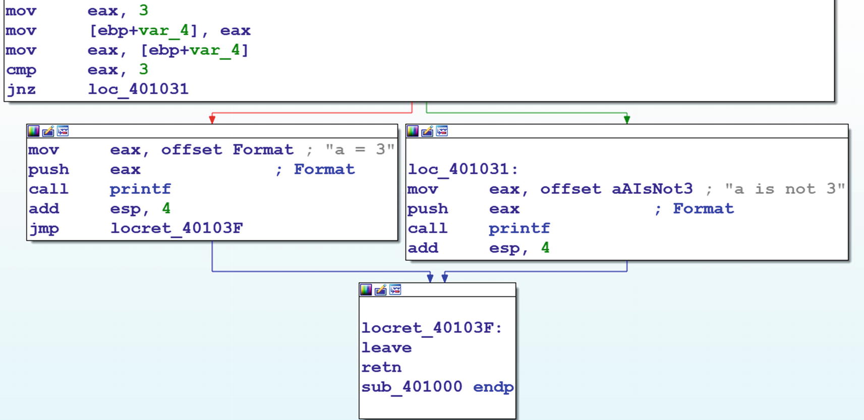
Conditions branching shown very clearly using IDA’s graph view
Identifying Loops
Every programming language uses loops with the help of for and while constructs. Malware makes use of loops for various reasons—iterating through processes, files, or other objects, encrypting or decrypting data, even to implement a pseudo sleep, and so forth. Hence it is important for malware analysts to look out for loops in disassembly code since they might point to some kind of special functionality used by the malware.
Loops in assembly language are identified by a backward jump in the execution flow; that is, the target of the jump is a lower address compared to the instruction making the jump. The jump should be a near jump; that is, not to another memory block or segment. The jump can be either conditional or unconditional. Also, loops are not meant to run forever. So there has to be a condition for exiting the loop. If a LOOP instruction creates a loop, then the value of ECX determines the exit condition. In other cases, exit conditions are determined by the presence of instructions like CMP and conditional jump instructions like JNZ, JNE, and so forth. So to identify loops, look for a combination of some kind of immediate short backward jump and some kind of comparison and conditional jump instructions.
C Program Using While Loop Compiled into Sample-16-11 in Our Samples Repo

Disassembly of main() Function of Sample-16-11.exe which clearly shows the presence of a loop through OllyDbg’s analysis that shows a backward jump
As you can see in the figure, you see a short backward jump at 0x401029 to 0x401012. You then see a comparison instruction at 0x401015, and then immediately, the next instruction at 0x401018 is a conditional jump instruction JG. The body of the loop can be identified by the address of the instruction where the unconditional backward jump-starts and the address of the backward jump instruction itself. Loop identified!
Now there is another easier way to identify loops, and that is allowing OllyDbg to analyze the sample. As you can see in the figure, OllyDbg shows you the loop and its body using the arrow line connecting the unconditional jump instruction at 0x401029, and the jump target 0x401012, which we have pointed out in the figure. Job done!

IDA identifying and displaying loops in graph view for Sample-16-11
There are more complex loops where there are loops inside loops. Sometimes the number of iterations in the loop can be quite high, and debugging each item may be frustrating. You can run past the entire loop by setting a breakpoint on the exits of the loop. Also, there might be several conditions and comparisons in the body of a loop to exit the loop.
In our sample from Figure 16-55, you can exit the loop at 0x40102B, as indicated by the JG 0x40102B conditional jump instruction earlier at address 0x401018. You should similarly locate all the exit points in a loop and set breakpoints on all of them if you are not interested in iterating through the loop while debugging it and want to exit it early.
Making Disassembly Readable
OllyDbg, IDA as well as other debuggers are armed with features that can be helpful to read disassembly. The tools have coloring features that can display different categories of instructions in different colors. Some of the features and plugins can convert the linear view of code into flowcharts, which makes it easier to figure out loops and branches. Other features include automatic analysis and commenting. Let’s explore some of the features in this section.
Color Coding
Different kinds of color coding schemes are provided by various disassemblers to make the code more readable. In OllyDbg, you can right-click any of the Windows and scroll down to Appearance under which you can select Colors or Highlighting. For example, under the Highlighting menu, you can choose the Christmas tree coloring scheme, which is our personal favorite. Similarly, with IDA, you can go to Options ➤ Colors to select various coloring and appearance options for instructions, variables, and other assembly constructs.
Labels and Comments
Both IDA and OllyDbg have options to label or name an address. When another instruction in the code references that address you previously labeled, the label that you used for that address open in the Information window.
Having the ability to label addresses of the start of the functions or the address of certain code blocks with specific names is a great way for you to tag certain code blocks based on functionality. For example, when you are analyzing malware code that implements decryption or encryption functionality inside a function of its, you can label the start address of that function with your own name, like EncryptionFunction or DecryptionFunction. Now when you click any other instruction in the program that references these function addresses, you see the label names that you gave these function addresses earlier in the Information window.

Adding a label to instruction addresses in OllyDbg

Adding a label to instruction addresses in IDA
IDA and OllyDbg also both provide options to comment on instructions in the Disassembly window, which gets saved by the debugger so that next time you reanalyze the same sample, you can look at the comments you added at various instructions.

Adding comments to instructions in OllyDbg
Tracking Variables

Tracking a variable in IDA
Accelerating Disassembly Analysis
Reverse engineering is about converting assembly language to high-level language pseudocode. Reading millions of lines of assembly code in malware is not going to be easy. We need to find out techniques that can help us to go through assembly code faster. Choosing what to read and what not is important. Smartly using features of the disassembler and debugger can help us to locate useful code. In this section, we introduce various other tricks that you can use to quickly analyze assembly code and understand its functionality.
Skipping Compiler Stub and Library Code
You have noticed that we have asked you to go to the main() function in all the examples we demonstrated till now and not the entry point of the PE file. Do you know why we did that? Isn’t the entry point the start of the main() function? When we compile a program, the compiler inserts some code of its own. This code is present in the entry point of the executable and goes all the way to the main() function, which has been written by the programmer. This code is called the compiler stub.
The code in the compiler stub varies from compiler to compiler and even between versions of the same compiler. The compiler stub is present in any executable, whether benign or malware, as long as it’s been generated from a compiler. It’s a waste of time to look at the compiler code since it is present in both benign and malware executables.
Compiler stubs can have specific patterns, and the main function can also be located by parsing the compiler stub. IDA’s FLIRT signatures are there for your help. They can take you across the compiler stub when you open an executable in IDA, thereby helping you get past this unwanted compiler code and into the true functionality of the sample you are analyzing, saving precious time.
Condensing Instructions With Algebra
We saw many of the instructions like MOV, ADD, SUB, INC in assembly, and all these can be represented with arithmetic equations. For example, MOV EAX,9 can be represented as EAX=EAX+9. Similarly, INC EAX can be translated to EAX=EAX+1.
Sample Assembly Code from Sample-16-2 That We Now Analyze
the Assembly in Listing 16-27 Simplified into Simple Algebraic Equations
Now this one boils down to an arithmetic equation. If we further solve the equation, this reduces to EAX=004020F0 + LOCAL.1. So translations help us simplify a complex set of instructions into simpler algebraic equations. Once you have translated the, you can add it as a comment so that you can refer the comment back if you were to pass through the same instructions later while debugging the code. This is especially useful if you are analyzing decryption and obfuscation loops in malware that involve multiple instructions that involve various arithmetic instructions that modify data.
Using Decompilers
Disassembly is a process of converting the raw machine code bytes into a more readable assembly language. But assembly language is not as easy to read as high-level languages like C, Java, and so forth. But we can use a process called decompilation , which can convert the machine code back to high-level language code (which is even better for reverser engineers).
There are various tools that can decompile code (Hex-Rays decompiler, Sandman decompiler, Cutter, Ghidra, x64Dbg) that integrate the Sandman decompiler into its UI. x64Dbg is another great debugger that looks and works just like OllyDbg, and the integration of the Sandman decompiler into its UI makes it even better. The best part of it all is that it’s free!

The decompile C code for the main() from Sample-16-2, the original C code for which is seen in Listing 16-29
Source Code for main() of Sample-16-2
Blocks and Flowcharts
It is extremely hard to read a large piece of Disassembly Code and figure out what it’s doing. No assembly code executes linearly. There are branches taken, calls made, all of which break the linear execution flow. A better way to view the disassembly instructions and understand its execution flow is to use a debugger graph view.
IDA Pro tool provides this graph view feature, which analyzes the assembly code and breaks it into multiple blocks and presents it into a graph view, showing the various execution flows across these blocks. IDA Pro figures out the start and end of the blocks based on various conditions like branches from the jump and call instructions, execution transfer to an instruction from another remote instruction that is not the instruction linearly behind it. Apart from IDA Pro, other debuggers also provide graph view, including OllyDbg using a plugin called OllyGraph, but none of them are as fancy as the IDA Pro one.

List of Function in the Function window

IDA graph view for the main() function of Sample-16-2
IDA has broken up the main() function of Sample-16-2.exe into seven blocks. It also shows the control execution flow among these blocks. This is much easier to read and understand and figure out the various branches taken by the instructions in the function than if you were to read the same assembly instructions for this function if it is displayed linearly.
References (XREF)
References or XREF is a feature provided by disassemblers that given a piece of code, instruction, data, the debugger point to other locations in the code that references that piece of code. For example, you have a function call, and as you know, every function call starts at an address. Using references, you can figure out all the other locations/instructions in the code that references that function address. Another example is you have a piece of data in the code, say a global variable, which has an address. Using references, you can figure out all the other locations/instructions in the code that references that global variable’s address.
Let’s take a hands-on exercise to show references in action. For our exercise, please take Sample-16-12 from the samples repo, which is a GandCrab malware sample. Now start by loading this sample in BinText to list all the strings in this sample. You can verify from the strings listed that one of the strings in the sample is -DECRYPT.txt.

The Setup strings window shown by IDA that helps you set up various string display options

IDA String window displaying strings in the Sample-16-12
As seen, we have checked all the options and set the minimum length of string to be displayed as three. That should give us good visibility into all the strings in the sample. With that set, the strings are seen in Figure 16-65.
You can see the string -DECRYPT.txt that we were also able to locate previously using BinText. Let’s try to analyze this particular string, which most probably is related to the ransomware's ransom note.
References to the string we earlier double-clicked in Figure 16-65
As seen in the screenshot, IDA says that the string has been referenced at the offset 9F from the start of function at 0x4074B9, which in the end translates to 0x4074B9 + 0x9F, which is 0x407558. If you click the XREF, as seen in the figure, it takes you to the address 0x407558 located inside function 0x4074B9, where this string is referenced.

Call chain in Sample-16-12 that shows the code flow that finally ends up referencing the DECRYPT-txt string located at 0x41A0D8
As you can see in the figure, -DECRYPT.txt is referenced by code inside the function that starts at 0x4074B9, which in turn is called by another function that starts at 0x407949, which in turn has been called by another function at address 0x407BD3 and so on.
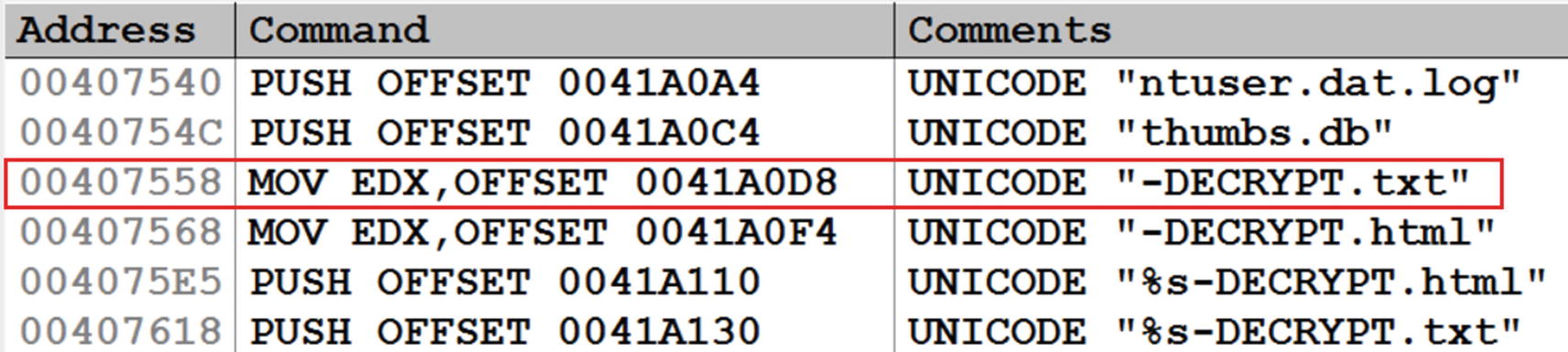
Viewing all the strings for Sample-16-12 in OllyDbg
The first column is the address where the string has been referred, which is 0x407558, which is what we discovered in IDA.
Do note that if you have not disabled ASLR as per the requirements of the analysis VM setup we discussed in Chapter 2, these addresses we are showing might vary while you open it on your VM.

Instruction/Code XRefs in IDA
IDA is saying that this function has been referenced at offset 0x85 inside another function located at 0x407949, which all added up is address 0x4079CE. Since this is a reference to code, it is called CODE XREF by IDA, as seen in the figure. Similar to how you built the XREF graph for data earlier, you can right-click the start of the function and select Xref graphs to to display the graph view of how the execution flows to this function.
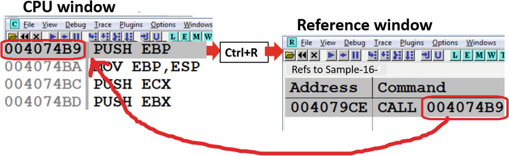
References to code instructions shown by OllyDbg for the function 0x4074B9 in Sample-16-12
As seen in the image, the instruction at 0x4074B9 has been referenced from the instruction at 0x4079CE.
References to API calls
Malware uses Win32 APIs extensively to carry out their malicious intentions like injecting code into other processes, stealing information, connecting over the network, and so forth. Our APIMiner tool could figure out what APIs are used during execution. But from a reverse engineering point of view, these Win32 APIs are called from somewhere within the malware code/functions. Using XREF, you can also figure the code blocks or functions which invoke various Win32 APIs used by the sample.

The imports of Sample-16-12, as shown by IDA Pro in its Imports window.

References to CreateFileW API calls by the code in Sample-16-12 shown by IDA
As you can see in the figure, it shows multiple locations in the malware’s sample code where CreateFileW is invoked: sub_401261 + 40, sub_40303E + DE, and so on. If you want to see the graph for the XREF, you can right-click the API name CreateFileW and choose Xrefs graph to, just like we did for strings.

References to CreateFileW API calls by the code in Sample-16-12 shown by Olly
Advance Usage of Debuggers
Debuggers can do a lot more than disassemble and debug a program. Let’s go through some other advanced use-cases of debuggers that should help us with various other tasks that come in handy while reversing malware.
Observing API Calls and Parameters
While debugging malware, you are going to encounter a lot of Win32 APIs that are used by them. While either analyzing or reversing malware, it is important to know the various arguments passed to these Win32 APIs and to figure out the values returned by them, since this tells us more about the functionality and state of the malware. In our analysis chapters, we could obtain both the result returned, and the parameters passed using APIMiner.
Similarly, with debuggers, including OllyDbg, you can also obtain the same information. As an exercise, check out Sample-16-13 using OllyDbg and go to the instruction located at address 0x411A8E call VirtualAlloc API.

API parameters on stack passed to VirtualAlloc API call by Sample-16-13
Now when it comes to figuring out the output or return value of the Win32 API, you need to step over the CALL instruction so that EIP is at the next instruction after the CALL instruction. In this case, the return value of VirtualAlloc, which is the address allocated by it, is placed in the EAX register.
Do note that different APIs return the output in different locations. Some might return output in memory locations that are passed as parameters to the stack. Some might use registers. Some other kinds of results are stored in memory buffers, which you must inspect in the Memory window.
Breaking on Win32 APIs
When reversing, analysts often prefer to skip part of malware code and look at what’s interesting to us. For example, if you want to analyze the network activity of malware, you can skip analyzing/reversing the rest of the malware code and instead set a breakpoint on the Network Win32 APIs like HttpSendRequest(), Send(), Recv().
If you execute the program after setting the breakpoints at APIS, the debugger stop/pause execution when these APIs are finally involved by some malware code. You can then find out the part of the malware code which has invoked the API and then can further analyze that specific piece of malware code.
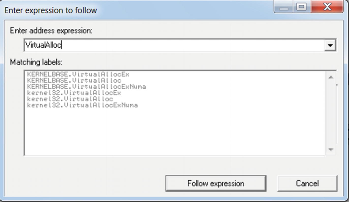
Use in OllyDbg Ctrl+G to list various VirtualAlloc APIs reference by Sample-16-13
While entering the API name, you get suggestions which you can select, which in our case here it is KERNELBASE.VirtualAlloc, which is the second option in Figure 16-75. Alternatively, you can press enter on any of the options shown, which take you to the location of the API in the corresponding DLL, where you can manually set a breakpoint by using F2.

The breakpoint on kerne32.VirtualAlloc which we set earlier on Sample-16-13 is now hit
VirtualAlloc internally calls VirtualAllocEx API . The breakpoint breaks at the first instruction at the start of the API call (i.e., prologue). If you execute until the end of the API call (that is, the RET instruction at address 0xDCE7A18), you see the results of the API, which are stored in the EAX register.

After we run Execute till user code, after hitting the breakpoint, we arrive at the next instruction in the main sample code that invoked the VirtualAlloc API
Conditional Breakpoints
Do note that there are a lot of calls to a single Win32 API in a sample. If we simply put a breakpoint at a Win32 API, we break at all the instances of that API, and every time we have to go back to the main sample code to figure out the functionality of the malware code that involved the API and why it invoked the API. Sometimes the malware code might not invoke the Win32 API directly, but via some other Win32 API only if there was a way to break on an API only when it met certain conditions. In comes the conditional breakpoint feature in debuggers.
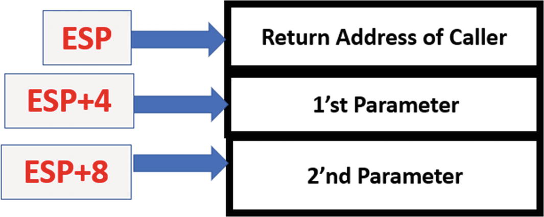
The state of the stack right at the first instruction of the VirtualAlloc API call

The conditional breakpoint on VirtualAlloc API for Sample-16-13 that only breaks if the Size parameter passed to it is 0x1000
Conditional breakpoints like are very useful to discard the unimportant API calls and only break on execution if it meets certain more specific conditions. Conditional breakpoints should be used in combination with Dynamic Analysis tools like APIMiner, which we can run right before we can use a debugger to reverse a sample. Using APIMiner lets you know the various Win32 APIs and the number of times those APIs are called and the various arguments that are passed to it. Armed with this knowledge, you can specify conditional breakpoints based on the various argument values used by the sample we next want to debug.
Debugger Events
Spawning a child process
Creating/terminating a new/existing thread
Loading/unloading a module/DLL
Debuggers provide us the option to pause the execution of the process we are debugging at various process events, pretty much like a breakpoint, thereby allowing us to catch these events and analyze the state of a program. This feature is very useful while analyzing malware because most malware, as you learned in Chapter 10, spawns child processes and new threads for various activities like Code Injection and Process Hollowing.

Events pane of OllyDbg’s options where we can set the behavior for handling of various events seen by OllyDbg
IDA also has similar options as OllyDbg provides, via the Debugger ➤ Debugger Options in the menu, as seen in Figure 16-34.
Patching
A lot of times, malware may refuse to execute on your machine because of some armoring features. For example, if the malware discovers that it is being debugged or analyzed, it might exit early. But with the help of debuggers, we can view all the instructions and functions that implement these armoring checks. Better yet, with the help of debuggers, we can patch/modify the instructions, code, and registers live as the process is executing, thereby allowing us to bypass running these armoring checks.
As an example, check out this Sample C program seen in Listing 16-25, which we have compiled into Sample-16-10. As you can see in the C code, the if branch is always taken, since a is initialized to 3 at the start of the program. Let’s see if we can patch this code dynamically at runtime to make it take the else branch.
Load Sample-16-10 in OllyDbg and set a breakpoint at the instruction at address 0x401018, which is the instruction that decides to either jump into the if branch or else branch, as seen in Figure 16-53.
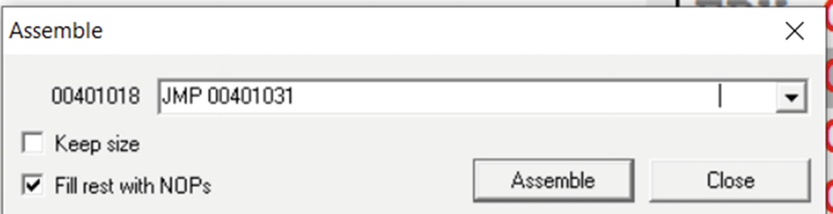
Patching JMP instruction in OllyDbg at address 0x4010108 of Sample-16-10

After patching the instruction at 0x401018, the disassembly looks like

Executing Sample-16-17 after patching its instruction at 0x401018 into an unconditional jump instruction
Using the patching feature, we not only can modify the instruction code, but also the data contents in memory, the values of various registers, the values of flags register, the return values from Win32 APIs—all of it per our needs.
Call Stack
You saw that setting a breakpoint at a certain location and then executing the code executes the entire code until the breakpoint. Often it might be required for us to know what other functions are executed in between in the call up to our breakpoint instruction/function.
Sample C Program That Makes Use of Nested Function Calls
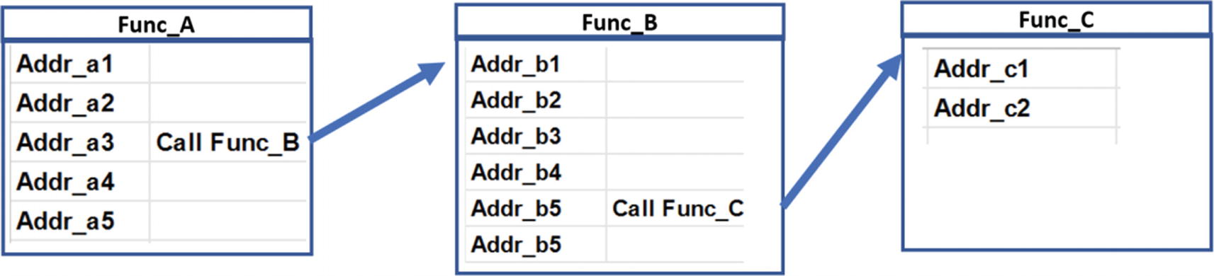
Illustration of the flow of control across the various functions in Sample-16-14
The C code has been compiled into Sample-16-14, which you can then load using OllyDbg. Once loaded, set a breakpoint at the start of func_c(), which is the address 0x401067, post which you can run the program by pressing F9, which should then break/stop execution at func_c() where we have set our breakpoint.
Now a call stack is a feature of the debugger that shows the entire chain of function calls that has led to the current instruction getting executed. Now since we have hit the breakpoint inside function func_c, we are currently paused inside func_c right at the first instruction of this function.
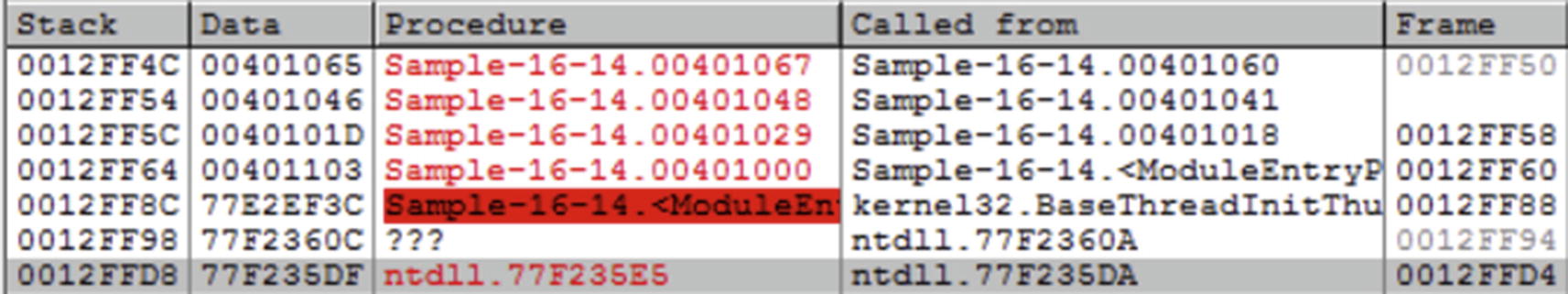
Call stack window in OllyDbg shown after we hit the breakpoint we set on func_C for Sample-16-14
Summary
Dynamic analysis and static analysis are super-fast ways to analyze and classify a sample. But sometimes they may not be enough for various reasons, including the presence of armoring in the samples we are analyzing and also for the need to dissect deeper into a sample to write better detection. In comes the process of reverse engineering to dive deeper into samples and debug them.
In this chapter, you learned what reverse engineering means and the various processes involved in reversing a sample. We started by learning the basics of the x86 Instruction format and run through various important sets of instructions that we encounter while reversing malware samples. We then explored what debuggers mean and how to use them using OllyDbg and IDA as our reference debugger examples.
Using debuggers, we then did various exercises in which you learned how to identify high-level code constructs in the assembly code. Identifying high-level code constructs in the assembly code helps us speed up the analysis of the assembly code while reversing samples.
You also learned various other additional features debuggers to better present the assembly code and explore ways to tag the assembly code for our future reference. Finally, you learned various other advanced debugging tricks, including using XREFs and patching assembly code that are part of useful tricks reverse engineers use to reverse malware samples.