5 | Signal Characteristics
When building and testing electronic circuits it can be very useful to gauge the performance of a particular design by sending test signals through the circuit and performing measurements on the resulting output waveform. The simplest measurements take the form of a single number, perhaps showing the average voltage level or the frequency of the signal under examination. More elaborate measurements may be presented in graphical form.
Time Domain and Frequency Domain Representations
When it comes to visualising the information in a signal, two primary formats exist as illustrated in Figure 5.1. A time domain representation of a signal (Figure 5.1a) shows how the signal’s amplitude changes over time. This would directly correspond to the variations observed in the voltage level which constitutes an audio signal propagating inside a circuit.

Figure 5.1 An audio signal can be viewed either in the time domain (a), or in the frequency domain (b). These two types of visualisation both represent the same signal, just highlighting different aspects.
The second form (Figure 5.1b), designated a frequency domain representation or frequency spectrum, shows a snapshot of the signal at one point in time. A short snippet of the signal is analysed and broken up into all the individual frequency components which are present at that moment. The amount of energy at each frequency is represented by the height of the line at that position along the X axis of the graph. This representation shows more explicit detail than the time domain view, but only represents one single instant in time.
A real time analysis or RTA view of a signal shows each of these levels dancing up and down as the signal changes over time. This kind of view is commonly found in audio analysis software packages as well as in many digital oscilloscopes. The visual-isation will often be simplified by breaking it down into (most commonly either ten or thirty-one) bands, each one representing a range of frequencies as shown in Figure 5.2.
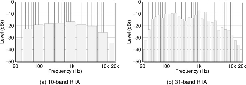
Figure 5.2 A real time analysis (RTA) view might break the audio band up into any number of frequency sub-bands. Ten bands and thirty-one bands are the two most common types of RTA display. These are also commonly called one octave and one third octave displays respectively because each band covers that approximate bandwidth.
Typical audio is a complex signal made up of many constantly varying components at different frequencies, as illustrated in Figure 5.1. As such it is often more instructive to use simpler test signals when performing tests. In order to get the most out of such test procedures it is important to have a good understanding of the nature and characteristics of the standard test signals encountered, and the terms and analytical tools used to describe their various aspects and behaviours.
Signals can be modified in a number of standard ways. The most important of these (phase shift, polarity inversion, rectification, clipping, and crossover distortion) are described next. Following this the commonest test signal types are examined, starting with the most fundamental signal component, the sine wave. After that the related wave shapes of square, triangle, ramp, and sawtooth are briefly examined.
Having looked at signals and their representations in both the time and frequency domains, and considered the commonest types of signal distortion encountered, the final section in this chapter introduces the decibel, and examines the relationship between linear and logarithmic representations of the same data. Decibels are encountered everywhere in audio technology and in electronics in general. They represent a powerful method for measuring and comparing the levels or amplitudes of different signals.
Phase and Polarity
Phase refers to the relative position in time of two signals or two components within a signal. It is useful to remember that while polarity talks about top to bottom changes (amplitude), phase talks about left to right changes (time). For a sine wave a phase shift of 180° looks identical to a polarity flip, but the same is not the case for an arbitrary waveform. These concepts are illustrated in Figure 5.3.

Figure 5.3 Phase and polarity illustrated in the case of a sine wave and an audio signal. If the time shifted audio signal were mixed back in with the original audio signal, comb filtering would result. Each frequency component would experience a different degree of phase shift and so a different level of reinforcement or cancellation, depending on each component’s frequency (or more directly its associated wavelength).
While polarity is a binary function (flipped or not flipped) referring to the relationship between the top half and the bottom half of the signal, phase is a continuous function (any number of possible states) referring to the relative position of two signals or signal components in time.
A static phase relationship specifically applies to sine waves of the same frequency and it is not on the whole meaningful to talk about the relative phase of two more complex signals. Two arbitrary signals will constantly move in and out of phase with one another. When both are up at the same time or both are down at the same time they might be considered in phase, and when one is up as the other is down they can be said to be, to a greater or lesser extent, out of phase. This is not however a very useful analysis on the whole. Two sine waves of the same frequency will have a constant phase relationship, being either completely in phase or some specific degree out of phase. Phase is measured in degrees with 360° in a full cycle. If two sine waves of the same frequency are moved relative to each other they will continually move in and out of phase. Phase relationships become very important when multiple signals (be they acoustical or electrical) are being combined or otherwise manipulated. Comb filtering and other unwanted artifacts can result. Some electronic circuits are also capable of altering the phase relationships of various components of a signal. Sometimes this is an unwanted side effect (as in filters and EQs) and sometimes it is used to advantage (as in effects like phasers and flangers).
Unlike phase, polarity is a binary concept. That is to say there are two possible states of polarity, which are often referred to as positive and negative. That portion of a signal which lies above the midline is said to have positive polarity while the portion below the midline is said to have negative polarity. One very common function available on mixing desks and some other audio equipment is a polarity invert or polarity flip function. This process takes the incoming signal and flips it over so that the positive half becomes negative and the negative half becomes positive. This very simple and very useful function is often (but erroneously) referred to as ‘phase invert’ instead of the correct name of ‘polarity invert’.
Rectification
Rectification refers to the removal or reversal of the negative half of any signal, such that no part of the resulting signal extends below the midline. The two basic forms of rectification, called half wave rectification and full wave rectification are illustrated in Figure 5.4. Half wave rectification is when the portion of the signal below the line is set to zero. Full wave rectification is when the portion of the signal below the line is folded back up above the line.
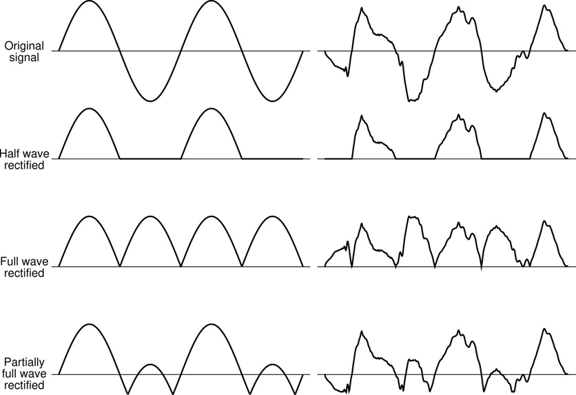
Figure 5.4 Examples of half wave and full wave rectification as applied to a sine wave and an arbitrary signal.
Rectification is a common process in electronics. Indeed another name for a diode is a rectifier because this is pretty much exactly what a diode does. One diode on its own easily achieves half wave rectification while full wave rectification is simply implemented using four diodes in a configuration called a bridge rectifier. The details and applications of these circuits are fully addressed in Chapter 16 on diodes. Rectification is often utilised in distortion and octave up effects due to the nature of the harmonic distortion this kind of processing adds to a signal. It is also a key stage in the operation of a standard linear power supply, converting an AC signal into a DC one. This application is examined in Chapter 16.
Clipping
Clipping is closely related to rectification and is often also implemented using diode based circuitry. Basic symmetrical hard clipping as shown in the second waveform in Figure 5.5 is among the most common (and certainly one of the simplest) approaches used to implement audio distortion as seen in myriad classic guitar effects pedals.
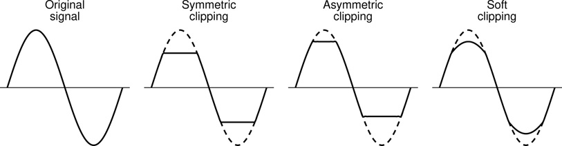
Figure 5.5 Various types of signal clipping. The dotted lines show the shape of the unclipped signal in each case for comparison.
The idea is simply that some portion of the signal peaks are reduced or removed completely. Half wave rectification could be seen as an extreme form of asymmetrical clipping but in general clipping will be applied somewhat more gently. Even a small amount of clipping (only removing the very tips of the largest signal peaks and troughs) can result in a highly distorted sound. As illustrated in the third and fourth waveforms in Figure 5.5 two common variations on the theme exist. Asymmetrical clipping is where one side of the signal waveform is clipped more heavily than the other, which introduces a different balance of odd and even harmonics, and thus a different character to the sound. The idea in soft clipping is that rather than simply lopping off the tops and bottoms of the waveform they are instead rolled off more gently, producing less high frequency harmonics in particular and thus resulting in a somewhat less harsh form of distortion.
Clearly there is much scope for experimentation here. Different amounts of asymmetry and varying degrees of hard/soft balance in the clipping introduced will result in a broad palette of possible sounds. Again, these possibilities are more fully explored in the chapter on diodes, as well as in some of the project work presented in the final part of the book.
Crossover Distortion
Closely related to the distortion introduced into a signal due to clipping is the concept of crossover distortion, as illustrated in Figure 5.6. This is when, rather than modifying or removing the positive and negative peaks of a signal as in clipping, it is instead altered at the point where it crosses the midline. This is referred to as crossover distortion.
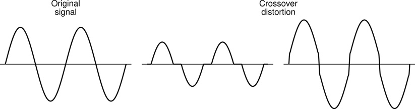
Figure 5.6 Crossover distortion can manifest in a number of different ways.
Crossover distortion can take many varying forms, depending on the mechanism generating it. The two extremes shown in Figure 5.6 illustrate either end of the spectrum, but various other kinds of steps and deformations are possible. This kind of signal modification is less commonly utilised in distortion effects (although by no means unheard of). On the other hand, it is a problem commonly encountered in amplification circuits which use some form of symmetrical circuit architecture to perform amplification of the positive and negative portions of a signal. If the circuit is not correctly designed and appropriately configured or calibrated, then crossover distortion can be introduced at the point where the signal amplification task is handed over from one side of the circuit to the other. This most often takes a form close to the first of the two variants shown.
The Sine Wave
The sine wave is the simplest of all possible signals. As illustrated in Figure 5.7b all the energy in such a signal is concentrated at a single frequency. This makes measurement and comparison of sine wave signals very easy to perform. As such it is an effective test signal to use when building and experimenting with audio circuits.

Figure 5.7 In the case of a sine wave all of the signal’s energy is concentrated at a single frequency. Hence the familiar time domain wave shape in (a) corresponds to a single line in the frequency domain (b).
In Figure 5.8 some of the key characteristics of a sine wave are shown. In the horizontal or X direction, which can represent either time (period) or distance (wave-length), the main metric is the length of one cycle. For an electrical signal travelling in a circuit this will be measured as a time (perhaps one millisecond per cycle). This is called the waveform’s period and is usually represented by the lowercase Greek letter tau (τ).
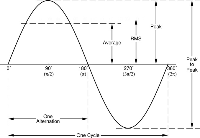
Figure 5.8 Measurements on a sine wave. The labels in brackets along the X axis (π/2 etc.) show the equivalent angles measured in radians rather than degrees.a
Distance measures may arise more frequently when considering an acoustic sound wave travelling through the air, in which case the quantity measured would be the waveform’s wavelength, typically represented by the lowercase Greek letter lambda (λ). In the case of an acoustic rather than an electrical signal it is often of more interest to know the wavelength, although a measure of the period can be useful in acoustics also.
Frequency and wavelength are related to each other by the speed of propagation of the signal (whether acoustic or electrical). For acoustic signals the speed in question is the speed of sound (about 340m/s). Electrical signals are a form of electromagnetic energy. Electromagnetic energy in a vacuum propagates at the speed of light, about 3 × 10⁸m/s (after all light is electromagnetic radiation). In a wire, electricity propagates at a considerable fraction of this speed; still very fast indeed.
The actual speed can vary considerably depending on various characteristics of the wire or cable in question. In both the acoustic and electrical cases the relationship between speed (c), wavelength (λ), and frequency (f) is defined by Eq. 5.1. So audio electrical signals, with frequencies in the range 20Hz–20kHz, have very long wavelengths. As such it can be seen that the wavelengths of electrical signals in general only become comparable (and therefore significant) for very long cables (e.g. telephone lines or cable TV) or very high frequencies (such as in digital systems).
In the context of electronics however the period is the measurement of interest and thus that remains the focus here. The period has units of seconds per cycle, and so for instance the period of the sine wave shown in Figure 5.7 can readily be decerned from the time domain graph as being four milliseconds per cycle. The ‘per cycle’ portion of the unit is commonly omitted when quoting the period of a waveform, and so the period in this case might be reported as four milliseconds or simply 4ms. The implicit ‘per cycle’ should not be forgotten completely as it can be useful when recalling the relationship between period and frequency as discussed below.
_______________________________
A figure more familiar to most than the period of a signal would be its frequency. It is however often the period which is directly available through measurement and so it can be useful to remember that there is a very straightforward relationship between these two quantities: period is one over frequency, and frequency is one over period.
An examination of the units of these two quantities quickly confirms this relationship. Frequency has units of cycles per second (cps), also known as hertz (Hz), while as observed earlier period has the opposite units of seconds per cycle. As such the simple reciprocal relationship between these two quantities should come as no surprise. In electronics it is often easier to measure the period of a signal (for instance with an oscilloscope), but it is often more useful to know its frequency, and so this relationship is very important and often used.
In the vertical, Y direction on Figure 5.8 four amplitude metrics are marked: peak, peak-to-peak, average, and RMS. The peak and peak-to-peak values should be fairly self explanatory. They simply represent the maximum excursion of the signal up from the centreline, and from top to bottom of the waveform respectively. For a sine wave the peak-to-peak measurement is exactly twice the peak value. This is not necessarily the case for more complex signals, which may often be asymmetrical above and below the centreline.
Strictly speaking, the average value of a sine wave is zero, since the waveform is symmetrical around the centre or zero line. What has been marked as ‘average’ on Figure 5.8 might more accurately be described as the half-wave average or rectified average, where the portion of the signal below the zero line is reflected up to lie above it (see later in this chapter for a discussion of signal rectification). Here it could most simply be characterised as the average signal level as measured between 0° and 180° (or indeed 0° and 90°, which would yield the same result due to the symmetry of the waveform). This rectified average level is a simple thing to measure for an electrical signal, requiring only a straightforward circuit in order to perform the task. Unfortunately, its ease of measurement notwithstanding, it is a far less useful metric than the final one marked on the graph, the RMS or root mean square.
The RMS is the value required in all calculations and equations which allow electrical circuits to be analysed and their behaviour predicted. The reasons why this is the required measurement relate to the amount of electrical power in the signal, but is not further addressed here. The name RMS itself is entirely self explanatory, it is calculated by taking the root of the mean of the square. In other words first square the signal, then calculate the mean (or average) of this, and finally take the square root of this calculated mean. It is a simple enough process to describe but not nearly so simple to actually implement when making an electrical measurement.
There are however simple mathematical relationships which connect the peak, average, and RMS levels of a sine wave. Note that these relationships apply only to sine waves and do not extend to arbitrary signals. Eq. 5.3 states that the average is about six tenths of the peak level, while Eq. 5.4 shows the RMS as about seven tenths of the peak. These first two can easily be combined to arrive at Eq. 5.5, which gives the relationship between the sine wave’s average and RMS levels.
This final multiplication factor of approximately 1.11 is often used to convert a measured average voltage value into an estimate of the RMS level of a signal. As previously stated this conversion will be accurate if the signal being investigated is a sine wave, but a significant error can result for waveforms of other shapes. This point is expanded upon in the next section. It is worth noting here that inexpensive voltmeters usually measure the average signal level (which is an easy thing to do), and then scale the result before reporting, in order to approximate an RMS reading. More advanced volt-meters will often carry the moniker ‘True RMS’ to indicate that they implement a more complex design in order to directly measure the RMS signal level rather than estimating it based on a more straightforward average measurement.
Complex Signals
All signals no matter how rich and complex can be decomposed into and analysed as a collection of sine waves of different frequencies, amplitudes, and relative phase relationships as illustrated in the frequency domain plot in Figure 5.1b. By mixing together sine waves at frequencies all along the X axis, with amplitudes given by the height of the plot at each location, the original signal could be reconstituted. Decomposing a complex signal into its constituent sine wave components is a powerful tool for analysis and manipulation much utilised in digital audio systems.
Sine waves provide a simplicity which facilitates easy of analysis but this same simplicity also imposes limitations on their usefulness in testing and characterising the behaviour of audio electronic circuits. The real world audio signals which these circuits will encounter once deployed have a far more rich and complex character. In order to best understand how such circuits will respond and react test signals which more closely resemble true audio might be of some benefit. However the inherent complexity of a regular audio signal renders detailed analysis using such signals difficult or impossible.
For these reasons various test signals of intermediate complexity are often employed when performing test and measurement procedures, more complex than sine waves but simple enough to allow for meaningful observations and measurements to be made. The commonest of these are the square wave, the triangle wave, and the ramp and sawtooth waves.
Square, Triangle, Ramp, and Sawtooth Waves
Each of these waveforms is composed of simple mathematical combinations of a series of sine waves. The specific spectral makeup of these wave shapes is described widely throughout the literature, and can be of particular interest in the design and use of subtractive synthesisers and related circuits. These details are not of immediate concern here and so are left for now. Figure 5.9 gives as much of an overview of the makeup of these signal shapes as is required in the context of this book.

Figure 5.9 Square, triangle, and sawtooth waves in the time and frequency domains. Square and triangle waves are composed of the same frequency components, just in different proportions. The sawtooth involves twice as many frequencies, but in similar proportions to the square wave. The associated ramp wave shape is just a polarity flipped sawtooth, and as such has the same spectral makeup.
It is worth noting the corresponding relationships between peak, average, and RMS levels for these wave shapes, and comparing them to the relationships previously given for the sine wave. In the case of a square wave the relationships are extremely simple and fairly easy to deduce by looking at the shape of the square wave graph. All three values are in fact equal.
In the case of the triangle, ramp, and sawtooth waves things are a little more complicated, but the answers come out the same for all three wave shapes. This is not all that surprising as the three shapes are very closely related, as can be seen both from their time domain and their frequency domain representations, as illustrated in Figure 5.9.
The mathematics behind these relationships is quite straightforward, although it does require some basic calculus. There is no need to get into these details. For those who may be interested, the treatment is presented in the highlighted Box 5.2.
As mentioned in the previous section, while the RMS level is what is usually wanted, the rectified average is easier to measure. Many multimeters therefore measure this and use it to estimate the RMS value. The estimation, which makes an assumption that the signal being measured exhibits sine wave characteristics, can result in a significant error in the reported value. The highlighted Box 5.3 shows how to calculate the errors which will ensue when measuring the standard wave shapes.
Decibels
Decibels are a large and complicated topic, however an in-depth treatment can be sidestepped here. Instead some useful rules and guidelines are provided without getting into the more technical and mathematical background needed to fully explore the subject. For a more comprehensive examination of the use of decibels in audio technology and electronics see for instance Brixen (2011). In the current section just the details needed to understand and usefully employ decibels in the context of this book are presented.
When the size of an electronic signal is measured directly the result will most often be expressed in volts. Audio signals might typically range in size from tens of micro-volts (at the noise floor), up to perhaps some hundreds of volts (for the output of a high powered amplifier). These extremes would correspond to a factor of about ten million between the smallest and largest signals which might be encountered. Using these voltage values directly when measuring, comparing, and visualising audio signals presents two particular issues: the range of numbers employed becomes unwieldy and the values encountered do not relate well to how the ear perceives the loudness of sounds. Using decibels however the same range can be covered by just 140dB.
Thus decibels provide an alternative way of expressing levels and level changes in audio signals that addresses these two difficulties effectively. The primary goal is to provide a system where the unit of measurement relates naturally to the perceived changes in loudness or level of the signal. To achieve this a mathematical function called the log or logarithm is employed (a graph of the log function is given in Figure 5.10). A deep understanding of the properties and behaviour of this function is not required. For the most part it is sufficient to know which button to press on a calculator in order to apply the operation. Some familiarity with the broad shape of the function is however helpful in gaining an appreciation of how decibels behave.
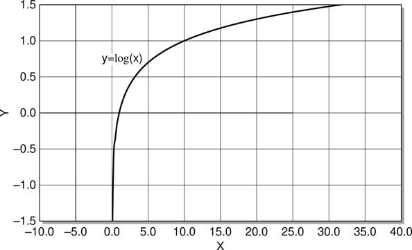
Figure 5.10 Graph of the function y = log(x), which is used to calculate decibel values.
The most pressing difficulty with using voltage values directly when measuring a signal is that the same voltage change in a signal level (say a one volt change) does not correspond to the same change in the perceived loudness for different signals. Changing a quiet signal by one volt will have a dramatic effect, while the same one volt change in a loud signal could go virtually unnoticed. On the other hand, a change of say three decibels in each of the two aforementioned signals will result in very similar changes in the perceived levels of the signals.
A small change in a small signal and a big change in a big signal are required in order to result in the same perceived change in the loudness of the two signals. Therefore a measurement scheme which reflects this nonlinear relationship will make for a more useful and user friendly way of talking about levels and level changes. Returning to the graph in Figure 5.10 helps us to understand how the decibel achieves this goal. The voltage level of the signal can be thought of as being plotted horizontally along the X axis while the decibel values range up and down on the Y axis. Now consider the two cases mentioned previously.
A small signal sits on that part of the graph close to the origin where the line moves up and down very quickly with just small movements left and right. Thus in this region of the graph a small voltage change (along the X axis) will correspond to a relatively large decibel change on the Y axis.
Conversely, a large signal sits farther to the right, on the part of the graph where it takes a large left-right movement to achieve even a small up-down change. Thus for a larger starting signal, a larger voltage change is required in order to achieve the same given decibel change in the signal level. This is exactly the behaviour which is required in order to give values which correspond well to the way in which the human ear registers changes in loudness.
The general equation used for calculating decibel values from raw voltages is given in Eq. 5.6. As can be seen from the equation, two voltages (here called V1 and V2) are involved in any decibel calculation – decibels represent ratios or differences.
All the examples given in the rest of this section should be entered into a calculator as they are encountered, in order both to confirm the answers shown and to gain familiarity with entering such calculations correctly. There are a few different ways in which modern scientific calculators work. It is well worth confirming and solidifying familiarity with a number of different devices.
As an example consider two voltages, V1 = 20 volts and V2 = 10 volts. Inserting these two values into Eq. 5.6 gives:
and so it can be seen that the difference between twenty volts and ten volts is six decibels or, put another way, twenty volts is six decibels larger than ten volts. It is also very useful to remember that if V1 and V2 are swapped the calculated decibel value simply switches sign; in this case the six decibels becomes minus six decibels. This makes sense since if twenty volts is six decibels larger than ten volts then ten volts is going to be six decibels smaller than twenty volts, i.e. −6dB.
Eq. 5.6 allows the decibel relationship between any two voltage levels to be calculated. It does not however in this form provide any method for specifying actual signal levels (entering one volt and two volts into the equation also results in an answer of 6dB, i.e. two volts is six decibels larger than one volt, just as twenty volts is six decibels larger than ten volts). This is useful for comparing levels or specifying changes in level – ‘Signal A is 12dB louder than signal B.’ or ‘Turn track two down by 8dB.’ – but it does not provide a method for indicating what the levels are.
In order to be able to specify an actual voltage level in decibels (‘Set the main volume to X.’), it is necessary to first define a reference level or zero point. This will be the voltage which corresponds to zero decibels on the scale. The use of a standard reference level is indicated by adding a suffix to the decibel unit. There are a number of common reference levels which might be encountered. Two in particular are very commonly found in audio work. Where an uppercase V is added to the units, as in dBV, the reference level is taken to be one volt, i.e. 0dBV = 1.0V. If a lowercase u is encountered (dBu), the zero point is defined to be 0dBu = 0.775V. It does not really matter where these reference levels originally came from but it is useful to remember them.
In order to convert Eq. 5.6 for calculations of dBu or dBV all that is required is to replace the V2 by the appropriate reference level/zero level.
This provides the tools needed to quote signal levels in decibels, in addition to signal level changes, as already explained. It is important to remember that pure decibels (dB) refer to level changes while modified decibels (dBu, dBV, etc.) correspond to actual signal levels. Thus a signal’s level might be changed by +6dB or −12dB, whereas the level might be equal to +4dBu or −10dBV. These two particular levels (+4dBu and −10dBV) are encountered often. They are two signal levels commonly used when designing audio equipment. In order to calculate the voltage levels which they correspond to, Eq. 5.6 needs to be inverted so that instead of entering two voltages to get a decibel value, one voltage and a decibel value are entered in order to yield a voltage. This inverse function is shown in Eq. 5.9.
Returning to the first example and reversing it, this equation provides an answer to the question, what voltage is six decibels smaller than twenty volts?
This calculation confirms the expected operation of the inverse function, returning the original value for V2 from the earlier example. Similarly it is now possible to calculate the signal voltage levels which correspond to the commonly used −10dBV and +4dBu levels mentioned above. Recall that V2 is the reference voltage level for the particular decibel variant used. So for dBV, V2 = 1.0V while for dBu, V2 = 0.775V.
Notice that (as illustrated in Figure 5.10) the logarithm of one is zero (log(1) = 0) so if V1 = V2 then V1/V2 = 1, and dB equals zero. This corresponds to the statement that any level is exactly 0dB different from itself.
In addition to dBu and dBV it is worth being aware of one other modified decibel type commonly encountered. dBr stands for decibels relative, and is often seen used in measurement results and most especially on graphs. It means that the decibels in question have been measured relative to some arbitrary zero level which should then usually be specified.
Two common ways in which these units are used are to show an output level relative to an input level, or to show measurement levels at various frequencies relative to the measurement at 1kHz. In the first case what is being said is that whatever input level is sent into a circuit, the output will be this much different. The second example is used to show the frequency response of a circuit; with a response of 0dB at 1kHz, it shows how many dB up or down the response is at any other frequency. The graphs in Figure 5.1 and Figure 5.2 include axes labelled in dBr indicating that the signal levels are measured relative to an unspecified maximum level. Notice that the values are all negative in these examples, indicating that all the recorded levels are smaller than the maximum possible level by the numbers of decibels shown.
Example Calculation
Returning to the graphs of Figure 5.7, it proves an instructive exercise to confirm mathematically that the two plots do indeed represent the same sine wave in both their frequencies and their amplitudes.
Eq. 5.2 states that frequency is one over period. The period (time for one cycle) can quickly be determined from the graph in Figure 5.7a as being 4mS = 4/1000Sec. Therefore in accordance with Eq. 5.2 the frequency of the time domain sine wave shown in Figure 5.7a must be 1000/4 = 250Hz. Correspondingly the frequency peak shown in Figure 5.7b sits neatly between the 200Hz and 300Hz grid lines indicating a consistent frequency representation between the two graphs.
Turning to the amplitude of the sine wave in question the decibel equations just introduced allow for comparison of this property across the two graphs. In Figure 5.7a the sine wave’s peak level reaches approximately 12V. It is important to remember that decibel levels correspond to volts RMS and so first this peak voltage must be converted to an RMS voltage. As the signal under consideration is a sine wave, Eq. 5.4 can be used to perform the conversion.
It is then a simple matter to convert this RMS value into a level in dBu using Eq.5.7.
Again returning to the plot in Figure 5.7b the frequency peak can be seen to rise just above the 20dBu grid line confirming that the represented amplitudes are also consistent between the two plots.
Linear and Logarithmic Scales
It can be instructive to consider the four possible variations which can arise in graphs with respect to the use of linear and logarithmic scales for the X and Y axes. The four variations depend on whether each axis is plotted with a linear or logarithmic scale. Figure 5.11 shows the same three functions plotted using each of these four variations. (In this case the three functions are actually those for the impedance versus frequency of three fundamental components, which are examined in detail in later chapters. These graphs are encountered again in context at that point.)
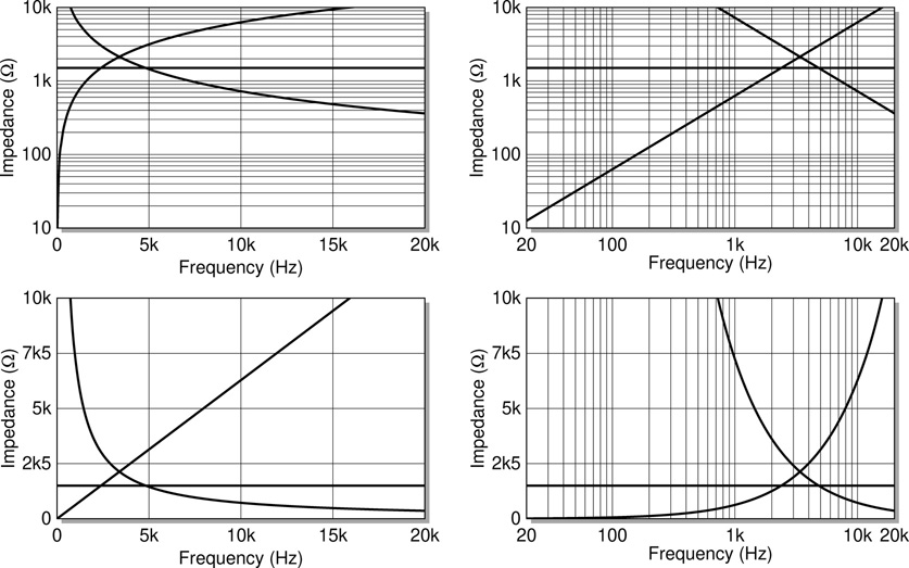
Figure 5.11 Comparison of linear and logarithmic scales.
At least three of these combinations are commonly encountered in the literature on capacitors and inductors and each variant has its place. In general terms the approach using logarithmic scales on both axes is probably most often likely to be the best option in this context. All things else being equal, straight lines are to be preferred as they are easier to interpret and easier to extrapolate. Additionally human perception generally operates in logarithmic terms and so log scales make sense from this point of view also. The frequency steps between musical notes proceed logarithmically as do steps of equal loudness (decibels) and of course the E-series preferred values used to define component sizes also proceed in a logarithmic fashion. As such it often makes most sense to use logarithmic scales to plot such quantities.
However a logarithmic scale can never include zero and so if behaviour at the origin is to be displayed explicitly on a graph then linear scales are necessary. For instance the fact that an inductor’s impedance (theoretically) reaches zero ohms at a signal frequency of zero hertz becomes obvious from a graph using linear scales for impedance and frequency whereas with logarithmic scales this can not be shown. The important thing is to appreciate that both methods of plotting values are encountered regularly, and to gain a sufficient understanding of them and their relationship in order to make best use of the graphical information being presented.
And finally always recall that a scale labelled in decibels is logarithmic by default. The labelling is linear because the linear to logarithmic transformation has already been applied. The underlying quantity (most often voltage in the case of the present work) is transformed from a linear to a logarithmic scale in the calculation which converts voltages into decibels as for instance is used in the frequency domain plots in Figure 5.1, Figure 5.2, and Figure 5.7 at the beginning of this chapter. Thus these graphs are displaying their data using logarithmic scales on both axes despite initial appearances. The two time domain plots in the same figures are by contrast linear in both axes.
It is unsurprising that logarithmic relationships appear so naturally in so many places. Fundamentally they reflect the fact that small changes in small things and big changes in big things result in similar perceived amounts of subjective change.
References
G. Ballou, editor. Handbook for Sound Engineers. Focal Press, 4th edition, 2008.
E. Brixen. Audio Metering: Measurements, Standards and Practice. Focal Press, 2nd edition, 2011.
S. Gelfand. Hearing: An Introduction to Psychological and Physiological Acoustics. Informa Healthcare, 5th edition, 2010.
M. Mandal and A. Asif. Continuous and Discrete Time Signals and Systems. Cambridge University Press, 2007.
B. Metzler. Audio Measurement Handbook. Audio Precision, 2nd edition, 2005.
M. Russ. Sound Synthesis and Sampling. Focal Press, 2nd edition, 2004.
W. Sethares. Tuning, Timbre, Spectrum, Scale. Springer, 2nd edition, 2005.
F. Stremler. Introduction to Communication Systems. Addison Wesley, 3rd edition, 1990.