8 | Electronics Lab Equipment
A few key pieces of equipment allow for a wide range of circuit test and measurement tasks to be accomplished with ease. A good level of familiarity with the equipment available to you can make a huge difference to the success and the enjoyment of audio circuit building. The basic tools of the trade come in a wide variety of shapes, sizes, and price points, but for the most part, while bells and whistles vary widely, the primary functionality provided is consistent and quickly mastered.
Make a new folder on your computer beside the one called ‘Data Sheets’ from Chapter 6, and label it ‘Manuals’. Whenever a new piece of gear crosses your path, find and save the user manual and any other useful documentation you come across. Your equipment will differ from the kit presented in the examples here, but the basics will remain the same. Once you can identify the primary controls and connections, it should not prove difficult to transfer that knowledge to a new piece of equipment of the same type. Four key tools are highlighted, with others mentioned more briefly.
Bench PSUs, or bench power supply units, provide the power for circuits as they are developed and tested. Most of the circuits considered here can be powered from a standard 9V battery or a (non-adjustable) power brick, but the bench PSU provides more flexibility and a number of other advantages.
Function generators produce test signals ideal for injecting into circuits in order to see how they perform under various conditions. By using a carefully controlled input signal rather than an audio track for testing, the performance characteristics of the circuit in question can be much more easily and much more precisely assessed.
Multimeters of various types and form factors allow for basic measurements of voltage, current, resistance, and continuity. They also usually provide for the simple testing of components like diodes and bipolar transistors, and some can incorporate an impressive array of additional functionality.
Oscilloscopes allow the user to visualise and characterise audio and other signals as they pass through circuits under test. They can provide for more detailed analysis than is possible with a basic multimeter.
Audio analysers and advanced test gear such as electronic loads, spectrum analysers, and distortion meters can be very useful in more advanced work, but are beyond the scope of what is needed for the basic tasks considered here.
Software tools covering a wide range of tasks and applications exist. Programs to help in the design of both circuits themselves and circuit board layouts can be a valuable aid. Software interfaces to test and measurement hardware also exist. The softscope is a particularly common application; a software interface providing oscilloscope functionality via an audio sound card or similar hardware frontend.
Workbench tools in general are a given, and will not be considered further here. Accumulate all you can lay your hands on: wire cutters and strippers, pliers, screwdrivers, clamps, magnifiers, assorted sprays and fluids, glues and lubricants, blades, hacksaws, drills and rotary tools, safety goggles, socket sets, spanners, files... The list is endless. A well stocked (and well organised) workbench makes the conduct of any job a much more straightforward affair.
Soldering and desoldering, and the associated tools are addressed separately in Chapter 10 – Constructing Circuits.
Bench Power Supply Units
The term bench PSU is used to refer to an adjustable power supply designed to provide versatile DC powering options on the workbench, as opposed to a standard PSU, which is designed to be supplied with or incorporated into a specific piece of equipment and provide just those power signals which are needed for that particular task.
AC outputs are possible from a PSU (bench or standard) but in the current context are much less generally useful and less commonly encountered than the standard DC supply. The variable autotransformer or variac® is the most common format for a variable AC power supply. A variable autotransformer allows for the AC voltage to be dialled up to any desired level, often including levels beyond the mains input level (remember transformers can step up as well as stepping down). These devices are often used for slowly ramping up to full mains voltage when servicing or fixing a piece of mains powered equipment such as a power amplifier. They are extremely useful in this application, but are not the kind of PSU which is of general interest here.
A typical bench PSU (Figure 8.1) will usually be able to provide a DC output voltage level between zero and some maximum, at a current up to some maximum level. Adjustment of the voltage, and often also the current limit, is possible through the frontend controls, with displays providing feedback as to the voltage and current levels during configuration and in operation.
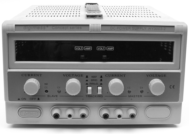
Figure 8.1 HY3003-2 dual linear DC power supply (0–30V DC, 3A per channel).
If the maximum current level is reached the device may switch from constant voltage mode into constant current mode. These two modes are often indicated by two LEDs on the front panel labelled CV (for constant voltage) and CC (for constant current). Normally it is the aim to operate in constant voltage mode, but if the load attached to the PSU is too heavy, and the current limit is reached, then the PSU will reduce the voltage level to whatever is needed in order to allow no more than the set maximum current to flow. This is constant current mode. By setting a maximum current just a little higher than the current which a circuit is expected to draw, it is possible to minimise the chances of damaged or destroyed components and equipment due to an error or a fault in the circuit being powered.
It can be useful to consider the operation of the device under four general headings: inputs, outputs, controls, and displays.
Inputs
A bench PSU almost always derives its power via a mains power connection. Advanced models can include remote control interfaces for automated operation but this is less common and not considered here. No other inputs are required.
Outputs
Terminals or connection points are provided in order to deliver power into the circuit. They are usually colour coded – black for negative and red for positive. Often a separate ground point is provided, typically coloured green or black and marked with an earth ground symbol ![]() . This ground terminal will be hardwired directly to the earth of the mains power lead.
. This ground terminal will be hardwired directly to the earth of the mains power lead.
The positive and negative outputs can either be floating or referenced to ground. The outputs on the devices in Figure 8.1 and Figure 8.2 are floating by default. The middle terminal in each cluster of three is the earth ground mentioned above, and can be connected to either positive or negative if specific ground referencing is desired (a jumper can be seen in Figure 8.2 bridging between the negative and ground terminals; this can be rotated to connect the positive rail to ground instead, if desired). The two outputs on the supply in Figure 8.1 are designed so that they can be wired in series to make a split or dual power supply if needed. A split supply provides three connection points: positive, negative, and ground.

Figure 8.2 Trio PR-602A linear DC power supply (0–25V DC, 3A), with two presets and one freely variable output control.
Two supplies with their negatives hardwired to earth ground can not be wired in this way or one of the supplies’ positive rails will be shorted to ground. Although most of the circuits in this book use a single supply, a split rail supply can be very convenient. The spring reverb drive and recovery circuit on p. 366 illustrates a split supply (notice the opamp negative power terminal is connected to −9V not ground).
Sometimes a bench power supply offers a number of different styles of output. Notice the selection switch on the supply in Figure 8.2. While the middle of the three options connects to the main control pot, the two others use the settings on the two recessed trimmers. These provide the same range of possible voltages as the main output, but must be adjusted with a small screwdriver. As such they are intended to be set at commonly used voltages (say 9V and 12V), and left there; a kind of preset facility.
Controls
Generally the controls on a standard bench PSU are very straightforward. Typically one knob sets the voltage while another sets the current limit (if available). There may be a second ‘fine’ control to tweak the voltage more precisely. Setting the current limit usually involves either entering a standby/setup mode or just shorting the outputs together with a good solid piece of wire so that current can flow in order to be measured. Shorting inputs is generally a thing not to be done lightly, so be sure to carefully check the procedure for the particular unit in question before proceeding.
For more elaborate units some extra controls may be found. For instance the two buttons labelled ‘Tracking’ at the centre of the front panel of the digimess unit in Figure 8.1 allow for a number of modes to be selected: independent (two separate outputs), series (a split supply as described above), and parallel (a single output with double the maximum current capability). The manual leaves the fourth possible switch combination a mystery – not ideal.
Both units illustrated here provide a switch which allows either the voltage or the current to be displayed and monitored at any given time. Many modern bench PSUs incorporate a microcontroller which expands the control possibilities considerably. Even very low cost units now often provide a menu based interface giving access to greater levels of control and feedback than is possible with more traditional units.
Displays
Either a moving coil style analog display as in Figure 8.2, or a digital readout as in Figure 8.1 will provide feedback as to the prevailing settings and operating conditions. In both units shown here switches allow either voltage or current to be displayed for each output; both cannot be viewed together. There are two displays on the digimess but one display is dedicated exclusively to each output. Even the more modest kind of microcontroller based units mentioned above will usually display voltage and current (and possible some other parameters) simultaneously.
Function Generators
Function generators (or signal generators) provide a convenient source of controllable standard signals for use in the testing and characterisation of circuits being built, modified, or repaired. In addition to standalone units, other equipment often incorporates a function generator as a part of their advanced functionality. Oscilloscopes and signal analysers in particular are commonly found to include this option. Even the 72-7770 DMM (Figure 8.4a) includes a setting which provides a 50Hz square wave output at about 5Vpk−pk. Not the most useful signal for audio work, and rather too limited to be classed as a function generator, but an interesting option on a low-end DMM. Similarly, even oscilloscopes which do not provide an actual function generator usually include a calibration output signal, typically a 1kHz square wave at 5Vpk−pk, designed for adjusting the setup of ×10 probes (see the section on oscilloscopes).
Inputs
Function generators are usually mains powered, and advanced models can include remote control interfaces for automated operation. The Jupiter 2000 in Figure 8.3 has a BNC input on the left side of the front panel, marked ‘SWEEP I/P’ (see inset), which allows the output signal’s frequency to be set or swept using an external signal applied to this input. This can be useful in more advanced applications, but in general can be ignored. By and large, as is the case with the bench PSU, function generators don’t require or utilise much in the way of inputs.
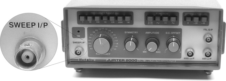
Figure 8.3 Black Star Jupiter 2000 0.2Hz–2MHz function generator. The inset illustrates the BNC connector type.
Outputs
The core purpose of a function generator is to output a test signal. In common with much audio test equipment, BNC connectors are the most commonly encountered output connectors found on function generators. The Jupiter 2000 (Figure 8.3) sports three outputs to the righthand side of the front panel. These are labelled, ‘600Ω O/P’, ‘50Ω O/P’, and ‘TTL O/P’.
As discussed in Chapter 9 – Basic Circuit Analysis, output and input impedances are important when considering the interfacing of electronic circuits. Most often low output impedance and high input impedance is to be expected in modern interfacing, and the 50 output is usually going to be the one to opt for here. The 600 output reflects the fact that historically 600 ohm to 600 ohm impedance matched interfacing was common. The TTL output is also somewhat of a historical option. TTL stands for transistor transistor logic, and refers to a particular kind of circuit architecture common in years gone by but of less importance today. As a general rule, an output like this should be avoided unless you know it is what is needed.
Controls
An analog device like the Jupiter 2000 makes for a very straightforward user interface. On the other hand, the FG085, which is a digital device, provides more functionality at the expense of higher complexity in operating it. In either case the most fundamental controls allow for the output’s shape, frequency, and amplitude to be controlled.
The commonest wave shapes provided by function generators are sine, square, and triangle. Ramp and sawtooth waves can be seen as variants of the basic triangle wave shape. Other common options include DC offset, symmetry, and duty cycle.
A typical test procedure for working with audio circuits would be as follows. Configure the function generator by selecting the sine wave shape, setting the frequency to 1kHz, and dialing the signal amplitude down to zero. Then the generator output can be connected to the input of the circuit under test, and with the input and output of the circuit displayed on an oscilloscope, the amplitude is increased on the function generator to observe the operation of the circuit.
Displays
A simple analog device such as that shown in Figure 8.3 may have no information display at all (in this case a power LED is the only indicator present). Configuration settings are read from the legends surrounding controls, and exact values may be measured externally where they are required.
On the other hand, a device such as the FG085, which incorporates a simple graphical display, can be designed to provide direct feedback on the current device configu-ration. Even a small dot matrix display can be programmed to provide a wide range of feedback and information.
Multimeters
The multimeter represents the commonest and most widely useful of all electronics test and measurement equipment. Multimeters come in a variety of types, ranging from cheap and basic to extremely expensive and highly functional. Figure 8.4 illustrates two hand-held DMMs (digital multimeters), while a benchtop unit is shown in Figure 8.5, and finally an analog multimeter (aka VOM, volt-ohm-milliammeter, and also sometimes called an Avometer ®) can be seen in Figure 8.6. No matter the shape and size, and the variety of advanced functions notwithstanding, the basic functionality provided is more or less universal – the measurement of voltage, current, and resistance.

Figure 8.4 Two examples of hand-held DMMs.
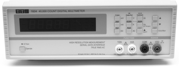
Figure 8.5 TTi 1604 benchtop DMM.
Inputs
Multimeters almost always use banana plugs for connecting test leads (see inset in Figure 8.6). There are typically either three or four banana sockets, two of which will be used for any given measurement. Usually one socket, labelled ‘COM’ – for common – is used in (almost) all measurements. Most measurements apart from current use one other, with the final one or two typically reserved for current measurements. Generally the labelling on the sockets makes clear which are to be used for any given measurement. A rare case where the common terminal is not used can be seen in the VC9805A+ unit in Figure 8.4b. In this unit temperature can be measured by attaching a special probe between the two terminals labelled ‘TEMP−’ and ‘TEMP+’.
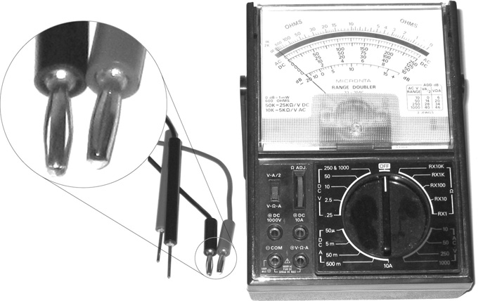
Figure 8.6 Micronta 22-204C analog multimeter (VOM), with banana plug connectors.
The VC9805A+ provides two other inputs worth mentioning. At the top right is a BJT tester (inset to the right), the three legs of a bipolar junction transistor can be inserted into the appropriate slots and a reading of the device’s gain (or hfe value) can be obtained. See Chapter 17 for more details on this important transistor parameter.
To the bottom left of the VC9805A+ front panel are two additional slots with ‘+’ and ‘−’ above them and ‘CX LX’ below them (inset to the bottom left). These inputs allow for the measurement of capacitors and inductors. By selecting the appropriate range on the dial, capacitances in farads (up to 2000µF) or inductance in henries (up to 20H) can be measured.
Outputs
Hand-held units rarely if ever have any outputs. Benchtop units may provide a serial or USB connection which can be used for data logging as well as remote control. The TTi 1604 in Figure 8.5 provides a serial interface on its rear panel and comes with a rudimentary data logging software application which allows a large number of readings to be taken over a long period of time.
Controls
On a hand-held device the main control is almost always a large rotary switch used to select between the often large number of measurement options available (the VC9805A+ features no fewer than 30 switch positions). The labelling usually makes it quite clear what can be measured in each position, although some ranges require a little more information to fully understand. As always, the user manual is a valuable resource.
The hand-held units shown both feature fully manual range selection. Many multi-meters (such as the 1604 benchtop unit from Figure 8.5) implement an auto-ranging facility where only the basic measurement type needs to be selected, and then the specific range to be used is determined by the device. This makes taking measurements an easier process but does inevitably take longer to get a result as the unit must assess the signal to be measured and determine the range to use before making and reporting the final measurement.
Whether a rotary switch or a keypad interface is being used, the selected range value (for a manual ranging device) usually indicates the maximum value which can be successfully measured in that range. What happens if that limit is exceeded can vary from range to range, and from meter to meter. Sometimes the display will flash, or display something other than a valid reading. A common out of range display for resistance measurements is a number ‘1’ displayed on the leftmost position of the display. Other meters might display ‘OFL’, meaning overflow, or some other similar indication. When measuring voltage and current in particular, it is best to avoid selecting any range lower than that required, as this can potentially overload the meter and, at best, blow a fuse. For this reason it is best to start the measurement of unknown voltages and currents at the highest range available, and work down until an optimal reading is achieved.
Generally if a range higher than the optimal is selected, a valid result will be returned; it will just not be as precise as it could be. For instance, Table 8.1 illustrates the readings obtained testing the same resistor across every resistance range available on two DMMs. The results make it clear that the resistor in question is a nominal 1k component. It is in fact a 1k carbon film device with a tolerance of 5%, and as such appears to be within spec. See Chapter 12 – Resistors, to expand on tolerances and resistor specifications.
Table 8.1 Resistance measurement results for two hand-held DMMs. The component under test is a 1kΩ, 5% carbon film resistor
| 2.0 | 2000/2ka | 20k | 200k | 2M | 20M | 200M | |
| Tenma 72-7770 | 1 . | 976 | 0.98 | 01.0 | – | 0.00 | 01.0b |
| Vichy VC9805A+ | 1 . | .980 | 0.98 | 00.9 | .001 | 0.00 | – |
Displays
A multimeter will either have a large moving needle display (for a VOM) or a numerical readout (for a DMM). These digital displays can incorporate all sorts of useful icons and glyphs in addition to the primary numerical readout. They also usually incorporate a minus sign. Most DMMs are designed to handle DC voltage and current measurements in either polarity. Analog meters on the other hand (where the needle’s resting position is almost always at one extreme of the meters movement) should only be connected in their correct polarity, to avoid damage to the meter.
Analog meters are widely considered obsolete, as digital devices have taken over. Digital meters offer many advantages over their analog forebears, in terms of resolution, accuracy, repeatability, ease of use, flexibility, and robustness. There are still a couple of places where an analog movement may still have the edge over a digital readout. While single readings favour the digital format, slow moving signals and trends may be easier to detect and follow using a moving needle – a kind of halfway house on the road to oscilloscope functionality. A needle movement can also make it easier to spot and assess small glitches – for example in determining the polarity of an electric guitar pickup by observing the direction of needle movement when the pickup is touched with a metal rod (e.g. a screwdriver).
Common Measurement Tasks
Most measurements are performed by selecting the appropriate range on the multi-meter, connecting the two test leads to the appropriate points, and reading the result off the multimeter display.
Resistance
Resistance measurements must not be performed with power applied to the device or component being tested. Most commonly a single resistor in isolation is the target of such a measurement, although it can also be useful to measure the resistance between two points in a circuit. When making in-circuit measurements it is important to assess the entire circuit region surrounding the test points. While the test probes may be connected on either side of a single resistor in a circuit, it should not be assumed that such a measurement will automatically return the value of this resistor. The circuit should be examined to see if other parallel resistance paths might exist, which will potentially affect the result. As indicated in Figure 8.7a, the best way to measure a resistor is to do so with it removed from any circuit it may be a part of. This is not always possible, but is the ideal.
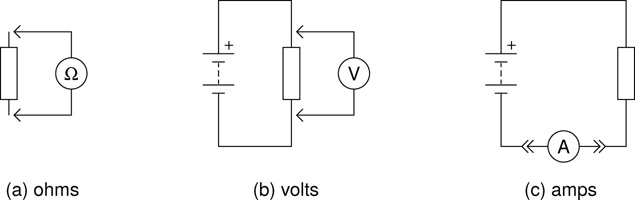
Figure 8.7 Connecting a multimeter to measure resistance, voltage, and current.
When using an auto-ranging multimeter it is sufficient to simply select the ohms range and let the meter do the rest. For a manual meter it will usually be necessary to switch through several range settings in order to get the best possible reading, as illustrated by the results presented in Table 8.1 above. Clearly in this case the 2k range gives the best result, maximising resolution and hence precision. Switching down a range takes the meters beyond their maximum readings, while going up a range, while producing a valid result, does loose a decimal point of precision.
Voltage
Voltage measurement, Figure 8.7b, involves selecting the appropriate range, and bridging across two points in a circuit with the probes of the multimeter. With voltage and current measurements it is very important to know whether it is a DC or an AC signal which is to be measured, and to set the meter correspondingly. While most meters provide for both AC and DC voltage measurements, AC current measurement is less commonly available (the Vichy in Figure 8.4 provides it but the Tenma does not).
Current
Current measurement is the most involved of the three primary measurement types. It is necessary to make a break in the circuit path to be analysed, and to insert the meter into the circuit, as shown in Figure 8.7c. The most common place to do this is in either of the two connections between circuit and power supply. This test can be used to determine the overall current draw of a circuit, which can be useful information, both in checking that there are no faults or errors in the circuit causing an unexpected current drain, and in assessing the powering requirements for a circuit – is it, for instance, suitable for battery powering or would it drain batteries too quickly?
Continuity
While volts, ohms, and amps measurements are the core functionality of any multimeter, one of the most useful functions provided by most meters is the continuity or buzz tester (Figure 8.8). In electrical terms, continuity means a low resistance electrical connection. The action of a buzz tester is very straightforward; if a sufficiently low resistance is detected between the measurement probes then a buzzer within the meter sounds. Typically the threshold for a continuity tester is somewhere in or around the 10 to 30 region. At resistances below this limit the buzzer activates; thus a buzz should always be heard when the test probes are touched together while the multimeter is in this mode.

Figure 8.8 Multimeter continuity test mode. The meter beeps if a sufficiently low resistance is connected.
Continuity testers are particularly useful for testing cables and circuit boards. Any time solder has been applied, it can be a worthwhile exercise to ‘buzz out’ the work before deeming it complete. It is important to check both that all the required connections are present and solid, and that there are no unwanted connections due to solder going somewhere that it shouldn’t have. The latter is particularly common when soldering tightly laid out stripboard circuits, as is discussed in Chapter 10.
Diode
The diode test range on many hand-held multimeters shares a switch position with the buzz tester, and is typically indicated by a combined symbol as in the upper left inset in Figure 8.4. Diodes are one of those components where the orientation of the device is significant, so it is important to observe the connection order when interpreting the results of a diode test, see Figure 8.9. For a diode in good working order, the reading indicates the forward voltage required to get a small amount of current (typically about 1mA) to flow through the device. This voltage varies for different types of diodes. See Chapter 16 – Diodes, for more details on diode behaviour and typical characteristics.
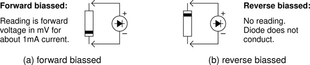
Figure 8.9 Multimeter diode test mode. In forward bias, the meter reports the voltage required to get a small current to flow.
Oscilloscopes
Oscilloscopes are one of the most variable pieces of standard lab equipment, both in terms of the functionality they provide, and in terms of the interface used to access and control that functionality. In this section, all the bells and whistles which any given device may provide are ignored. The fundamental functionality and how it is controlled stays fairly consistent across the gamut of oscilloscopes likely to be encountered. This involves displaying a steady picture with the optimum horizontal and vertical on screen sizing. While the multimeter presents a single reading, the oscilloscope allows a changing signal to be displayed graphically over a period of time.
Oscilloscopes come in a variety of form factors. Old analog scopes are large and heavy, with a very deep body in order to accommodate the long cathode ray tube used for the display screen. An analog scope is often referred to as a CRO or cathode ray oscilloscope. More modern digital scopes are usually called DSOs or digital storage oscilloscopes, because they can store and redisplay a signal plot after the signal is gone. USB scopes provide signal capture and A-to-D conversion hardware, but no screen. They rely on an attached computer for control and display purposes. Soft scopes on the other hand are software applications without any dedicated hardware. They take their input signals from standard audio interface hardware, and so are only usually of any use up to audio frequencies (below about 20kHz or so). Even a basic hardware scope will usually extend up to at least a couple of hundred kilohertz, and more likely to a couple of megahertz or more. Even when working exclusively with audio circuits this extended oscilloscope bandwidth can be useful. High frequency noise can be a problem which needs to be visualised in order to be addressed effectively.
Figure 8.10 illustrates the major controls found on most analog oscilloscopes. Most of this functionality is shared across digital scopes too, with just one or two exceptions. Both analog and digital types can exhibit a wide array of additional functionality, but the basic controls covered here allow the user to make all of the basic measurements typically required. There are five groups of controls shown in the figure: sweep, mode, trigger, channel 1, and channel 2. Most oscilloscopes have two channels, allowing two signals to be viewed simultaneously. This common configuration is assumed in the example provided here.
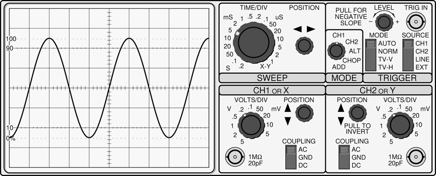
Figure 8.10 Typical oscilloscope front panel controls. Oscilloscope interfaces and functionality vary greatly, but most of these controls are always present in some form.
Mode
The Mode section just has a single five-way rotary switch, used to set the device’s operating mode, selecting which channels to display and how to display them.
CH1: display channel one only
CH2: display channel two only
ALT: display both channels (default, best at higher frequencies)
CHOP: display both channels (prevents flicker at lower frequencies)
ADD: display the sum of the signals on the two channels
Trigger
The trigger section controls how and when a trace starts drawing on the screen. Getting the trigger setup wrong results in the trace continually running across or jumping around the screen (see Figure 8.11d). A well configured trigger gives a good solid trace without any movement. The trigger settings generally apply to both channels. Some more advanced oscilloscopes allow for offset or independent triggering of channels.
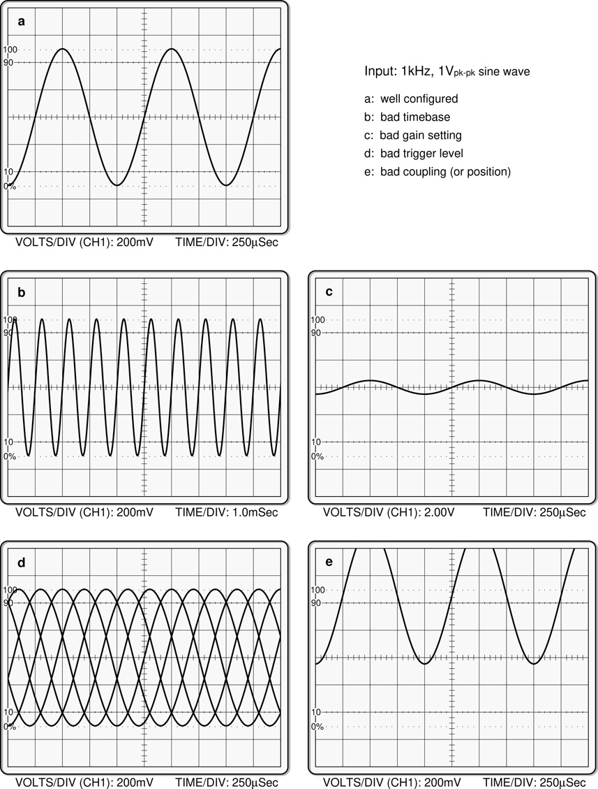
Figure 8.11 Effects of some important oscilloscope settings.
SOURCE: selects what signal is used in order to generate the trigger which initiates the trace. CH1 is the right choice in most situations.
MODE: controls the rule used to initiate triggering. AUTO is usually the right choice.
LEVEL: chooses the vertical position on the screen at which triggering will happen. The middle of the pot rotation is the best place to start. Adjust up and down if needed, until a steady trace is obtained.
SLOPE: can be negative or positive, controlled here by pulling out or pushing in the level knob. Usually best left positive (rising) unless it is specifically necessary to zoom in on the negative slope (falling edge) of the signal.
Channels 1 and 2
Each set of channel controls is usually more or less identical. In this case only a channel two invert option differentiates the pair. The channel controls are primarily about adjusting the vertical aspects of the display (Figure 8.11c). Three controls are shown here (plus the channel two invert option), as well as the BNC connectors where the probe is attached for each oscilloscope channel.
VOLTS/DIV: (volts per division) sets the vertical scaling of a channel. There are eight divisions marked out on the screen from bottom to top. To find a signal’s peak to peak amplitude, count the number of divisions it covers, and multiply by the volts per division setting. If a times ten probe is used (see below), multiply the answer by ten. Digital scopes can usually be told to make this correction automatically.
POSITION: allows the whole trace to be moved up and down on the screen. Good for spacing the two channels to make the most of the available screen space. Channel two here can also be inverted by pulling out the position knob.
COUPLING: GND disconnects the signal, and connects the channel to ground, producing a flat line trace (used with the position control to zero a channel). AC coupling allows only the AC portion of a signal through. Any DC bias is removed. DC coupling allows both AC and DC components through. Assuming the channel is properly zeroed to start with, then a display like Figure 8.11e using the DC setting, will change to Figure 8.11a when coupling is switched to AC.
Sweep
Just as the ‘channel’ controls are about adjusting the vertical display, so the sweep controls are about adjusting the horizontal display. Figure 8.11b illustrates a trace with poor sweep settings. The sweep controls are shared by both channels.
TIME/DIV: (time per division) sets the horizontal scaling of the channel. There are ten divisions across the screen. The period of a signal is determined by counting the number of divisions covered by one cycle and multiplying by the TIME/DIV setting. Frequency is then easily determined as one over period (Eq. 5.2). In the example illustrated in Figure 8.10, the final position sets the scope into X-Y mode (see below).
POSITION: allows the traces to be moved left and right on the screen. Good for aligning a plot’s crossing point or scanning to out of view data. Digital scopes in particular often capture more data than is plotted across the width of the display area.
X-Y Mode
Most two channel scopes can be placed into a special mode where, instead of displaying signals plotted against time, the display shows channel one plotted against channel two. This mode can be useful in a number of applications including examining the phase relationship between two signals. It can also be used to display a diode’s i-v curve, as described in Learning by Doing 16.2 (p. 281).
Oscilloscope Probes
The standard oscilloscope probe consists of a spring loaded hook terminal, which can often be removed to reveal a pointed contact pin beneath (Figure 8.12). Coming off to the side is a clip lead. The main contact is connected to the point in a circuit which is to be examined while the clip lead must be connected to a voltage reference point, usually the circuit’s signal ground.
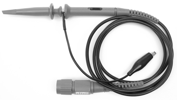
Figure 8.12 A standard ×10 oscilloscope probe. The black switch on the handle is the times one/times ten selector.
It is important to note that in a standard mains powered oscilloscope the ground clip lead is connected directly to earth ground through the mains power cord ground wire. This means that if a circuit also connected to earth ground is being examined the ground clip lead must only be connected through to this earth ground point in the circuit under test. There are various ways of overcoming this limitation (see Tektronix, 2011), the simplest of which is to use a battery powered oscilloscope. These issues are particularly mentioned in the same Learning by Doing 16.2 exercise mentioned above, which describes how to use an oscilloscope to visualise a diode i-v curve.
The ×10 probe (times ten probe) is the most common type of probe encountered in conjunction with a standard oscilloscope. A switch on the handle labelled ‘×1 ×10’ switches in and out an attenuation network which in the ×10 position reduces the input signal by a factor of ten. The ×10 position also enables an adjustable compensation circuit which allows for the best possible accuracy of signal reproduction. Generally it is best to use this mode where possible, but it is important to remember that the signal amplitude readings taken must be re-scaled times ten (hence the name) to arrive at the true reading. In other words, a reading of 0.5V is actually 5.0V. As mentioned above, while this must be done manually when using an analog scope, a digital scope can usually be set up to perform the calculation automatically.
Audio Analysers and Advanced Test Gear
The systems from Audio Precision probably represent the de facto standard for audio test and measurement equipment. Prices for even the most basic systems start at several thousand euros. Many other manufacturers also offer audio analysers of various descriptions. The Keithley 2015-P Audio Analysing DMM shown in Figure 8.13 is one such device, providing measurement functions including harmonic distortion and spectrum analysis. Equipment such as this generally lies beyond the grasp of all but the specialist audio electronics practitioner, and details of its uses and utilisation fall well outside the scope of this book.
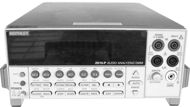
Figure 8.13 Keithley 2015-P Audio Analysing DMM.
References
G. Ballou, editor. A Sound Engineers Guide to Audio Test and Measurement. Focal Press, 2009.
E. Brixen. Audio Metering: Measurements, Standards and Practice. Focal Press, 2nd edition, 2011.
N. Crowhurst. Audio Measurements. Gernsback Library Inc., 1958.
J. Dunn. Measurement Techniques for Digital Audio. Audio Precision, 2004.
B. Metzler. Audio Measurement Handbook. Audio Precision, 2nd edition, 2005.
Tektronix. Fundamentals of Floating Measurements and Isolated Input Oscilloscopes. Tektronix, 2011.