12 | Resistors
The resistor is the simplest and also the most fundamental of all electronic components. It is designed to have a constant resistance across all frequencies and under all normal circuit conditions (within reason). Resistors limit the amount of current flowing through them and they drop voltage across their terminals. Voltage drop is the term used to talk about the difference in voltage between two points in a circuit, also commonly referred to as the potential difference between the two points.
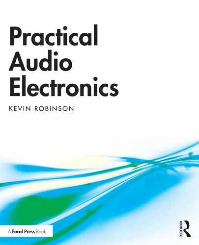
Resistors come in many shapes and sizes, but the most common format used for handmade electronics is the little dumbbell with coloured stripes on its body and leads sticking out from either end as in the image in Figure 12.1a. These are called through hole resistors and they are designed to be used by bending the legs, inserting them through holes in a circuit board, and then soldering them in place on the boards reverse side.
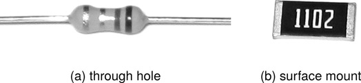
Figure 12.1 A through hole resistor and a surface mount (SMD) resistor.
For comparison, Figure 12.1b shows the kind of resistor typically used in modern machine assembled circuits. These resistors look like small chips of black plastic, and are called surface mount devices or SMDs. They come in different sizes but tend to be very much smaller than typical through hole resistors. Some people do hand solder the larger of these surface mount devices but it is a tricky skill to master and is not addressed in this book. The shiny regions at either end of the device are the solder pads where it is soldered into the circuit, and the number indicates the value of the resistor in ohms. The first two digits are the start of the number and the third digit tells how many zeros to add. So in the case of Figure 12.1b the value is thirty followed by three zeros, i.e. thirty thousand ohms or 30kΩ. By contrast the resistance of a through hole device is determined by decoding the coloured stripes on its body. The interpretation of resistor colour codes is examined shortly.
Two different symbols are commonly used to represent resistors when drawing circuit diagrams. In this book the convention of a rectangle is used exclusively as in Figure 12.2a. The zigzag symbol in Figure 12.2b is used widely elsewhere and indeed both are encountered regularly. There is no difference between the meanings of these two alternate forms of the resistor circuit symbol.
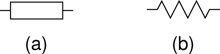
Figure 12.2 Circuit diagram symbols for a resistor.
The resistance value measured in ohms is the most important quantity describing any given resistor. There are however quite a number of characteristics which together define the precise nature and performance of any resistor. In addition to the resistance value, these include such things as its manufacturing tolerance, power handling capability, composition, and temperature coefficient. Self (2015, pp. 44–63) provides an examination of the effects of tolerance, along with consideration of the noise and distortion contributions of resistors in audio circuits. The following sections examine the most important facets of each of the above characteristics in turn.
E-Series Preferred Values
Certain particular resistance values turn up again and again, such as 47 and 82. There is good logic behind the use of such commonly encountered and yet strangely irregular numbers. Resistors come in values from a fraction of an ohm up to several million ohms (the most commonly used values are generally in the range 100Ω to 1MΩ). It would be impractical for manufacturers to offer every conceivable resistor value in these ranges, and so this has led to the use of the E-series preferred values. These series specify sets of standard values. Each series uses a different number of values to cover a decade (a multiple of 10). So for instance the E3 series includes three values while E12 consists of twelve. The standard series extend up to E192 for very precise resistance values, but E12 and E24 are probably the two most commonly used sets of values.
Table 12.1 shows the values in the first three series: E3, E6, and E12. There is certainly no need to remember these values but the commonest, like 10, 22, 33, and 47 will quickly become familiar to anyone regularly working with electronic components. Clearly it makes sense for smaller values to be spaced more closely and larger values to be more spread out. While a gap of twenty ohms might be reasonable when for instance going from 100Ω to 120Ω, providing the option of say both one million ohms and one million and twenty ohms makes less sense. The most logical way to choose what values to make readily available is to use a multiplication factor to go from one value to the next. In this way the step size slowly and steadily increases as the resistor values increase.
Table 12.1 The first three resistor E-series preferred value series
E-series |
Preferred values |
|||||||||||
E3 |
10 |
22 |
47 |
|||||||||
E6 |
10 |
15 |
22 |
33 |
47 |
68 |
||||||
E12 |
10 |
12 |
15 |
18 |
22 |
27 |
33 |
39 |
47 |
56 |
68 |
82 |
So in order to work out what values should be included in a given series the first thing to do is to decide on the number of values to be available in each decade (i.e. the E3, E6, E12, E24 thing). Next a bit of maths gives the necessary factor, and then any value can be multiplied by this factor and the answer rounded to the nearest sensible number to give the next value in the series (the maths will give answers like 14.677992... – that one is the third in the E12 series, so let’s just call it 15). Notice how the gaps between values increase going up through the E12 series shown in Table 12.1, and remember of course that the next step up will be from 82 to 100, a step size of eighteen, the biggest yet. Similarly, the next values heading down from 10 will be 8.2, 6.8, and so on. Thus standard values in any range can be specified, going up as high or down as low as is needed.
Tolerance
Every resistor will have an actual value which is slightly different from its specified value due to the limitations of the manufacturing process. Resistors are manufactured to a certain tolerance, the commonest being ±5% and ±1%. The tolerance indicates the guaranteed maximum deviation from the labelled value. Five percent of two hundred and twenty is eleven, so a 220Ω resistor with a ±5% tolerance might actually have a value anywhere in the range 220 ± 11 (i.e. 209Ω on up to 231Ω). Resistors with tight tolerances will generally cost more. In most of the circuits considered in this book (and in many circuits in general) precise values are not crucial to the operation of the circuits, so tolerances are not usually of any great concern, and ±1% or even ±5% will usually be quite sufficient. It is still worth being aware of their existence and their values for the components used.
There is a logical relationship between the tolerance and the E-series. Consider two resistors, one 220Ω and the other 230Ω, both with ±10% tolerance. Ten percent of 220 is 22 so the 220Ω resistor might actually have a value anywhere between 198 and 242. Similarly with ten percent of 230 being 23, the 230Ω resistor can fall anywhere in the range 207 to 253. Now clearly the 220Ω resistor is supposed to be the smaller of the two but its largest allowed value (242Ω) is significantly bigger than the smallest allowed value of the nominally larger resistor (207Ω). It would make little sense to have these two resistors in the same set, so maximum sensible tolerances for each E-series can be defined which avoid large overlaps in the possible values of adjacent nominal values. These maximum tolerances are shown in Table 12.2.
E-series |
Maximum typical tolerance |
E3 |
±50% tolerance (no longer used) |
E6 |
±20% tolerance (seldom used) |
E12 |
±10% tolerance |
E24 |
±5% tolerance |
E48 |
±2% tolerance |
E96 |
±1% tolerance |
E192 |
±0.5% and tighter tolerances |
Notice that Table 12.2 indicates a maximum standard tolerance of ±10% for the E12 series. From Table 12.1 the next value up from 22 in the E12 series is seen to be 27. Applying the ±10% bands to these two standard values gives allowed ranges of 19.8– 24.2, and 24.3–29.7 respectively. So even in the very worst case scenario (which is itself extremely unlikely) a nominal 22Ω resistor with a ±10% tolerance will at least remain slightly smaller than a nominal 27Ω resistor with a ±10% tolerance. Most resistors these days are actually ±5% or ±1%, even when sold as E12 series components, so generally the actual values of resistors match their nominal values quite closely.
Resistor Colour Codes
The coloured stripes on a standard through hole resistor tell two things: the resistance value and the manufacturing tolerance. It is not necessary to remember the colour codes, they can always be looked up as and when they are needed. It is however useful to know how to interpret them. The code on a standard resistor will consist of either four or five coloured stripes. The colours can be interpreted using Table 12.3.
Colour |
Digit |
Multiplier |
Tolerance |
Black |
0 |
×1 |
– |
Brown |
1 |
×10 |
±1% |
Red |
2 |
×100 |
±2% |
Orange |
3 |
×1k |
±3% |
Yellow |
4 |
×10k |
±4% |
Green |
5 |
×100k |
±0.50% |
Blue |
6 |
×1M |
±0.25% |
Violet |
7 |
×10M |
±0.10% |
Grey |
8 |
×100M |
±0.05% |
White |
9 |
×1G |
– |
Gold |
– |
×0.1 |
±5% |
Silver |
– |
×0.01 |
±10% |
None |
– |
– |
±20% |
The last two stripes always have the same meaning – the second last stripe is the multiplier and the last stripe is the tolerance. This leaves either two or three colours which get turned into the first two or three digits of the value. So a five stripe code allows for the greater precision needed in E48 series and above, where numbers like 105 and 226 are encountered.
So for instance the 220Ω ± 5% resistor mentioned above might have either a four or five colour code depending on the E-series it has been manufactured as a part of. The four colour code would be: Red, Red, Brown, Gold, while the five band code would be: Red, Red, Black, Black, Gold. However it is worth noting that a five band code is more likely to be found on a ±1% tolerance resistor, so the last stripe would be brown instead of gold.
In theory there should be a slightly wider gap between the last two stripes so that it is possible to tell which way round to read the code but in practice it is often difficult to differentiate this larger space. On ±5% resistors this isn’t a problem because Gold does not represent a digit and so can not appear as the first stripe. With ±1% resistors it is more problematic as Brown is also a valid digit.
It is worth saying however that the sometimes tricky task of deciphering colour codes is often unnecessary. With loose resistors it will usually be easier to use an ohm meter to measure the value. However with resistors which are soldered into a circuit, using a meter is not a reliable guide, as other components in the circuit may contribute to the answer which the meter provides. Sometimes a little bit of investigative work is needed to confirm the actual value.
Power Rating
As with all components, when current flows through a resistor it heats up. The power rating indicates how much heat it can dissipate before it runs the risk of being damaged. Standard resistors can usually handle between about 125mW and 0.6W of power safely. The power ratings of standard through hole resistors are relatively modest. The three components shown in Figure 12.3 have, going from top to bottom, power ratings of 600mW, 250mW, and 125mW. The smallest of the three, at barely 3.5mm long, is a slightly less common format, and the upper two exemplify by far the most usual range of through hole resistors encountered.
Figure 12.3 Standard through hole resistor power ratings correlate closely with the size of the components. The three resistors shown are rated at, from top to bottom: 600mW, 250mW, and 125mW.
For higher dissipations physically bigger components are needed, possibly with integrated heat sinks to help get rid of excess heat. Figure 12.4 shows examples of three types of power resistor with different power ratings.

Figure 12.4 Power resistors.
Power resistors are usually of wire wound construction (see the next section), often encased in a ceramic material which can handle high temperatures. For the highest power handling capabilities they can also be encased in an aluminium housing and, like the 25W component shown in Figure 12.4c, mounting holes may be provided to allow the component to be bolted onto an additional external heat sink. This provides extra heat conduction away from the resistor keeping it cooler and avoiding failure. High power components such as these can get very hot indeed when working hard and extra care must be taken when investigating such a circuit. The three high power components shown in Figure 12.4 are capable of dissipating five, eight, and twenty five watts respectively.
Material and Temperature Coefficient
The commonest constructions for standard resistors are carbon film and metal film but there are others. High power resistors will often be of wire wound construction for instance. Other makeups have also been employed. Carbon composition used to be common but has poor characteristics in many respects and is rare these days. More exotic materials are also used to provide better performance in various characteristics but these types tend to be very much more expensive and are only really of interest to manufacturers of high end gear and precision measurement equipment.
While an understanding of what these various materials and methods of construction entail is by and large unimportant, it can be useful to recognise the terms and have an appreciation of some of the more important implications of the particular types of resistors used in a project. Of the two most commonly used materials carbon film tend to be cheaper than metal film, but also poorer on most counts, with looser tolerances (typically ±5% vs. ±1% for metal film) etc. Thick film and thin film variants also exist. As a general guide, avoid carbon composition and thick film components, and choose metal film over carbon film unless the small cost savings of using carbon film are important.
One last component characteristic worth mentioning briefly is the temperature coefficient. A resistor’s temperature coefficient indicates how its value changes as its temperature changes. A typical temperature coefficient may be quoted as ±50ppm/°C, where ppm stands for ‘parts per million’. This value thus indicates that for every °C change in temperature, the resistance may change by up to 50 millionths of the total value, e.g. a nominally 1MΩ resistor might change in value by up to ±50Ω for each °C change in its temperature. Typically with resistors as the temperature goes up the resistance goes up, and as the temperature goes down the resistance goes down. This is called a positive temperature coefficient. There are also components which exhibit a negative temperature coefficient (as temperature goes up, resistance goes down, and vice versa). Both these property are sometimes used to good effect in specialised components, but on the whole, for standard resistors, the smaller the temperature coefficient the better. Ideally the resistance should not change at all as the temperature changes, but in reality it will always vary to some extent.
Electrical Behaviour
The details of how resistors behave and how they are analysed in particular circuits are addressed in more detail in Part II. Here just a brief examination of their electrical characteristics is presented. In particular, two important aspects of a resistors behaviour are touched upon, described here under the headings ‘Transfer Function’ and ‘Frequency Response’.
Transfer Function
A transfer function is a general description of the behaviour of a device or system, presented in terms of how the output of the system changes as the input to the system is altered. This kind of analysis can take on many specific forms depending on the nature of the system under consideration. In addressing the electrical behaviour of a simple resistor, the input is considered as a voltage applied across the ends of the resistor, and the resulting output is quantified in terms of the current which flows through the resistor as a result of the applied voltage. (This particular relationship, plotting current against voltage is often also referred to as an i-v characteristic.) As discussed in Chapter 2, voltage can be thought of as the electrical push or pressure, and current is the flow of electricity which comes about as a result of that push.
So the transfer function of a resistor can be presented in terms of current against voltage. This relationship is illustrated by the graph in Figure 12.5 which shows that the current (measured in amps) rises as the voltage (measured in volts) rises, and falls as the voltage falls. The graph is a straight line, which represents a linear relationship between the current flowing through the resistor and the voltage which is causing it to flow. The line passes through the origin; when the voltage is zero, zero current flows. The slope of the line represents the size of the resistor (measured in Ohms). A bigger resistor is represented by a shallower slope, and a smaller resistor is represented by a steeper slope. Later on, in Chapter 9, this relationship is formalised with Ohm’s Law, one of the most important and useful rules for analysing circuits. For now it is more important to develop a general understanding of the behaviour, and to be able to visualise in general terms how a changing voltage across a resistor will alter the amount of current flowing through it. While this is a general rule in electronics, more voltage equals more current, more electrical components do not exhibit the linear relationship which is illustrated here. Generally more complex behaviour is to be expected.
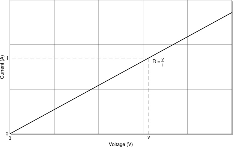
Figure 12.5 Resistor transfer function.
Frequency Response
As the focus of this book is audio electronics, frequency response is an aspect of the behaviour of any circuit or component which is of great interest. Music, and audio in general is all about the frequency content of the signals being encountered. An amplifier wants to preserve the frequency content of a signal, an EQ aims to alter the frequency balance in a controlled way, and a distortion effect looks to introduce new frequencies related to those already present.
As such it is clear that an understanding of how various components affect the frequency content of a signal is of great import. It should be of little surprise that the resistor, being the simplest of all components, presents very straightforward frequency behaviour, as shown in the frequency response graph presented in Figure 12.6.
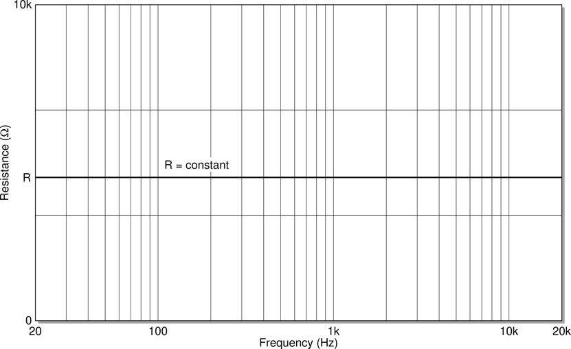
Figure 12.6 Resistor impedance vs. frequency. In isolation this is an uninteresting graph. The impedance-frequency relationship becomes very important once capacitors and inductors are added to the mix as shall be seen in the next chapter. An appreciation of the differences in behaviour between these three components is vital to understanding the operation of many key audio circuits.
The frequency response of a device or system represents how that system behaves when presented with signals of different frequencies. It can be thought of as a particular kind of transfer function where the question is how the level of the output changes as the frequency of the input signal is changed. As can be seen from the graph, the answer in this instance is that the output level remains constant regardless of the frequency of the input. This is in contrast to the behaviour of the next two components which are examined: capacitors and inductors. In that case very clear and predictable variations are observed, which lead to the conclusion that capacitors and inductors are ideal components for building filters – circuits which modify the frequency balance of a signal.
The frequency response in Figure 12.6 is shown in terms of how the resistance (here called impedance, don’t worry about the difference for now) measured in Ohms changes as the frequency of the input signal changes. As has already been stated, in this case there is no change. In Chapter 13 on capacitors and inductors the same frequency response graph reappears with two new plots added, in order to compare the behaviours of these three important components. This leads naturally to an understanding of how some very simple filter circuits can be designed.
Series Rule and Parallel Rule
When analysing circuits it is often necessary to work out the total resistance of a number of resistors wired in various configurations. Even the most complex resistor network can be reduced to a single resistance value through the successive combination of pairs of resistors wired either in series or in parallel.
Two simple rules are used to achieve this, usually referred to as the resistor series and parallel rules. What these two rules are saying is that the two resistors in series or parallel could be replaced by a single resistor whose value is given by the appropriate rule without changing the operation of the circuit.
Series Rule
The series rule for resistors just says that the combined resistance of two resistors wired one after the other (see Figure 12.7) is the sum of the two individual resistor values.
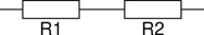
Figure 12.7 Resistors in series.
For two resistors in a circuit to be candidates for an application of the resistor series rule a number of conditions must hold. The two resistors must be directly connected at one end and must not be directly connected at their other ends (or they would be in parallel). It also must be the case that there are no other connections into the point where the two resistors join. If these conditions hold then the two resistors may be replaced by a single resistor without altering the operation of the circuit.
Parallel Rule
The parallel rule allows a combined value to be calculated for two resistors wired up side by side as in Figure 12.8. Here the calculation is a little more involved though still not what might be call complex.

Figure 12.8 Resistors in parallel.
There is another formulation of the parallel rule which allows for the combination of more than two resistors in parallel simultaneously but there is no need to confuse the issue by introducing that equation here. On the rare occasions when three or more parallel resistors require summing, multiple applications of Eq. 12.2 yields the correct result. The form of this alternative version, along with a proof of its equivalence, is examined in the highlighted Box 12.1 (p. 212).
Example
As a simple example of the application of these rules consider the circuit shown in Figure 12.9. Equipment A is to be connected via a cable to equipment B. However the output and input impedances do not match and so resistors R1 and R2 are inserted at the output of equipment A as shown. The task is to ensure that the modified output impedance seen by equipment B has the correct value.
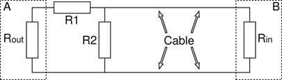
Figure 12.9 Series and parallel law example.
Equipment B looking back down the cable sees the combined impedance of R1, R2, and Rout the output impedance of equipment A, but how do these three impedances combine? First it is necessary to add R1 and Rout in series.
The resulting resistance is in parallel with R2, and so they need then to be added using the parallel rule to give the final answer.
Combining these two equations into a single calculation gives
This particular example describes a simple circuit used to connect two pieces of equipment with different digital interfaces, as described in Bohn (2009). Equipment A has an AES digital output and equipment B has an S/PDIF digital input. The former has an output impedance of 110Ω while the latter has an input impedance of 75Ω. Digital connections like this prefer to have matched impedances (i.e. the same output impedance at one end as the input impedance at the other).
If R1 is set to 330Ω and R2 is set to 91Ω a suitable match is achieved,
and so it is clear that the series and parallel rules have here been successfully applied to confirm that the suggested values for R1 and R2 will indeed result in a suitable resistance at the AES digital output of equipment A, as seen from the other end of the cable at the S/PDIF input of equipment B.
Voltage Divider Rule (VDR)
The next step in the simple analysis of resistor circuits involves calculating the voltage which will appear at the midpoint of two resistors in series given the voltages at either end. This question can be considered in two parts. First the more straightforward case is examined where the voltage at one end equals zero volts, with an arbitrary voltage applied to the other end. This is then generalised to the case where arbitrary voltages may appear at both ends.
The circuit for the first case is illustrated in Figure 12.10. With the voltage Vin applied at the top of R1, and the bottom of R2 connected to ground (zero volts), the question which is to be answered is what is the voltage Vout which will appear at the junction of R1 and R2? There is a simple calculation needed to find the answer, and the equation is given in Eq. 12.3.

Figure 12.10 Simple voltage divider where the voltage at one end equals zero volts.
This basic configuration appears very often is real circuits. An attenuator or ‘pad’ circuit used to reduce the level of a signal by a given amount as it passes from one device to another might be no more than the simple voltage divider circuit shown here.
An obvious generalisation of this arrangement is when the voltage at the bottom of R2 is not zero, in which case the calculation becomes just slightly more complicated. This variation is shown in Figure 12.11, and the modified calculation is given in Eq. 12.4.
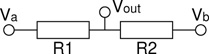
Figure 12.11 Generalised voltage divider configuration, where Vb 6= 0.
It is always worth developing a sense for roughly what the answer should be. This helps greatly in gaining a deepened understanding for the behaviour of ever more complex circuits as they are encountered. The basic rules remain unchanged no matter how elaborate the circuit. It is also well worthwhile getting into the habit of performing what is sometimes referred to as an ‘idiot check’ whenever a calculation is performed in order to confirm the answer arrived at is at least in the right ballpark. Familiarity with expected behaviour helps greatly in this regard.
In order to utilise an idiot check it is necessary to be able to apply some general rules. The first thing to remember is that the voltage at the mid point will always lie somewhere between the voltages at either end, and the second useful rule is that bigger resistors have larger voltages across them and smaller resistors have smaller voltages across them. If the two resistors are equal then the voltage at the middle is halfway between the voltages at either end. Likewise if R1 is twice the size of R2 then it has twice the voltage across it, and so Vout will be two thirds of the way from Va to Vb.
Variable Resistors
Variable resistors are extremely useful. They consist of a strip of resistive material with a terminal attached at each end of the strip, and a third terminal attached to a moving contact which connects to the strip. This contact can be positioned and repositioned at different locations along the strip to provide a continuously variable resistance between the third terminal and each of the two end terminals.
Variable resistors come in many shapes and sizes. Figure 12.12 shows some examples: a) is what is called a potentiometer or pot, and is the kind of device which might be found under a volume control for instance, b) is called a fader or linear fader, because it is moved in a straight line instead of rotating as in a pot, c) is variously referred to as a preset, trimmer, or trim pot, and while a) and b) usually provide user controls, presets are used for calibration of a circuit. They are usually intended to be adjusted when the circuit is first built and then left alone unless a recalibration of the circuit is ever required.
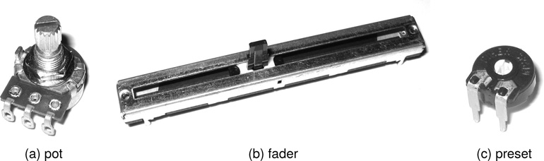
Figure 12.12 Examples of three types of variable resistor.
There are a number of variations on the circuit symbols which may be used in drawing variable resistors in circuit diagrams. Figure 12.13 shows four possibilities, two for pots and faders, and two for trimmers, although the first pair will quite often be used when a trimmer is intended in a circuit. Sometimes it is necessary to assess the context and the function being performed by the variable resistor in order to decide what style to use.
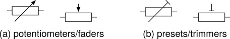
Figure 12.13 Variable resistor symbols.
The reason there are two symbols for each type is that sometimes a variable resistor is connected into a circuit using only two of its terminals, and sometimes all three are used. The symbols may be a little confusing at first since when only two terminals are used it will always be the variable one plus one of the two others, but in the symbol it looks like the two end terminals are used and the variable one is left open. This would of course make no sense as the device would then be acting as a fixed value resistor and not utilising its variable function at all.
A common practice when only two terminals are needed is to attach the unused terminal directly to the variable terminal. This makes no functional difference to the circuit but can be beneficial in reducing the noise sometimes generated when adjusting a pot (especially older pots with accumulated dirt). It can also be beneficial in the event that the moving contact in the pot breaks. The circuit will then still operate, it will just behave as if the pot has been rotated all the way to the end and left there permanently – not great but better than the alternative of an open connection.
Generally a pot can be thought of as being used to perform one of two different functions based on the way it is wired, either a potential divider or a variable resistance. In the case of a potential divider (or voltage divider) the three terminals are wired into three different points in the circuit in which case the middle (variable) contact acts as a voltage tap point providing a voltage somewhere between the voltages found at the two outer terminals. When used as a variable resistance only two terminals are actually needed, the variable one and one of the outer ones. The second outer terminal is often wired together with the variable terminal for the reasons explained above but this connection plays no role in the actual functioning of the circuit.
Pot Tapers
The final question which needs to be addressed is that of how the resistance changes as the variable resistor is adjusted. This characteristic is called the device’s taper. The logical and most common behaviour is that the amount of movement and the amount of change in resistance are directly proportional. This is called a linear taper but it is not the only possibility, as illustrated in Figure 12.14.
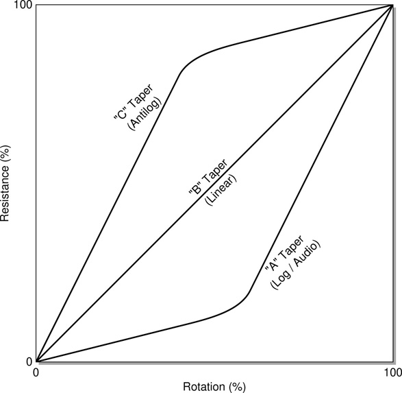
Figure 12.14 Graph showing three different potentiometer tapers.
The linear taper or ‘B’ taper says that the percentage rotation and the percentage variation in resistance between the terminals track in a linear fashion. However sometimes this behaviour does not provide satisfactory results. A common situation encountered especially in less expensive equipment is where a volume control seems to have most effect in the first third of its movement while it seems to do little or nothing in the last third of its movement. This is a natural consequence of the complex relationship between a signal’s level and the perceived volume of the sound that it can produce.
One way to mitigate this problem is to use what is called an ‘A’, log, or audio taper volume pot. Now the first third of the rotational range corresponds to a much smaller percentage of the total resistance change. Thus the volume is changed less in this first portion of the pots movement, reserving more of the available volume change for the latter portion of the pots movement.
The third taper illustrated on the graph is called a ‘C’ taper or anti-log taper. This is less common but is sometimes used in conjunction with an log taper to implement the left and right channels of a pan pot. This kind of dual gang pot will be wired so that as one signal is turned up the other is turned down – a standard left-right panning function.
Electrical Characteristics
When it comes to the various manufacturing characteristics previously discussed for standard resistors, the values typical of pots, faders, and trimmers tend to demonstrate larger tolerances (typically of the order of ±20%) and lower power ratings (typically 100mW to 200mW). The range of values commonly available is more limited, with pots below about 1kΩ and above about 1MΩ being uncommon. Likewise the number of values encountered within this range also tends to be limited. Probably 90% of the pots encountered in audio circuits will come from the E3 series: 10, 22, 47 (often rounded to 10, 20, 50 for simplicity).
Variable Resistors and Rotary Encoders
Rotary encoders look very similar to potentiometers (Figure 12.15) but they operate on an entirely different basis. They are generally used in digital systems and are not of much utility here (they are great for working with Arduino, Raspberry Pi, or other similar microcontroller style platforms – a topic for another day). They are mentioned here mainly to avoid confusion if they are encountered along the way.
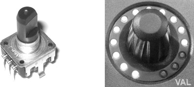
Figure 12.15 Two rotary encoders. The second is surrounded by an LED ring to indicate the current setting or position.
Rotary encoders rotate all the way around continuously, and are divided up into segments. They often have a clicky feeling to them when rotated, and each movement clockwise or counter-clockwise causes two switches to open and close indicating the movement. There is no way to know what the current position of a rotary encoder is – instead a microcontroller is typically used to count how many clicks left or right it has been turned.
They are useful as rotation sensors or selectors in digital systems, and are particularly handy because effectively they can be automatically reset and adjusted by the system. Many rotary encoders will include a ring of LEDs which are used to give a visual indication of their current setting. Rotary encoders will very often be encountered on digital sound desks and control surfaces.
Photoresistors
A component which can be used to great creative effect in audio electronics is the photo-resistor, light dependant resistor, or LDR. Figure 12.16 shows what they look like. The characteristic pattern snaking across the top of the device is the light sensitive region. As more light shines on the device this region becomes more and more conductive, reducing the resistance present between the two leads.
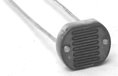
Figure 12.16 A light dependant resistor or photoresistor.
As with a number of circuit symbols, arrows at an angle indicate light. Here arrows arriving at a standard resistor symbol (Figure 12.17) indicate light sensitivity. Similarly, arrows departing at an angle can indicate light production, as is seen with the light emitting diode later.

Thermistors
Less common, but worth mentioning in this chapter about resistors is the thermistor or temperature dependant resistor, see Figure 12.18. Thermistors come in two types depending on whether their resistance rises or falls as their temperature rises. Positive temperature coefficient or PTC thermistors exhibit a rise in resistance with rising temperature. With negative temperature coefficient (NTC) thermistors the effect is reversed with resistance falling as the temperature rises.
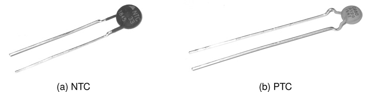
Figure 12.18 A negative temperature coefficient (NTC) thermistor and a positive temperature coefficient (PTC) thermistor.
Thermistors are often used in power amplifiers and other high power circuits to monitor the operating temperature of critical parts and activate some kind of safety circuitry if the temperature rises above a given threshold. They can also be used in so called soft start circuitry to limit current flow until the circuit has had a chance to get going. They are indicated on circuit diagrams using the symbols shown in Figure 12.19. The type (NTC or PTC) will often be indicated by two little arrows. Both arrows up indicates PTC, while one up and one down indicates NTC.
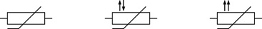
Figure 12.19 Thermistor symbols (unspecified, NTC, and PTC versions).
Instructive Examples
To help cement an understanding of the role resistance plays in electronic circuits, the following sections describe the structure and function of a number of commonly encountered subcircuits in which resistors play a pivotal role.
Generating a Reference Voltage
Audio circuits often operate from a power supply providing two rails. For instance the two terminals of a standard 9V battery might be connected to provide two power rails, labelled plus and minus, power and ground, +9V and 0V, or some similar designations. It is often necessary to derive an intermediate reference voltage at for instance 4.5V to supply key points in the circuit. This can be achieved using a simple voltage divider composed of two equal value resistors (Figure 12.20). Using the Voltage Divider Rule described earlier in this chapter, it is easily confirmed that the point marked Vref in this figure will sit at a voltage of four point five volts. In fact any pair of equal size resistors will, as can be seen from the equation, yield the same result.
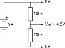
Figure 12.20 Voltage reference derived from a pair of equal resistors.
This approach to generating a voltage reference while useful does have some limitations. In isolation the subcircuit shown in Figure 12.20 will indeed provide a voltage at the point marked Vref which is half way between the voltages at its top and bottom. However when this reference voltage is used by connecting it to some point in a larger circuit the circuit to which it is connected can easily pull the voltage up or down or even cause it to swing back and forth constantly as the circuit operates.
In order to use this kind of simple voltage reference to provide a stable and well defined bias voltage in a circuit it is essential that the place or places to which it is connected in the circuit present a high impedance. This will make sure that they have a minimal effect on the level of the voltage reference which they are using. The commonest place this kind of simple voltage reference is encountered is connected to the input of an opamp as illustrated in Figure 12.21. Opamp inputs are generally designed to have a very high input impedance. As such they will draw minimal current and thus have as little an effect on the reference voltage as possible.
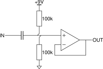
Figure 12.21 Typical circuit employing a voltage divider based reference voltage.
As stated above, in order to provide a voltage which is half way between the top and bottom voltages, the two resistors in the voltage divider must be of equal size. (Other voltage references can be generated using two non-equal sized resistors.) In Figure 12.20 and Figure 12.21 the resistors are shown as being 100kΩ each, and this is a value commonly used in this application. The value chosen is a compromise. The two resistors provide a direct path from power to ground and as such current will flow through them continually. Smaller values (less than perhaps 10kΩ) will place an unacceptable load on the circuit’s power supply (the 9V battery would be drained too quickly and would need to be regularly replaced). Conversely too large a value would result in a less stable reference as the circuit to which it is connected will have a greater impact on its value. These two opposing factors lead to the commonly encountered values between about 10kΩ and 100kΩ.
The other two components can be ignored for now. They are a capacitor and an opamp, and their roles in the circuit fragment shown here becomes clear in later chapters. Another capacitor will often be seen connected between Vref and ground in this kind of voltage reference subcircuit. One of the roles of a capacitor is to store charge and in this case a large (perhaps 10µF or larger) capacitor provides a little current reservoir which will help to stabilise the reference voltage and prevent the action of the circuit to which it is connected from moving it about too much. This capacitor while not shown here is a fairly common feature in this kind of voltage reference subcircuit and helps to minimise the unwanted voltage swings described above.
Attenuators and Volume Controls
If an audio signal is applied to the top of a voltage divider then what appears at the midpoint of the voltage divider is a smaller version of the same signal (Figure 12.22). How much smaller this signal is than the original is controlled by the relative sizes of the two resistors forming the voltage divider. This arrangement as illustrated in Figure 12.22a is often referred to as an attenuator or pad and it simply reduces the level of the incoming signal by a set amount. Once again, the Voltage Divider Rule can be used to determine the amount of attenuation in any given case.
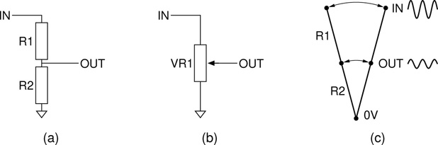
Figure 12.22 Voltage divider reducing the level of an incoming signal.
What is shown in Figure 12.22b is not a pair of fixed resistors as found in a pad but rather it is a pot or variable resistor. This can however be analysed in exactly the same way. A pot can be thought of as a simple voltage divider where the relative sizes of the two resistors vary as the pot knob is turned. As one gets larger the other gets smaller but the sum of the two always remains the same.
Imagine the arrow of the pot symbol moving up and down along the length of the rectangle as the pot knob is turned. The rectangle remains the same length but sometimes more of it is above the arrow and sometimes more of it is below the arrow. So for example, when the arrow is at the bottom, R1 in the voltage divider equals the total pot resistance and R2 equals zero. Putting these values into the Voltage Divider Rule indicates that Vout = 0.
Conversely when the arrow is at the top, R1 in the voltage divider equals zero and R2 equals the total pot resistance. Putting these values into the Voltage Divider Rule indicates that in this case Vout = Vin, maximum volume.
As the pot knob is turned the arrow can be thought of as moving between top and bottom, and Vout the output voltage or volume changes correspondingly between maximum (Vin) and minimum (0V).
Limiting Current Draw
By definition limiting current is what a resistor does. There are a couple of commonly encountered situations where this particular aspect of its action come to the fore. Sometimes a resistor is placed between the power supply and the rest of the circuit (Figure 12.23). This has the effect of reducing the overall current drawn by the circuit and thus extending the battery life. If the circuit in question does not need the full voltage available from the power supply this is a simple way of limiting current draw and extending battery life. In fact, this technique is sometimes employed more for the effect it has on the sound than for simple power control. An audio circuit can behave in different ways as the power supply is altered. Voltage droop is a recognised effect in some circumstances.

Figure 12.23 Resistor limiting current drawn from power supply.
This is certainly a crude approach to limiting the amount of current which is drawn by a circuit but can be quite useful. Some good examples of this technique in action can be found in the circuit ideas compiled by Tim Escobedo collected under the title ‘Circuit Snippets’ and readily available on the internet. (A number of the circuit ideas explored in this book can trace their origins to the ‘Circuit Snippets’ collection and anyone interested in exploring audio electronics will find something of interest in it.)
The current limiting action of a resistor is also employed in a very direct way when adding an LED to a circuit. LEDs require a specific amount of current in order to light up to their intended brightness. This current is usually controlled by a resistor as shown in Figure 12.24. Not enough current and the LED will be very dim while too much current will burn it out. The correct size of resistor must be chosen in order to allow the LED to operate correctly. This application is examined in more detail when LEDs are discussed in Chapter 16.
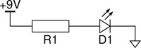
Figure 12.24 Resistor controlling current to LED.
In the examples above, the details of how much the resistor will limit the current depend on the rest of the circuit as well as the current limiting resistor itself. It is however a simple matter to determine the maximum current draw of the system, based on the value of the resistor used, along with the supply voltage. Suppose R1 is 330 in either of the above examples. Recalling Ohm’s law from Chapter 9, the required calculation becomes clear.
Similarly, if R1 is increased to 1kΩ, the maximum possible current draw is reduced to 9/1,000 = 9mA. If the impedance of the rest of the circuit is low then this limit set by the resistor will be approached. As the impedance of the rest of the circuit rises, the actual current draw drops off accordingly.
References
G. Ballou. Resistors, capacitors, and inductors. In G. Ballou, editor, Handbook for Sound Engineers, ch. 10, pp. 241–272. Focal Press, 4th edition, 2008.
D. Bohn. RaneNote 149: Interfacing AES3 & S/PDIF. Rane Corporation, 2009.
D. Self. Small Signal Audio Design. Focal Press, 2nd edition, 2015.