13 | Capacitors and Inductors
Capacitors and inductors are examined together because these two components are very closely related, despite being markedly different in structure and operation. At the very simplest level a capacitor is composed of two sheets of conductive material separated by a layer of insulating material, while an inductor is nothing more than a length of wire wound into a coil. The relationship between capacitors and inductors stems from their very differences. While not holding in all cases, there is a symmetry between these two components. As a general rule whatever one does the other is likely to do the exact opposite. This is illustrated in the one line descriptions for each component, highlighted in the box above; capacitors block low frequencies and pass high frequencies, while inductors exhibit the opposite behaviour passing low frequencies and blocking high frequencies. Often this is as much information as is needed in order to see what role a capacitor or inductor plays in a particular circuit, although capacitors in particular are used to do a great many useful things in audio electronics.
Capacitors
After resistors, capacitors are the most commonly encountered component in typical audio electronic circuitry. Capacitors can also be said to exhibit what from many perspectives is the widest variety of different types and subtypes of any electronic component. Where for instance resistors are most often of either carbon film, metal film, or sometimes wire wound construction, and transistors usually appear in the form of either BJTs or FETs with a few variations of each, capacitors come in a wide array of forms and formats the full range of which is only touched upon in this chapter. The range of shapes, sizes, and types provides for a rich area of experimentation in audio circuits as the sometimes subtle differences in the performance of different types can result in slight but sometimes audibly significant variations in their effect.
A variety of circuit diagram symbols can also be encountered representing capacitors, the most standard of which are illustrated in Figure 13.1. Quite a few variations on these symbols are found but they are all pretty similar, and on the whole fairly self explanatory. Watch out for polar or polarised capacitors (most often electrolytic or sometimes less common tantalum types). Polarised capacitors must be inserted into a circuit the correct way round. They should not be used in positions where the polarity of the applied voltage is expected to reverse in normal operation. Most often polarised capacitors are indicated in a circuit diagram by a symbol with a plus sign on one side of the component as in Figure 13.1b. Occasionally a different symbol with one straight and one curved line is used, and other variations are also encountered, the most common of which are included in the schematic symbol reference chart in Appendix C.
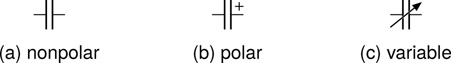
Figure 13.1 Circuit diagram symbols for a capacitor.
The units used to measure the capacitance value of a capacitor are called farads (F). However one farad represents an very large device (they do exist but are unlikely to be encountered in audio electronics). Commonly used capacitors will have values measured in microfarads (µF, often pronounced ‘mike’), nanofarads (nF), and picofarads (pF, often pronounced ‘puff’). Micro- means divided by a million, nano- divided by a billion, and pico- divided by a trillion. See Appendix A for a full explanation of all the multiplier prefixes which are likely to be encountered working in audio electronics.
When considering the division of capacitors into polar and nonpolar types, as a rule of thumb capacitors smaller than about one microfarad (1µF) will typically be nonpolar types while above this size they will most often be of polar construction. If a polar type is specified in a design it will usually be fine to substitute a nonpolar type of the same size if one is available. Substituting a polar where a nonpolar had been specified is less likely to work satisfactorily.
Capacitor Types
As previously noted the capacitor is probably second to none in the variety of device types and subtypes available. Table 13.1 only scratches the surface of the wide range of component types which can be encountered but it does highlight what are probably both the most common and most important variants utilised in modern audio electronics along with some of the key characteristics which define their operation and use.
Table 13.1 Common capacitor types and typical values for various important characteristics
Ceramic |
Film |
Electrolytic |
Tantalum |
|
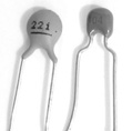
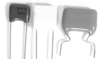
Examples |
|
|
|
|
Subtypes |
NP0/C0G, X7R, Z5U, Y5V |
Polyester, Polypropylene, Polystyrene... |
Polar, Nonpolar/Bipolar |
Dry slug, Wet slug |
Typical ranges and values for small signal devices – |
||||
Capacitance |
10pF to 220nF |
1nF to 1µF |
1µF to 1000µF |
100nF to 63µF |
Tolerance |
±10% |
±5% to ±10% |
±20% |
±20% |
Voltage |
63V/100V |
100V |
25V/50V |
3V to 35V |
For the most part, all these names and designators indicate the nature of the dielectric employed in the construction of the device. The dielectric is the insulating layer which separates the two conductive plates of a capacitor and its precise composition can dramatically affect the performance of a component. As illustrated in Table 13.1 some dielectric types are best used for manufacturing only a limited subset of the wide range of capacitance values encountered. Some types need to be made physically very large in order to achieve larger capacitance values. Higher voltage ratings also result in physically larger devices and some dielectrics will not tolerate high voltages in any case. Size can be an issue as it is often necessary to make circuitry as small as possible when designing and building audio (and other) equipment.
The precise types employed can be of great importance when designing high quality, low noise (and expensive) audio equipment but are generally of lesser importance in the applications under consideration in this book. Amongst the ceramic types the NP0 subtype (aka C0G) is an excellent part which compared to other ceramic subtypes introduces minimal distortion into applied audio signals. Similarly in the range of film subtypes polypropylene or PP devices usually demonstrate superior performance to the more commonly encountered polyester or other film subtypes used in audio applications (Self, 2015, pp. 63–74). Needless to say, in both cases this enhanced performance usually comes at a significantly higher cost and the amount of improvement achieved is typically neither justified nor required in nonspecialist applications.
Typical capacitance values commonly encountered range from a few picofarads up to a few hundred microfarads. Different types tend to cover different ranges as shown in Table 13.1. As a rough guide ceramics cover the low end, film types range through the middle of the spectrum, and electrolytics are usually employed for larger values. Tantalum capacitors which tend to be available in mid to high values are usually considered to be somewhat specialist parts. In audio applications their use can be a hot topic for debate on various audio electronics forums. They probably introduce more distortion than other types but the question of whether it is good or bad distortion is a matter of subjective preference. They can provide a large capacitance in a small package.
It is important to observe the voltage ratings of capacitors, which can sometimes be quite low. For a circuit powered by 9V (as most examined here are) it is probably wise to stay above about 16V or 18V ratings for the capacitors used. This should not be an issue except for some tantalum types (it is also worth remembering that tantalum capacitors are very easily damaged by even small reverse voltages, remember they are a polarised type). When looking at a high wattage power amplifier or similar where much higher voltages can be involved then more attention needs to be paid to the voltage ratings of the capacitors used. Again commonly encountered voltage ratings vary from type to type and typical values are indicated in Table 13.1.
Capacitor tolerances tend to be quite wide with ±20% or more not being uncommon especially for electrolytics. The somewhat more expensive polypropylene capacitors often have a somewhat more respectable ±5% rating or better. Generally this is not an issue. In many circuits the precise values of the capacitors used are not critical to their operation, or the variations encountered can be compensated for in other ways.
Capacitor Applications
As previously stated capacitors block low frequencies and pass high frequencies. This makes them of particular interest in audio electronics as the manipulation of an audio signal’s frequency spectrum is a fundamental tool in the design of useful audio circuits. In fact capacitors play a number of key roles in the operation of typical audio circuitry. To give a flavour of the wide gamut of uses where capacitors are employed Table 13.2 highlights some of their more important areas of application.
Application |
Description |
Blocking and coupling |
Capacitors are often used to remove DC and/or subsonic, low frequency components from a signal while coupling the main audio frequencies through to the next part of the circuit. |
Filtering |
Capacitors are a fundamental part of filter and EQ circuits designed to cut or boost various sections of the audio frequency spectrum in a signal. |
Smoothing and storing |
Capacitors can be used to adsorb ripple, noise, and interference on a circuit’s power lines, and to provide short bursts of high current when signal levels peak. |
Suppressing and decoupling |
Capacitors can be used in many circuits to attenuate or suppress unwanted signals such as high frequency circuit resonances and RF (radio frequency) interference. |
Timing |
Capacitors are often used in conjunction with resistors to set the frequency of oscillation in various signal generator and oscillator type circuits. |
Inductors
As explained at the beginning of this chapter, an inductor is just a coil of wire. Its impedance rises as frequency rises. Inductors are used only quite rarely in audio circuits. They tend to be bulky, expensive, and nonlinear. In most aspects of their behaviour they are the exact opposite of capacitors, so most things which can be achieved with inductors can also be done with capacitors, by reconfiguring the circuit in some fashion. Most of the circuit symbols commonly used to represent inductors reflect their structure well, consisting of either a spiral or a series of loops as shown in Figure 13.2. See Appendix C for some additional symbols also commonly encountered.

Figure 13.2 Circuit diagram symbols for an inductor.
The variations shown in Figure 13.2 also reflect the fact that an inductor’s performance can be significantly altered depending on the nature of the core around which the coil is wound. As indicated, the three commonest methods of construction involve an air core (i.e. no core at all), a solid or laminated metal core, or a ferrite core. Ferrite cores are made from iron dust or filings mixed with a binding agent and moulded into the required shape. An inductor’s core material strongly influences its size and performance (much like the dielectric material in a given capacitor).
In many cases inductors are easily recognisable since the coil is often clearly visible, as in the examples in Figure 13.3, although sometimes they are encased inside a plastic casing or a metal can. Some smaller inductors look very similar to standard through hole resistors.
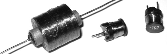
Figure 13.3 Some typical inductors.
The unit of measure for inductors is the henry (H). Most commonly encountered inductors will have values in the millihenry (mH) range with some falling to the level of microhenries (µH). Inductors are on the whole far less commonly employed than capacitors, but there are a few interesting audio circuits which call for an inductor, often being used in some form of a filter or EQ role. Many classic wah pedals (such as the much loved Dunlop Cry Baby) use an inductor in the design of their swept filter. An interesting filter design, combining inductors and capacitors, may be heard generating the characteristic washed out high pass filter sound used to great effect by some early reggae producers. One example of this is what came to be referred to as ‘King Tubby’s big knob filter’ on account of the larger than standard pot knob used to control this particular filter on his mixing desk (Williams, 2012).
RF Chokes and Noise Suppression
One very common source of interference and unwanted noise in electronic circuits is through the pickup of radio frequency (RF) signals from the air. With the stated primary behaviour of an inductor bing that it passes low frequencies and blocks high frequencies, it would seem reasonable to suggest that the inductor might prove an effective tool in the suppression of unwanted RF interference in audio signals, and this is indeed the case. Figure 13.4 illustrates a number of RF choke cores moulded from ferrite material.
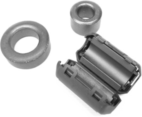
Figure 13.4 Ferrite cores for use as RF chokes.
The third in particular (in a hinged plastic case) can commonly be found around the power leads and signal connectors of many electronic devices where it acts as a block to any high frequency signal which tries to pass it. Low frequency signals, and the DC power signals which it is often found working in conjunction with, can pass freely along the wire to which such an RF choke is applied. It may not be immediately obvious where the inductor is in this case. In fact it is formed by the cable itself, running through the ferrite core. Sometimes the cable is looped back to perform a second pass through the core and thus increase the inductance induced, but often simply passing the cable through a core formed tightly around it is sufficient to achieve the high frequency filtering desired.
Characteristics of Capacitors and Inductors
Many of the details of component characteristics examined in the previous chapter on resistors apply equally to capacitors and inductors. These aspects of a component’s performance are mentioned only briefly here. For more details on the interpretation and use of these parameters refer back to the appropriate sections of Chapter 12. Table 13.1 shows typical values for the most important capacitor characteristics. Inductors generally display less variation in their available types and variants.
Preferred values – the same E-series preferred values which are used to specify standard resistances also generally apply to capacitors and inductors. Fewer values are typically available, with E6 or even E3 being very commonly offered ranges.
Tolerance – the more limited range of values typically available reflects the fact that capacitors and inductors tend to be manufactured to much looser tolerances then resistors. They are usually specified as ±10% or even ±20% as compared to typical resistor tolerances of ±1% and ±5%. Tighter tolerance capacitors are available but quickly become prohibitively expensive and are unnecessary for all but the most demanding applications. Tighter tolerances in inductors are rare but not unheard of. In most cases circuits can be designed to provide the desired levels of performance without having to resort to these more expensive parts.
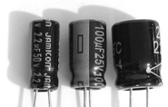
Markings – while a very few capacitors can still be found which use a colour code similar to resistors in order to display their nominal value most capacitors will have their values printed on them. The value is likely to be formatted in one of two ways. On electrolytic capacitors and other physically large devices it is often printed directly (e.g. 470µF). On other types (which tend to be physically smaller) a simple three digit code is usually used. The first two digits indicate how the value starts and the third indicates how many zeros to add to complete the value given in picofarads. So for example 224 means twenty two followed by four zeros, 220,000pF, two hundred and twenty thousand picofarads, or two hundred and twenty nanofarads.
Polarised capacitors use a couple of different marking methods to differentiate the positive and negative terminals. Electrolytic types will usually have a row of minus signs running towards the negative leg. Tantalum capacitors on the other hand tend to mark the positive pin with a plus sign. Some older tantalum types used a colour code with a number of horizontal stripes and a single blob or dot of colour. For these types the rule ‘when the dot’s in sight the positive’s on the right’ was used to identify which way round they were to be connected.
Inductors can be commonly encountered using either a colour code or a printed value. Typical values span the micro- and millihenry ranges. The smallest devices can range into the nanohenry region while larger values extend up to several henries.
Voltage rating – a key characteristic of a capacitor is its voltage rating. It holds a similar position to the power rating parameter described for resistors. This is the maximum voltage which the capacitor should ever to exposed to and sometimes these values can be quite low so it is worth keeping an eye on this value when using capacitors. It will often be printed on the body of a capacitor along with the capacitance value.
Current rating – for inductors the corresponding parameter to a capacitor’s voltage rating or a resistor’s power rating is the current rating most often specified as a DC current rating. Since inductors pass low frequencies and block high frequencies they pass DC (i.e. 0Hz, the lowest possible frequency) best of all. This means that a DC voltage can overload and burn out an inductor very easily by causing a large current to flow through it. An inductor circuit must be designed to ensure that excessive currents are not allowed to flow through the inductor in normal operation.
As with resistors many other parameters and specifications exist covering all aspects of the construction and behaviour of various devices. In the main these details can be ignored in all but the most demanding of applications.
Device Impedance
The impedance of a device measured in ohms (Ω) indicates how easily or with what level of difficulty electricity will flow through that device. Resistors as described in the previous chapter have a resistance (also measured in ohms) which is pretty much constant across the full range of the devices operating conditions. Resistance is just one component of impedance. When capacitors and inductors enter the scene the other side of impedance is encountered. This second component is called reactance. Together resistance and reactance make up impedance. Resistance can be considered as the constant part of impedance while the reactive portion of impedance changes depending on the frequency of the electricity flowing through the component in question.
So resistors have a reactance of zero. Their impedance is purely resistive and so it doesn’t change with frequency. On the other hand capacitors and inductors generally have zero (or negligible) resistance but non-zero reactance meaning that their impedance varies as the frequency of the signal passing through them varies. Eq. 13.1 shows how to calculate a capacitor’s impedance. Note that just as R has been used previously to indicate resistance in equations, X is now employed to indicate reactance, XC for capacitive reactance and XL for inductive reactance. Later when resistance and reactance are combined, Z will appear to indicate total impedance as a function of these others. These are the standard letters used to indicate these quantities in equations. All of these quantities are measured in ohms (Ω).
As can be seen from Eq. 13.1 the value of a capacitor’s reactance depends on the capacitance of the device and the frequency of the signal. So for a given device which has a fixed value (measured in farads) the impedance can be plotted against the frequency of the signal applied. This relationship is graphed in Figure 13.5 for three capacitance values: 22nF, 47nF, and 100nF. As the frequency increases the impedance decreases. This illustrates the capacitor’s core behaviour which clearly explains why capacitors block low frequencies and pass high frequencies. At low frequencies the impedance becomes very high and so little signal can get past while at high frequencies the impedance becomes very low and so signals have little difficulty in passing through.
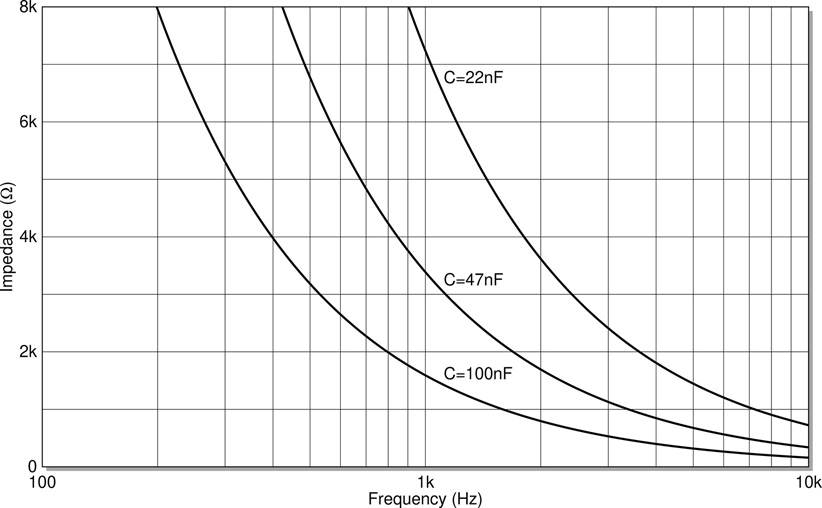
Figure 13.5 Graph of capacitor impedance plotted against frequency.
As has been pointed out previously capacitors and inductors behave in broadly opposite fashions, and so it should be no surprise to see the form of the impedance equation for an inductor as shown in Eq. 13.2. Instead of getting smaller as the frequency grows larger, the inductor’s impedance increases along with the frequency. L is the letter conventionally used to indicate inductance in equations just as C is used to represent capacitance.
In Figure 13.6 the behaviours of resistor, capacitor, and inductor are plotted on the same graph in order to highlight their relationships and their differences. The resistor plot consists of a horizontal line indicating that the impedance remains at the same level at all frequencies. As the value of the resistor is changed the horizontal line will appear higher or lower on the graph. So the plot for a 8kΩ resistor would be a horizontal line crossing high up on the graph while that for a 100Ω resistor would appear still horizontal but much lower down.
The curves to illustrate capacitors of differing values would move either towards or away from the origin of the graph depending on the size of the capacitor as is well illustrated by the three plots in Figure 13.5. Larger capacitor values correspond to plots which traverse ever closer to the origin while smaller value capacitors result in plots lying farther out.
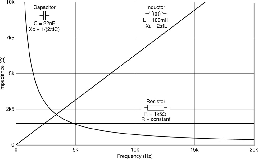
Figure 13.6 Graph of resistor, capacitor, and inductor impedance versus frequency.
It is worth noting that the same information is sometimes plotted using log scales on the Impedance and Frequency axes. This type of rendering results in straight lines instead of curves for the capacitor plots as illustrated in Figure 13.7. It is important to realise that these two representations are entirely equivalent. No new or different information is being displayed by this seemingly different graph. It is just another way of plotting the same impedance functions shown above. The lines for resistance and inductive reactance remain straight lines. Notice that in this second style of plotting the origin of the graph (0,0) will never appear. Moving down and to the left the numbers get smaller and smaller but they never reach zero. This helps to explain how a curved line in the previous plot which gets closer and closer to but never touches zero lines of the X and Y axes can become a straight line in this one.
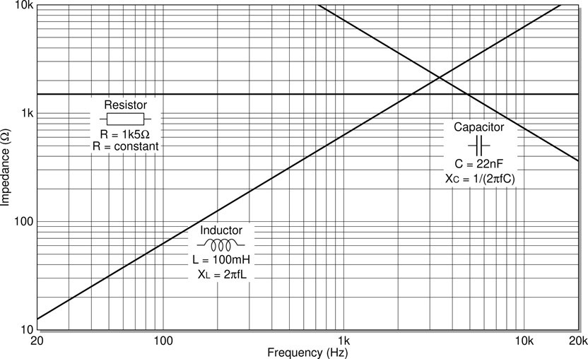
Figure 13.7 Graph of resistor, capacitor, and inductor impedance using log scales.
The third line in Figure 13.6 and Figure 13.7 plotting an inductor’s reactance (Eq. 13.2) is a straight line through the origin. This means that when the signal frequency is zero the inductor reactance is zero which can be seen from the inductor’s impedance equation. Once again this matches with the key characteristic of inductors that they pass low frequencies and block high frequencies since a low impedance will pass a signal and a high impedance will block it.
Inductors of different values result in straight lines of different slopes all passing through the origin. As the inductance is increased the reactance at any given frequency also increases so larger inductances result in lines of greater slope becoming increasingly close to the vertical and smaller inductances result in shallower slopes becoming increasingly close to horizontal.
Notice that the three previous figures all use different combinations of linear and logarithmic scales for their axes even though they are all plotting the same information on each axis, frequency on the X axis and impedance on the Y axis. The use and interpretation of these different graphing scales is more fully examined in Chapter 5 where the four possible combinations of linear and logarithmic scales are examined, along with their relationship to the decibel scale.
Equivalent Series Resistance
The simple ideal models of component behaviour are often sufficient, but they never tell the whole story. For example a real capacitor will exhibit resistance and inductance as well as capacitance. The levels of inductance present are so small that they only become a concern at very high frequencies well beyond the audio. Some capacitors, particularly electrolytics, do however present a small but sometimes significant resistance. This is called ESR or equivalent series resistance.
Generally in film and ceramic types it is small enough to ignore, typically well less than an ohm, but in electrolytics it is often as much as a few tens of ohms. Low ESR is important because the lower the ESR the faster the capacitor can charge and discharge. This is a great benefit because it means that such capacitors can respond faster to large transients. Resistance also means power dissipation.
Sometimes a small ceramic capacitor is used in parallel with a much larger electrolytic capacitor. At first glance it would seem to have little effect on the circuit as it adds just a small bit more capacitance to the large amount already provided by the electrolytic. However at high frequencies the electrolytic’s relatively large ERS degrades its performance and the ceramic with its much smaller ERS is able to step in. This arrangement is often seen where digital ICs need decoupling to prevent noise glitches generated by fast switching digital circuitry from contaminating the power supply.
Eq. 13.7 and Eq. 13.8 in the section on RLC circuits which follows are presented in terms of analysing circuits which combine actual capacitors, inductors, and resistors. However they can also be applied here to more accurately calculate a component’s true impedance by combining its resistive and reactive elements. This is seldom if ever required in the kind of circuit analysis needed here but it is worth bearing in mind.
Series and Parallel Rules
Rules are introduced in Chapter 12 to calculate the effect of series and parallel combinations of resistors. The same configurations can also be very useful when applied to capacitors and inductors. This can be particularly the case because the values readily available for capacitors and inductors are often far more limited than those available for resistors and so it is often necessary to make up a value required in a particular circuit by combining two or more components of those values which are available.
The four equations given here for series and parallel combinations of capacitors and inductors follow the same pattern as the earlier equations given for resistors. It should be noted however that when compared to the resistor case the two equations for capacitors are reversed while they remain in the original order for inductors. In other words for straight addition of values resistors and inductors are places in series but capacitors are placed in parallel.
It is always the case that one configuration will give a resultant value larger than either of the constituent components while the other configuration gives a resultant value smaller than either on its own. Resistances and inductances get bigger in series and smaller in parallel while capacitances get smaller in series and bigger in parallel.
|
(13.3) |
|
|
(13.4) |
|
|
(13.5) |
|
|
(13.6) |

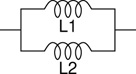
Combining three or more components in series or parallel is simply a matter of multiple applications of the rules provided here. Indeed any network composed solely of one of these three types of components resistors, capacitors, or inductors no matter how large and complex can be simplified down into a single value which can then be used in analysing the behaviour of the original network. Figure 13.8 shows a (somewhat unlikely) network of inductors. The steps below illustrate one way to go about determining the overall inductance of the network. A number of alternative routes through such a process will often exist but they will always yield the same final result. In this case for instance step one might either be to combine L1 and L2 or alternatively L3 and L4 might be combined first and so on. At each stage it is necessary to identify two components which can be combined into one through the application of either the series or parallel rule. Ultimately the entire network is replaced by a single component value.
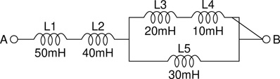
Figure 13.8 Example inductor network.
Step 1: Combine L1 and L2, series rule – Lx = L1 + L2 = 50m + 40m = 90mH
Step 2: Combine L3 and L4, series rule – Ly = L3 + L4 = 20m + 10m = 30mH
Step 3: Combine Ly and L5, parallel rule
Step 4: Combine Lx and Lz, series rule – Ltotal = Lx + Lz = 90m + 15m = 105mH
And so the total inductance between points A and B through the inductor network shown in Figure 13.8 is equal to 105mH, one hundred and five millihenries. The same procedure can be applied to resolving any R, L, or C network into a single equivalent value for the purposes of analysis.
RLC Circuits
Up to this point each type of component has been considered in isolation being combined only with other components of its own type. Some very useful circuits (for example simple low pass and high pass filters) can be constructed by combining resistors (R), inductors (L), and capacitors (C). Circuits involving any combination of these three components are traditionally referred to using the corresponding letters, so that for instance an LC circuit is composed solely of inductors and capacitors, and so forth.
In order to understand the operation of such circuits a number of additional equations are needed, describing how the different components combine and interact. A full analysis would include consideration of the effect on the phase of signals of different frequencies passing through such combinations of components. This kind of analysis is more advanced than is required here. In this work only the magnitude component is considered.a
Previously Eq. 13.1 and Eq. 13.2 showed how to calculate the impedance of a capacitor or inductor at a given frequency (recall that unlike resistors, capacitor and inductor impedances are frequency dependent). The next step which must be taken is to calculate the frequency dependant impedance of a circuit consisting of different component types in series or parallel. Eq. 13.7 and Eq. 13.8 show how such impedances can be determined.
|
(13.7) |
|
|
(13.8) |
These equations can be used for RL, RC, and LC circuits by simply dropping the unused term in the appropriate equation. If R is dropped the simplified forms in Eq. 13.9 and Eq. 13.10 can be derived. It should be quite straightforward to see that Eq. 13.9 can be arrived at by setting the value of R in Eq. 13.7 to zero, and similarly Eq. 13.10 can be arrived at by setting the value of R in Eq. 13.8 to infinity (i.e. an open circuit in parallel with the two other components). Eq. 13.9 and Eq. 13.10 are given as simplifications of Eq. 13.7 and Eq. 13.8 because these cases where capacitance and inductance but no (significant) resistance are present are quite common and the associated equations are thus correspondingly useful.
_________________________
|
(13.9) |
|
|
(13.10) |
Notice that in all four equations the capacitive and inductive reactances are subtracted not added. This might seem counterintuitive at first but is in fact the case and again reflects the equal but opposite natures which have previously been pointed out as existing between capacitors and inductors. In the first two equations the square eliminates any possible negative answer resulting from this subtraction while in the second pair the magnitude operator arrives more simply at the same result as square followed by square root. As a result these equations always yield a strictly nonnegative impedance as is to be expected from a magnitude calculation.
RLC Time Constants
One common use for capacitors is in setting the time constant of a circuit. A time constant might be used to control the frequency of oscillation of an oscillator circuit or the attack and release times in an envelope generator for instance. By extension inductors can be used in a similar fashion but this is much less common as the use of inductors is rare in general. As has been mentioned previously inductors have a few significant drawbacks (size, price, nonlinearity etc.) which generally make their use much less appealing then capacitors in most applications.
The idea of the time constant is that when a capacitor is charged through a resistor the voltage across the terminals of the capacitor rises in a very well defined and predictable way. Consider the circuit shown in Figure 13.9. Initially the switch is in position A and the voltage across the capacitor is zero. As soon as the switch is moved to position B current starts to flow through the resistor and the voltage across the capacitor begins to rise. The manner in which the voltage rises over time is plotted in the graph in Figure 13.9. Initially a large current flows and the voltage rises rapidly but as the voltage across the capacitor rises the voltage remaining across the resistor must fall (KVL) and as such Ohm’s law means that the current flowing must fall. Eventually the capacitor is fully charged the entire available voltage is dropped across the capacitor and there is no voltage left across the resistor and hence no more current flows.
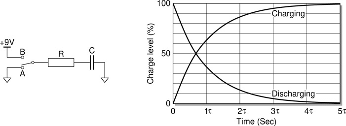
Figure 13.9 Circuit and graph for charging a capacitor through a resistor.
If the switch is at this point moved back from position B to position A the charging process is reversed and the capacitor is discharged through the resistor as per the second plot on the graph in Figure 13.9. The charge and discharge profiles are as illustrated in the graph logarithmic in nature starting off fast and then slowing down as they progress. The rate of charge or discharge can be characterised by the time constant.
Here τ (the lowercase Greek letter tau) represents the time constant and as before R is the size of the resistor in ohms and C is the size of the capacitor in farads. The time constant as defined above is the time it takes to charge the capacitor through the resistor to approximately 63% of the final voltage. This also equates to the time taken for it to fall to about 37% of the initial voltage in the case of discharging the capacitor (the charge and discharge curves are identical in shape mirrored around the horizontal). The actual functions which define the charge and discharge curves are rarely needed. They are simple exponentials and are included below for reference. In them t is time in seconds and the levels vary between zero and one. Multiplying by a hundred yields the percentages plotted in Figure 13.9.
vt = vfinal × (1 − e−t) |
− charging a capacitor or energising an inductor |
vt = vfinal × e−t |
− discharging a capacitor or deenergising an inductor |
Multiples of τ are often quoted when examining the behaviour of an RC circuit. It is usually taken that 5τ, having allowed the voltage to surpass 99% of the final value, is effectively the stopping point where steady state has been achieved. In other words the capacitor is then taken to be fully charged (or fully discharged as the case may be). See Table 13.3 for commonly used multiples of the time constant and what they translate to in terms of the degree of charging or discharging achieved in a circuit.
Table 13.3 Charge/discharge levels corresponding to various multiples of τ
Time |
% of maximum (charging) |
% of maximum (discharging) |
0.5τ |
39.3% |
60.7% |
0.7τ |
50.3% |
49.7% |
1.0τ |
63.2% |
36.8% |
2.0τ |
86.5% |
13.5% |
3.0τ |
95.0% |
5.0% |
4.0τ |
98.2% |
1.8% |
5.0τ |
99.3% |
0.7% |
Once again it should come as no surprise that a similar analysis is possible for a circuit where the capacitor is swapped for an inductor except that in this case instead of tracking the rise and fall of voltages it is the current flowing through the circuit which first rises to a maximum and then dies away to nothing as the switch is moved from A to B and then back again. In the case of an inductor the time constant τ is calculated as follows.
Again τ represents the time constant and as expected L is the inductance in henries and R is again the resistance in ohms. In this case τ is the time taken to energise inductor L through resistor R to 63% of its final current. Initially the current starts off slowly as the growing electric field opposes its flow but as the field is established and slows its rate of change more current is allowed to flow.
Passive Filters
A passive circuit involves only passive components such as resistors, capacitors, and inductors. An active circuit includes active elements like transistors and ICs, and requires a source of power in order to operate. Generally speaking amplification of a signal requires active circuitry. Passive circuits can cut the power level of a signal, but they can not boost it. Some passive circuits (most notably those involving transformers, as explored in the next chapter) can boost voltage at the expense of current or current at the expense of voltage, but the power in the signal is at best maintained at a constant level, or more likely drops. Only an active circuit can boost the power of a signal (by drawing power from a power supply). Recall from Watt’s law that power in watts is the product of voltage and current (P = I × V), and so it can be seen how voltage might be traded against current without any increase in power.
Filters are circuits designed to alter a signal’s frequency makeup by passing some frequencies and rejecting others. The most commonly encountered filter types are the familiar high pass filter (HPF) and low pass filter (LPF). Standard passive RC high pass and low pass filter circuits along with their respective frequency response characteristics, shown as graphs of signal attenuation measured in decibels plotted against frequency in hertz, are given in Figure 13.10 and Figure 13.11 below. Filters such as these are characterised in terms of their cutoff frequency. The formula for calculating the cutoff frequency in a standard RC filter is shown by Eq. 13.13. This relationship holds for both high pass and low pass RC filters. The cutoff frequency of any of the filter types described here is defined as the frequency at which the output level falls 3dB below the corresponding input level. This is often also referred to as the −3dB point or half power point.
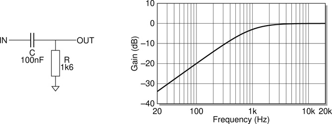
Figure 13.10 Simple RC high pass filter circuit and frequency response.

Figure 13.11 Simple RC low pass filter circuit and frequency response.
By substituting the expression for the RC time constant from Eq. 13.11 this equation can be rewritten as fc = 1/2πτ . It is instructive to note that this version of the equation also works in the case of the corresponding RL filters examined later as can be seen by combining Eq. 13.12 and Eq. 13.14. Notice from the frequency response graphs that these simple filter types do not cut off very quickly. The signal level, although falling all the time remains significant for quite some distance beyond the nominal cutoff frequency. More elaborate filter designs can achieve a faster rate of fall but for these basic types the rate of fall (referred to as the slope of the filter) is constant at a modest −6dB per octave.
The Passive High Pass RC Filter
The operation of the passive RC high pass filter as shown in Figure 13.10 is quite straightforward to decern from a basic examination of the circuit. Consider what happens to a low frequency signal component and a high frequency signal component arriving at IN. Recall that the fundamental action of a capacitor is that it blocks low frequencies and passes high frequencies. Thus the series RC arrangement present in this circuit acts as a frequency dependent voltage divider. For low frequencies the top impedance associated with the capacitor is very high and the voltage at OUT is pulled closer to ground by the relatively small resistance of R. As the frequency climbs higher the situation is reversed with the resistance of R now dominating thus sending OUT up towards the level present at IN.
A quick check can be performed using Eq. 13.13. Inserting the known values for R and C the expected cutoff frequency for the circuit shown can be calculated.
Looking to the accompanying graph, the cutoff frequency at −3dB can be seen to be very close to 1kHz confirming that roll off is commencing at the correct point. It is also noted that these simple RC filters should (once sufficiently beyond the knee) have a slope of −6dB per octave (or equivalently −20dB per decade, these two amount to the same thing). This slope can be confirmed using either of these metrics. Looking at the line from 20Hz to 200Hz (one decade) it can be seen to rise from about −34dB to about −14dB, a change of 20dB in one decade. Similarly at 100Hz the line crosses −20dB, and at 200Hz is again at about −14dB, thus a change of 6dB over one octave. These observations help to confirm the accuracy of the graph which is plotted in Figure 13.10.
The Passive Low Pass RC Filter
Since the specified component values in Figure 13.10 and Figure 13.11 are the same, the high pass and low pass cases shown are completely symmetrical, and so all the analysis performed up to this point also applies to the RC low pass filter in Figure 13.11 with the appropriate reversal of resistor and capacitor terms as needed. The cutoff frequency and slope are both unaltered, but in this case the graph falls with increasing rather than decreasing frequency.
RL High Pass and Low Pass Filters
As noted before, any circuit involving capacitors is likely to have a closely corresponding inductor based circuit. Figure 13.12 illustrates the equivalent RL based high pass and low pass filter circuits, corresponding to the RC circuits just presented, while Eq. 13.14 shows the RL form of the cutoff frequency equation.

Figure 13.12 RL high pass and low pass filter circuits.
The component values in these four high pass and low pass filter circuits are chosen to be commonly available values to give corner frequencies close to 1kHz. The two RC filters actually have cutoff frequencies at about 1019Hz, while the corresponding RL configurations lead to frequencies of approximately 995Hz. Given component tolerances and expected deviations from ideal performance these are quite close enough to be considered equal for most purposes. These values can be confirmed using Eq. 13.13 and Eq. 13.14.
Standard Filter Section Configurations
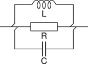
As alluded to above, the basic filter configurations presented so far are just the simplest of a large family of associated passive filter types. Analysis of the performance of these more elaborate variants gets very mathematical very quickly, and is not pursued further here. For the reader who wishes to get deeper into filter design many good references exist (e.g. Niewiadomski, 1989; Williams and Taylor, 2006). Some of the more commonly encountered configurations are illustrated in the figures below.
Figure 13.13 shows the basic configuration already examined (referred to as an ‘L’ section), alongside two variations on the theme referred to as ‘T’ section and ‘Π’ section configurations respectively. All three filter sections shown here implement high pass filters. Unsurprisingly, any of the three can be converted to a low pass filter simply by swapping resistors and capacitors. These various configurations are often encountered in audio circuits.
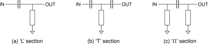
Figure 13.13 Standard filter section types.
Figure 13.14a shows the twin-T configuration. It should be clear that this is an HPF and an LPF wired in parallel. The result is a band stop filter or notch filter. The LPF half allows frequencies below the notch to pass, while the HPF half allows frequencies above the notch through. The labelling given here represents the commonest, and simplest, arrangement, where the capacitor to ground (labelled 2C) is twice the size of the other two capacitors, and similarly the resistor to ground (labelled R/2) is half the size of the other two resistors.
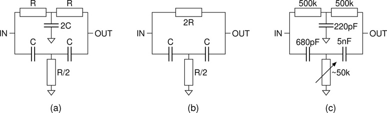
Figure 13.14 The twin-T and bridged-T filter configurations.
Figure 13.14b shows a simplification of the twin-T which is occasionally encountered, called the bridged-T configuration. The capacitor to ground is dropped, and as a result the two resistors labelled R, now being simply in series, can be replaced by a single resistor of twice the size (2R).
Finally, Figure 13.14c shows a variation on the standard twin-T with non-matching component values selected. This example is another taken from the ‘Circuit Snippets’ collection; the circuit in question is called the ‘Idiot Wah’, and the twin-T implements the standard wah swept notch filter. The variable resistor on the lower ‘T’ represents the effects familiar foot pedal control.
As noted in the comments accompanying the ‘Idiot Wah’ circuit from which the shown values are taken, ‘the unequal capacitors in the T network give a more useful, more musical range than the typical matched values’. These observations will of course be a matter of individual taste, but as always the general rule is, experiment. The original circuit as found in the ‘Circuit Snippets’ collection also includes a switch on the 220pF capacitor to ground, allowing the twin-T to be converted into a bridged-T configuration as in Figure 13.14b, for added sonic possibilities.
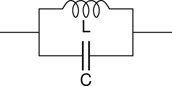
LC Filters
So far all the filters presented have involved a combination of resistor and either capacitor or inductor. Another common variation is to drop the resistor and just combine capacitors and inductors. Figure 13.15 illustrates basic high pass, low pass, and band pass LC filters. LC filters have advantages and drawbacks when compared to their RC and RL cousins. They avoid the inevitable insertion loss of a resistance based filter; a resistor must drop voltage and dissipate power at all frequencies, whereas capacitors and inductors become virtually invisible in their pass bands. LC filters also exhibit twice the slope of corresponding RC and RL filters; −12dB per octave (−40dB per decade), as opposed to only −6dB per octave (−20dB per decade).
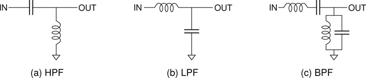
Figure 13.15 Simple LC high pass, low pass, and band pass filter circuits.
However, as illustrated in Figure 13.16, care must be taken in order to avoid excessive resonances and other response irregularities. The response variations shown are a result of different interfacing impedances of the circuitry to which the filter is connected. The under damped case, with a bit of resonance coming in at the cutoff frequency is a characteristic which is often actively encouraged in audio circuits, where ‘resonant filters’ can provide an excellent character to the tone of the circuit. Once again, the importance of well chosen interfacing impedances becomes clear, as the surrounding circuit plays a crucial role in the performance of the filter section.
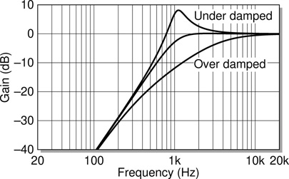
Figure 13.16 Simple LC high pass filter frequency response with resonance.
LC Resonance Frequency and Characteristic Impedance
As was previously seen in Figure 13.6, capacitor impedance falls with rising frequency and inductor impedance rises with rising frequency. As such there is always a single frequency at which the two components in any circuit consisting of a capacitor and an inductor will have the same impedance. This is represented in Figure 13.6 as the point at which the two lines on the graph cross. It thus follows naturally from Eq. 13.9 that for a capacitor and inductor in series there is a frequency at which the combined impedance of the circuit equals zero (when XC equals XL).
Similarly if the capacitor and inductor are instead placed in parallel then the impedance at this same frequency will instead rise towards infinity.a Figure 13.17 illustrates this behaviour, plotting impedance against frequency for circuits consisting of a capacitor and an inductor in series and in parallel respectively.
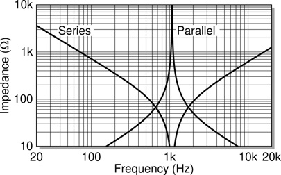
Figure 13.17 LC series and parallel impedance against frequency.
This frequency where the impedances become equal is called the resonant or natural frequency of the circuit, commonly indicated f0, and is readily calculated for any given capacitor-inductor pair by the equation shown in Eq. 13.15.
_________________________
It is a simple matter to derive this equation directly from the two impedance equations previously given in Eq. 13.1 and Eq. 13.2. Simply set the two expressions equal to each other and rearrange in order to make frequency the subject of the equation. The reader is encouraged to attempt this derivation as an exercise. This resonance property can be very useful and is widely used in, for instance, tuned circuits in radio receivers. It also represents the cutoff frequency which is achieved in an LC filter circuit.
A simple LC circuit also has a characteristic impedance, Z0, as defined by Eq. 13.16. This value can be important when designing LC circuits. As alluded to above, in order to control the resonance peak which can be exhibited by an LC filter and maintain a reasonably flat frequency response in the pass band the interfacing circuitry before and after the filter should have impedances close to this characteristic impedance. Alternatively a desired degree of resonance can be achieved by moving away from this optimum interfacing impedance in order to derive some interesting sonic effects when using these filters.
Without getting into a detailed derivation or analysis, it is instructive to note that multiplying the expressions for capacitive and inductive reactances (Eq. 13.1 and Eq. 13.2) yields L/C. This quantity has units of ohms squared and so applying a square root operation gives a quantity with units of ohms. While not a proof of the validity or meaning of the expression given for the characteristic impedance these observations do illustrate the relationship which the given equation bears to the reactances of the component parts of the circuits in question.
More often the design question to be answered is not ‘What f0 and Z0 correspond to given values of L and C?’ but rather the other way round. If a filter with a specific cutoff frequency and characteristic impedance is required, what values of L and C should be chosen? The mathematical rearrangement of Eq. 13.15 and Eq. 13.16 to find expressions for L and C is not complex. The interested reader is encouraged to work through the derivation for themselves. The resultant equations are shown below.
The shape of these equations should come as no surprise. This is the third time the same basic form has been encountered in this chapter, with terms rearranged as appropriate. The first instance is the capacitor and inductor reactance equations (Eq. 13.1 and Eq. 13.2) where the reactance (XC or XL) at frequency f is established. The second stems from the RC and RL filter cutoff frequency equations where in combination with resistor R they yield cutoff frequency fc, and the third instance, encountered here, has the characteristic impedance Z0 and resonant frequency f0 provide the ohms and hertz terms respectively.
Eq. 13.17 and Eq. 13.18 can be useful in the design of an LC filter, but possibly even easier to use and of even more utility is the kind of reactance chart shown in Figure 13.18. This kind of graphical lookup table, which equates to a pictorial representation of the two equations, is common in engineering references (e.g. Ballou, 2008a, p. 271), and proves a useful and easy to use design tool. Consider for example a design goal to reproduce the stepped LC high pass filter described in Williams (2012). Ten cutoff frequencies are listed for the ten steps of the high pass filter ranging from 70Hz to 7.5kHz.
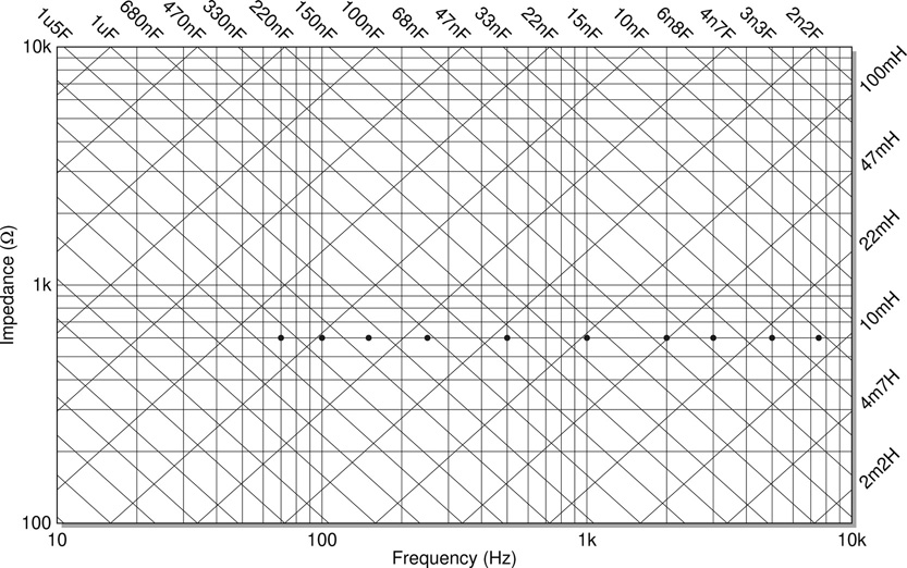
Figure 13.18 Reactance chart for the design of LC filters. The dots along the 600 line indicate the ten target frequencies in the example filter design task discussed in the text, simplifying the task of selecting suitable L and C values.
Clearly the switched filter sections will each interface with the same drive and load circuitry and as such all filters should share the same characteristic impedance in order to achieve consistent interfacing. Further research indicates that 600 is the most likely original characteristic impedance. Using the reactance chart it is a simple matter to take a horizontal line at the 600 level and identify points along this line for each of the desired cutoff frequencies, and thus appropriate LC pairs can be selected for each of the ten filters to be implemented.
It is important to also recognise that in the real world capacitors and especially inductors are only available in a limited set of values. By marking only the available values on the chart it is a simple matter to choose the best fit values for L and C. Furthermore if, for instance, the accuracy of the cutoff frequency is more important, while closely matched characteristic impedances are deemed to be less critical it is a simple matter to scan the chart visually to make the best possible design choices. Similarly, if extra resonance is to be preferred over excessive damping, again the chart allows a quick scan to yield the optimum values. Attempting the same procedure using Eq. 13.17 and Eq. 13.18 is much more cumbersome.
References
G. Ballou, editor. Handbook for Sound Engineers. Focal Press, 4th edition, 2008a.
G. Ballou. Resistors, capacitors, and inductors. In G. Ballou, editor, Handbook for Sound Engineers, ch. 10, pp. 241–272. Focal Press, 4th edition, 2008b.
P. Baxandall. Negative-feedback tone control. Wireless World, 58(10):402–405, 1952.
S. Niewiadomski. Filter Handbook – A Practical Design Guide. Newnes, 1989.
S. Niewiadomski. Sharper by design. Practical Wireless, 80(9):34–35, 2004.
D. Self. Small Signal Audio Design. Focal Press, 2nd edition, 2015.
B. Vogel. The Sound of Silence – Lowest-Noise RIAA Phono-Amps: Designer’s Guide. Springer, 2008.
A. Williams and F. Taylor. Electronic Filter Design Handbook. McGraw-Hill, 4th edition, 2006.
S. Williams. Tubby’s dub style: The live art of record production. In S. Firth and S. Zagorski-Thomas, editors, The Art of Record Production: An Introductory Reader for a New Academic Field, ch. 15, pp. 235–246. Routledge, 2012.