20 | Audio Transducers
Transducers come in a wide variety across many application areas. In the realm of audio electronics the two which come most readily to mind are microphones and loudspeakers. Others include coil pickups (standard electric guitar pickups) and piezo elements (which can operate as transducers in two directions – mechanical to electrical and vice versa). The standard spring reverb pan combines two transducers linked with springs. All these are examined in this chapter, along with some useful and interesting circuits using them.
Microphones
Microphones come in a range of types with vastly differing principles of operation. The two commonest classes in pro audio are the dynamic mic and the condenser mic. A particularly simple and inexpensive variant of the condenser mic is the electret condenser. Electret condenser mic capsules like those shown in Figure 20.1 are widely and cheaply available, and can be built into surprisingly effective condenser microphones relatively easily – probably the most significant difference between such circuits and good quality commercial microphones, which sets them apart, is actually the mechanical and acoustical design of the enclosure.
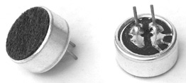
Figure 20.1 Electret condenser microphone capsules.
On top of the electronics considerations addressed here, much creative experimentation can go into the mounting and finishing of a project such as a microphone. For most electronics projects working on the enclosure can be every bit as fun and rewarding as the electronics, but it is primarily just a question of the aesthetics, and to some extent the general robustness of the finished project. On the other hand, most transducer circuits can have their performance significantly altered by the manner in which they are finished, with a well thought out and carefully constructed enclosure potentially making a great difference to the final success of the project. This can be particularly true of microphone projects. Inspiration in this regard can be found in sources such as Hopkin (1996), which, although focused on musical instrument design, provides lots of food for thought when it comes to acoustically active enclosures.
Phantom Powered Electret Condenser Microphone
With all this in mind, the phantom powered electret microphone circuit in Figure 20.2 makes a good starting point for the development of a homemade condenser mic suitable for use in recording interesting sounds with an individual character and a unique twist. As with all the major circuits throughout this book, possible breadboard and stripboard layouts are provided in Appendix D, but as always, have a go at your own layouts before resorting to the suggestions provided there. In this instance it might be useful to aim for a long thin stripboard layout so as to fit the finished circuit inside a slender enclosure, to make a good looking microphone.
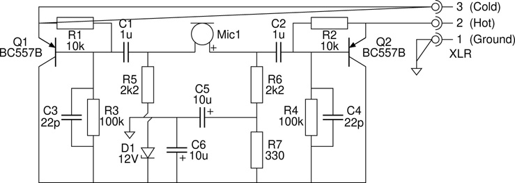
Figure 20.2 Phantom powered electret microphone circuit.
Figure 20.3 provides the necessary details for the transistor used in this circuit. Others can be substituted following the guidelines given in Chapter 17. As always, if an alternative transistor is to be employed, be sure to check the pinout for the particular part in question. Most crucially, notice here that the device used in this particular circuit is of the less common PNP type (with the arrow on the emitter pointing in, and the emitter itself operating at a positive potential relative to the collector).
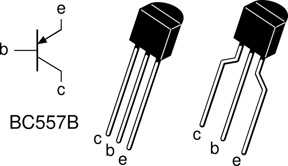
Figure 20.3 Pinout for the BC557B transistor used in the electret mic circuit given above. Note that this is a PNP device, and not the more commonly encountered NPN type. As usual it is always possible to try other transistors which look like they might be suitable replacements, but remember to confirm the specific pinout for any alternative device which you want to try.
Phantom powering is a commonly encountered method of providing power to an audio circuit such as a microphone or DI box. Notice in Figure 20.2 that no power supply connections are indicated, and the only external connections to the circuit are the three wires of a standard balanced audio connection (most typically implemented in the form of an XLR connector). In phantom powering the power is delivered to the circuit over the same wires across which the audio emerges (Figure 20.4). Pins two and three both present +48V delivered through 6k8Ω, with pin one supplying the common ground path necessary in order to complete the circuit and allow current to flow. A phantom power supply can only deliver a fairly modest amount of current into the circuit being powered (limited by the 6k8 resistors in the supply), so care must be taken in the design of such circuits.
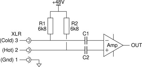
Figure 20.4 Standard phantom power supply configuration, as found in a phantom capable microphone input.
In drafting the schematic layout in Figure 20.2 the clarity of the circuit was better served by a neater layout, at the expense of the ‘positive at the top, negative at the bottom’ schematic diagram convention. Thus the ground connection, representing the most negative point in this circuit, is located in the middle of the diagram. This point attaches to pin one of the XLR.
The common connection point running along the bottom of the diagram is connected to this ground point through a 12V Zener diode (D1). This holds the collectors on the transistors, and all the other components connected here, at a potential of approximately +12V. The two emitters see the phantom power supply directly through the 6k8 resistors at the far end of the XLR. They are held at 48V minus whatever is dropped across these resistors. The microphone capsule itself drives the two bases through C1 and C2, providing the two anti-phase signals which ultimately drive the hot and cold outputs.
Loudspeaker Drivers
Just as the microphone is commonly found at the start of the audio electronics signal pipeline, so the loudspeaker often represents the end of that chain. Loudspeakers come in a variety of types, but by far the most frequently encountered is the moving coil loudspeaker (Figure 20.5). This consists of a coil of wire suspended in a magnetic field and attached to the loudspeaker’s cone. An AC signal in the coil generates a varying electromagnetic force, which causes the coil, and the attached cone, to move, producing sound.
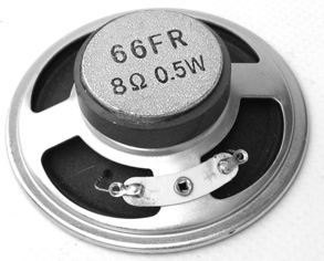
Figure 20.5 A typical low power moving coil loudspeaker driver.
A moving coil loudspeaker has two terminals usually labelled plus and minus. These terminals connect to the ends of the coil within the device. There is no functional difference between the two terminals and often it makes no difference in which order they are connected to a signal source. The only time when the order becomes important is when two or more drivers are being used in conjunction. In this case it is important that all drivers use the same wiring convention, otherwise drivers will be operating in opposite polarities, one pushing as the other one pulls and vice versa. This can lead to acoustic cancellation, resulting in very ‘thin’ sounding audio. In its commonest wiring configuration a speaker’s minus terminal is wired to the common circuit ground, while the plus terminal is driven by the amplifier signal, as in Figure 20.6.
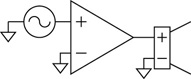
Figure 20.6 Basic loudspeaker wiring.
The two most basic specifications for any moving coil loudspeaker are its characteristic impedance and its power handling capability. By far the commonest impedance encountered is 8Ω, with 4Ω and 16Ω also being common. Most amplifiers will specify the minimum impedance load which should be attached to their output – four ohms is common but other limiting values are encountered also. Attaching a load with an impedance lower than the specified minimum will result in excessive distortion and may even cause damage to the amplifier.
The power handling capability of a loudspeaker is measured in watts. Exceeding this limit likewise incurs increased distortion and runs the risk of blowing the speaker, most commonly by overheating the voice-coil to the point where the wire burns through. The speaker shown in Figure 20.5 is a small (two and a half inch diameter), low power unit. As can be seen in the image it has an impedance of 8Ω, and is rated to handle just half a watt (0.5W). A small speaker like this works well with the 386 based amps presented here and elsewhere.
Coupling Capacitor
Often a capacitor will be placed between the amplifier output and the loudspeaker in a circuit design. The fundamental requirement which such a capacitor is intended to meet is that there be no DC component to the signal present across the loudspeaker’s terminals. This is important for two reasons. Firstly, a DC component will result in the loudspeaker cone adopting an offset resting position, resulting in elevated distortion in the audio it produces. Secondly, a DC voltage will result in a corresponding DC current constantly flowing through the loudspeaker coil. This will result in an excessive heating effect, especially when no AC signal is present to keeping the coil moving back and forth, cooling it down. The inevitable result is a burned out speaker coil.
This observation leads to a perhaps unexpected conclusion for the matching of amplifiers and loudspeakers. It is obvious that a low power handling speaker should not be connected to a more powerful amplifier, as the amp is likely to blow the speaker when turned up. It may not be so obvious that the opposite arrangement – low power amp and high power speaker – also has the potential to blow the speaker. The amp, being lower power, is more likely to be overdriven and start clipping badly. Clipping sends repeated short bursts of high current through the loudspeaker coil, without any heat dissipating movement accompanying it, and so burnout can once again ensue.
When considering whether or not an output capacitor is required between amp and speaker, the quiescent voltage level at the output of the amp needs to be compared to the voltage level at the other speaker terminal. If they are the same, no capacitor is needed. Consider the two circuit configurations illustrated in Figure 20.7. In each case the minus terminal of the loudspeaker is connected to ground. Thus, when no signal is present at the input of the amplifier, the plus terminal of the loudspeaker must also sit at ground potential.
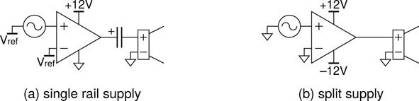
Figure 20.7 The role of an output coupling capacitor.
An audio amplifier needs to be able to amplify the positive and negative portions of an audio signal equally well. It can only produce outputs in the range of voltages available from its power supply, and therefore with no input signal the output must sit at a voltage half way between its positive and negative power rails. In Figure 20.7a a single rail supply is utilised. The midpoint in this case is +6V, and so this is where the output will sit. With the minus terminal of the speaker connected to ground (0V), clearly a DC blocking capacitor is needed between the amp and the plus terminal of the speaker. On the other hand, in Figure 20.7b a split supply is shown powering the amp. With its power rails at +12V and −12V, its output will sit at 0V, thus matching the ground potential on the minus speaker terminal, and so no capacitor is required.
Notice that the capacitor indicated in Figure 20.7a is shown as a polar type. The capacitor will act as a high pass filter, and since it is attached to a relatively low impedance in the form of the loudspeaker, it needs to be quite large in order not to block too much low frequency content from the audio signal. Large capacitors are most often polar, which is why this device is marked as such. The cutoff frequency of this high pass filter can be calculated using Eq. 13.13. A smaller value can be used to restrict lower frequencies, which might be desired when driving a small, low power handling driver such as the little half watt unit illustrated in Figure 20.5.
Bridge Mode Connection
There are two situations in particular in which the coupling capacitors discussed above are not needed: split rail and bridge mode operation. The split rail case has been addressed. Figure 20.8 illustrates the second situation, that of a bridge mode amplifier configuration. The requirement, as previously stated, is that no DC component exists across the terminals of the loudspeaker. The bridge mode configuration is unusual in that the minus terminal of the loudspeaker is not connected to ground. Instead the speaker floats around the quiescent output level of the amplifiers attached to the two terminals. Clearly these two amps must have matched outputs, so as to maintain the required equal quiescent levels, and avoid any unwanted DC current flow.
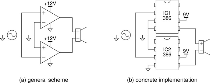
Figure 20.8a illustrates the basic bridge mode configuration: two differential amplifiers with the same signal fed to the noninverting input of one and the inverting input of the other. The other inputs are grounded, and the speaker is bridged across the two outputs (hence the name). In this case the amplifier powering scheme can be single or split rail, without the need for coupling capacitors in either case.
Figure 20.8b shows a simple concrete implementation of the bridge mode configuration using a pair of 386 low power audio amplifier ICs. Pins two and three are the inputs. The input signal is fed into pin two on IC1 and pin three on IC2, with the other input pins grounded. Pin five is the output on each chip, connected here to either terminal of the loudspeaker.
With absolutely no other components required apart from input, output, and power, this must be a contender for the simplest amp ever (alongside the bare-bones amp in Figure 18.8a, which uses just one 386, but does require an output capacitor in addition). In this very simple circuit pins one, seven, and eight are left unconnected. Obviously there are many enhancements which could be applied to this basic design, but it does operate quite effectively even as shown.
One further point must be given careful attention when examining a bridge mode configuration, that of amplifier loading. As previously stated, an amplifier will have a minimum load impedance, perhaps 4Ω. In the bridged configuration it is important to note that each of the two amplifiers involved sees only half of the load connected between them. Recall that load impedance is measured to ground, and note that there is a virtual earth point half way along the speaker’s voice coil, with the terminal voltages seesawing up and down either side of it. Therefore, the speaker (or combination of speakers) connected across the amplifier outputs must have an impedance of at least twice the amplifiers’ minimum load impedance.
Stabilisation Network
One other circuit element which is very often seen in conjunction with a standard moving coil loudspeaker is shown in Figure 20.9. This is what is usually referred to as a zobel network. In simple circuits, the network usually takes the form of a small resistor (usually 10Ω) and a capacitor (often around 47nF) in series. A lot of work and a lot of maths can go into modelling and designing ideal solutions, but the simple approach serves well for all but the most demanding applications.
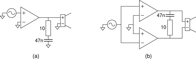
Figure 20.9 Stabilising a loudspeaker with a zobel network.
Electrically, a moving coil loudspeaker can be thought of as a resistor and an inductor in series. It is made from a coil of wire, so this should come as no surprise. Inductors have a frequency dependant impedance (Eq. 13.2). As such, if an amplifier has just a loudspeaker attached to its output, it will see a load which varies widely with frequency. A zobel network has an impedance which varies in the opposite direction – the speaker has inductance while the zobel network has capacitance.
The commonest moving coil loudspeakers have a quotes resistance of 8Ω, so the 10Ω resistor in the network matches this closely enough. The net result of the speaker and zobel in parallel is a load with a much more consistent impedance across the operating frequency range of the amplifier. This steadier loading tend to make an amplifier behave better.
Wiring Drivers in Series and Parallel
As mentioned above, loudspeakers have as one of their primary figures of merit, a characteristic impedance, the commonest being 8Ω, and likewise amplifiers have a minimum load impedance. It is a common situation to find multiple loudspeaker drivers wired together and connected to a single amplifier output (think of a guitar amp driving a two or four speaker cab). In such a case it is important to know how to determine the total impedance which a particular speaker combination will represent.
In actual fact it is very straightforward in most cases. The familiar resistor series and parallel rules are all that is required. Indeed, for almost all wiring configurations likely to be encountered the situation is even easier. It is usually the case (and usually the only advisable course) that only identical drivers are wired in combination like this (LF/HF combinations involving a crossover are a different matter, and are not covered here.)
Revising the series and parallel rules from Chapter 12, it quickly become apparent that two equal resistances in series result in a total resistance double the size, while two equal resistances in parallel results in a total half the size. So for instance, two 8 drivers in series looks like 16Ω, and two 8Ω drivers in parallel looks like 4Ω, see Figure 20.10.
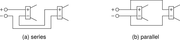
Figure 20.10 Wiring two loudspeakers in series (a) and in parallel (b). For loudspeakers of equal impedance ZLS, two drivers in series: Zseries = 2ZLS, and two drivers in parallel: Zparallel = ZLS/2.
Using a Speaker as a Dynamic Mic
The section on microphones earlier in this chapter focused on the commonly available electret condenser microphone capsule. Condenser microphones represent one of the two key microphone types found in audio work. The second type is the dynamic microphone. In many ways the dynamic mic is a more straightforward device than the condenser. Fundamentally it shares exactly the same working parts as the moving coil loudspeaker – in fact, so much so that it turns out to be a simple matter to use a moving coil loudspeaker as a microphone.
The key differences between the two are size and mass. Generally the detection element of a microphone (the diaphragm) is small and light so that sound can move it around easily. The equivalent part of a loudspeaker (the cone) tends to be much more bulky, so it can move a lot of air. So for a speaker to work effectively as a mic, it should be relatively light and the sound it is to be used to detect should be relatively energetic (i.e. loud and low frequency). Spend any time in a recording studio and you are bound to come across the NS-10 kick drum microphone or its commercialised variants. Basically its just a mid sized driver used as a microphone on loud, low frequency sources.
Coil Pickups
In common with dynamic microphones and moving coil loudspeakers, coil pickups operate on the principle of electromagnetic induction. In dynamic mics, a conductor moving in a magnetic field generates an electrical signal. In moving coil loudspeakers the process is reversed with an electrical signal in a conductor mounted in a magnetic field generating movement. Thus electromagnetic induction usually involves a conductor moving in proximity to a magnet.
Coil pickups represent something of a twist on this idea, in that the conductor and the magnet do not move relative to one another; both are firmly mounted in place within the pickup body, as illustrated in Figure 20.11. Instead a metal guitar string – which is not involved in the electrical circuit – vibrates in the magnetic field, causing a signal to be induced in the stationary coil of the pickup. As the metal string vibrates in the magnetic field, it deforms the field, effectively dragging it back and forth through the coil in the pickup, thus generating the requisite electrical signal. So rather than the conductor moving in the magnetic field, as is the more familiar incarnation of electromagnetic induction, the magnetic field actually moves through the conductor. The effect is however the same; a signal is induced in the conductor.
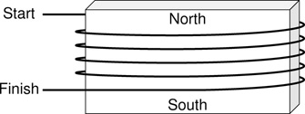
Figure 20.11 Structure of a standard single-coil electric guitar pickup.
Coil pickups come in two basic forms, single coil and humbucker pickups, as illustrated in Figure 20.12. The biggest problem with the basic single coil pickup is that a coil of wire can work like an ariel, detecting electromagnetic radiation floating through the air. Single coil pickups are known for being quite noisy in this regard. The solution is the humbucker. The ariel action of the pickup, mopping up stray noise, is independent of the magnet in the pickup, whereas the wanted signal induced by the vibrating string is directly dependent on the magnet. This difference can be used in order to retain the wanted signal while rejecting the unwanted airborne interference.
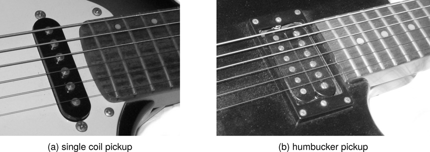
Figure 20.12 A single coil and a humbucker electric guitar pickup.
A standard single coil pickup can be manufactured in two basic configurations, sometimes referred to as ‘south to strings’ and ‘north to strings’, depending on the orientation in which the magnet has been inserted into the assembly. This distinction is illustrated in Figure 20.13. The methods of constructing a pickup vary from manufacturer to manufacturer, and from one pickup model to another, but often it is the case that pickups are constructed such that it is relatively easy to remove and rotate the magnet, in order to reconfigure the pickup if required. Manufacturers will usually provide guidance to the process if such a procedure is possible with their particular devices.
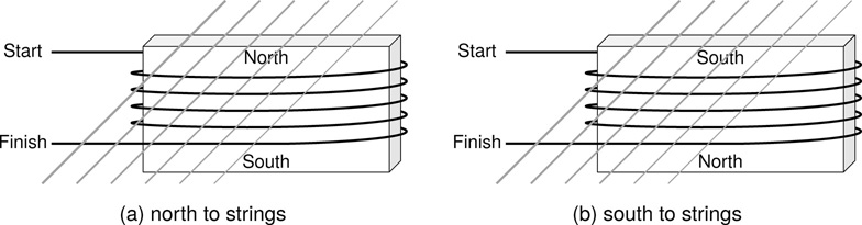
Figure 20.13 The magnet orientation can differ between different pickups.
Humbucker Pickups
To make a humbucker requires two single coil pickups whose magnets are mounted in opposite orientations. (In fact humbuckers often use a single magnet installed so as to direct its two poles one at each of the pickup windings.) The two pickups in a humbucker are placed side by side but are wired together out of phase, as in Figure 20.14. Each pickup generate both the wanted and unwanted signals described previously. The out-of-phase wiring means that the unwanted signal (which is not affected by the magnet orientations) cancels between the two pickups. The wanted signals however get flipped twice, once by the out-of-phase wiring and again by the reverse oriented magnets. This means that the wanted signals from the two pickups end up back in the same polarity and thus adds, actually giving a stronger signal.
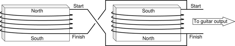
Figure 20.14 How to wire two single coil pickups in a humbucker configuration.
With two binary options (wiring phase and magnet orientation), there are four possible ways in which two single coil pickups can be wired together, and four corresponding types of behaviour. These four possible variations are laid out in Table 20.1. While many factors combine to make up the final tone emanating from an electric guitar, these basic wiring options can certainly prove a useful tool in tailoring the sound of an instrument.
Configuration |
In-phase |
Out-of-phase |
||
N-to-strings |
S-to-strings |
N-to-strings |
S-to-strings |
|
Signal |
|
|
|
|
Noise |
|
|
|
|
Result |
Both add |
Signal cancels, noise adds |
Both cancel |
Signal adds, noise cancels |
Comments |
Same as single coil |
Worst of both worlds |
Thin sound, can be useful |
Standard humbucker |


Other considerations not discussed here include: series versus parallel pickup wiring, choice of magnet type (there are several), pickup positioning along the guitar body, and proximity of pickup to strings. Some pickups even have per-string magnet pole-pieces which can be individually adjusted to modify their response. And then there are many non pickup related factors, from the strings, to the guitar body, to the amp, all of which play a role – interesting topics but not for the current discussion.
To round off this section on coil pickups, a simple electric guitar wiring diagram is presented (Figure 20.15). The two pickups indicated may be single coil variants, or they may represent complete humbucker pickups, or indeed other nonstandard wiring pickup pairs. If single pickups are assumed then it is certainly worth checking the magnet orientation of the pair. If they are opposite (or if one can easily be converted, as discussed above), then it might be advantageous to wire them out of phase to form a humbucker pair, even if they are not mounted right beside each other. The dot at the top of each coil indicates that these two are wired in phase. Swapping the two connections to one of the coils is all that is needed to place the two coils out of phase.

Figure 20.15 Typical wiring diagram for a basic two pickup electric guitar.
Pickup selection switches can be far more elaborate than the one shown here. In this case the three switch positions simply select one, the other, or both pickups in parallel. The symbol indicates an dpdt on-on-on device, and ‘NC’ stands for ‘no connection’. A standard dp3t switch could also be used here, with jumper wires between the appropriate two pairs of throws.
The tone stack is a fairly standard arrangement for an electric guitar. With the pot turned up, the large resistance means little signal goes down that way, and the signal from the pickups passes un-affected. As the pot is turned down, the capacitor continues to block low frequencies from shunting to ground, but high frequencies can make their way through. Thus the tone control works by bleeding off more or less of the high frequencies from the incoming signal, depending on the position of the pot control.
Finally, the volume pot is absolutely standard, simply tapping off its output signal somewhere between full and zero, depending on the position of the pot knob, and the guitar output is provided via a standard TS jack.
Piezo Elements
Piezoelectric material has a very simple, very useful two way behaviour. If it is deformed (for instance bent) an electric charge appears on its surface, with opposite charges appearing on opposite faces. If the direction in which it is being bent is reversed, then so too does the sign of the charge on each face. Alternatively, if a charge is applied to its faces, then as a result it physically bends. Again, reversing the polarity of the charging signal reverses the direction of the bending which results.
Thus a vibration which is allowed to deform some piezoelectric material will produce an equivalent electrical signal between its two faces, and correspondingly, if an alternating signal, such as an audio signal, is connected across the faces of the material, then it will vibrate with the signal.
Thus piezo elements can be used as pickups or contact microphones, and they can be used as drivers or sounders. The piezoelectric material itself is a hard, brittle crystalline substance. In the piezo elements most commonly encountered, the material itself is adhered to a solid brass disc, in order to give it strength, and to provide a good electrical contact right across its back face.
The exposed top surface is covered in a slivered coating to form a second electrical contact, and typically two wires are soldered on, one to the brass disc and one to the silvered front surface, as shown in Figure 20.16a. Sometimes alternative electrical connection methods might be found. For instance, the buzz tester in most multimeters is implemented using a piezo element, and it is likely that the connections in such a device are made using carefully placed springs which contact the piezo disc when the multimeter case is put together. This technique avoids the need for soldering (which can be tricky with piezo discs, and easily broken).
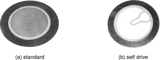
Figure 20.16 Two piezoelectric elements. A standard two terminal device and a self drive variant with a third ‘sense’ terminal.
As pickups, piezos are extremely easy to use; attach one to any amp input and you have a basic contact mic. Getting good quality sound out of them takes a little more effort. A piezo element presents an extremely high impedance, and so in order to maintain signal quality it is best to connect a piezo pickup to as high an input impedance as possible. Most typical audio inputs have input impedances no higher than a few tens of kΩs. Common guitar amps extend this up into the hundreds of kΩs range, which can be pretty good for a piezo, but even higher can be better. JFET buffers are commonly employed with piezos in order to get the most out of them. These are usually designed with an input impedance of one or two MΩs. The circuit in Learning by Doing 17.5 (p. 308) would be a good option for this application.
Piezos will not pickup sound travelling in the air; there just isn’t enough energy in an acoustic signal to bend the brass disc and generate a signal. The piezo element must be attached firmly to a vibrating surface in order to achieve good sound pickup. Figure 20.17 illustrates the kind of device which can be found. The piezo element is enclosed in the plastic housing, with a tough rubber pad providing good mechanical linkage, and a sprung clamp for attaching the pickup to a surface. This one is most likely to be found clipped to the sound hole of an acoustic guitar.
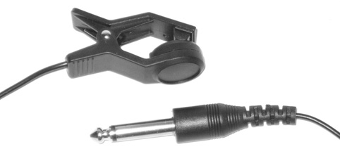
Figure 20.17 A piezo pickup with a spring clamp and a TS jack plug output.
Self Drive Piezo Elements
Figure 20.16b shown a less commonly encountered variant on the basic piezo element. In this type the top silvered contact area is separated into two unconnected zones – the main drive contact, and a smaller feedback region used to sense when the element has been deformed. These three terminal types are called self drive piezos, and are most commonly used to implement very simple oscillator sounders, as examined next in Learning by Doing 20.6. Regular piezos can also be used to reproduce a full audio signal (typically at a low fairly quality). Refer back to Learning by Doing 14.2 (p. 255) for an example of how to drive a piezo sounder with an audio signal.
Reverb Pans
A spring reverb pan (Figure 20.18) is not strictly speaking a transducer; it takes as its input an electrical signal and produces as its output another electrical signal. However internally it actually consists of two transducer elements linked by one or more springs. The first transducer converts the incoming electrical signal into mechanical movement, which sends vibrations along the attached springs. These vibrations reflect back and forth along the springs producing the desired reverb effect. The movements within the springs also couple into the second transducer which is linked into the far end of the springs. This transducer operates in the reverse direction converting the spring’s vibrations back into an electrical signal which appears at the output connection of the pan.
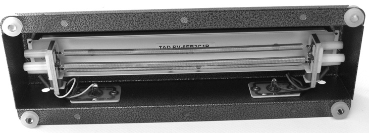
Figure 20.18 A TAD (Tube Amp Doctor) 8EB2C1B reverb pan.
References
J. Borwick, editor. Loudspeaker and Headphone Handbook. Focal Press, 3rd edition, 2001.
N. Collins. Handmade Electronic Music. Routledge, 2nd edition, 2009.
R. Fliegler. The Complete Guide to Guitar and Amp Maintenance. Hal Leonard, 1998.
B. Hopkin. Musical Instrument Design. See Sharp Press, 1996.
W. Leach. Impedance compenstion networks for the lossy voice-coil inductance of loudspeaker drivers. Journal of the Audio Engineering Society, 52(4):358–365, 2004.