9 | Basic Circuit Analysis
Before moving on to examine electronic components and how to use them it is worth taking some time to bring together key details of the most important primary electrical quantities which have been encountered so far, and to introduce four very simple but very important laws which facilitate a great deal of circuit analysis, providing the tools for many useful calculations to be performed on the circuits and systems which are encountered throughout the rest of this book. A good understanding of these quantities and these laws will help to develop an appreciation of what can be expected to happen in any given circuit and why things work the way they do in electronic circuits and systems.
Many other rules and equations, specific to particular components or particular circuit configurations are introduced at appropriate points throughout the rest of the text. These are gathered in Appendix B – Quantities and Equations. Together they provide the tools to analyse and design many useful circuits, and form the basis for a deeper understanding of the topics presented. As stated from the outset, this book aims first and foremost to provide an accessible introduction to audio electronics, avoiding too much in depth mathematical analysis. That being said, a firm grasp of these relationships can only be a good thing in assisting the reader to get the most out of their endeavours in practical audio electronics. While much of the maths can be skimmed on a first reading, returning to it and developing that deeper understanding is to be highly recommended.
Primary Quantities
Table 9.1 provides a reminder of the four most important fundamental quantities which have already been encountered: ohms, volts, amps, and watts. A firm grasp of what these concepts relate to and how they interact with each other makes all subsequent circuit analysis much easier to grasp.
Quantity |
Units |
Notes |
||
Impedance |
(Z) |
Ohm |
(Ω) |
also Resistance (R) and Reactance (X) |
Voltage |
(V) |
Volt |
(V) |
aka EMF, PD |
Current |
(I) |
Amp |
(A) |
aka Ampere |
Power |
(P) |
Watt |
(W) |
also Apparent Power (VA) |
Impedance is a vector quantity made up of two components, resistance and reactance. In this context a vector can be thought of as simply a quantity that has both magnitude and direction. For the purposes of this book only the magnitude (i.e. size, measured in ohms) is needed. The direction, or phase (measured in degrees) becomes important when more advanced and detailed analyses are being performed. Those familiar with audio theory will recognise phase as an important feature of how sounds interact with one another. No deeper understanding of the concept is needed here.
Impedance is a property which electronic components exhibit, representing their opposition to the flow of electricity. For some devices (e.g. resistors) it is a simple, constant value, while for others its magnitude and its behaviour depend on the circuit conditions at any given time. This more dynamic aspect of impedance is revisited when capacitors are introduced in Chapter 13.
Voltage is the electrical pressure or push which attempts to make electricity flow. A number of other terms can be used to refer to the same phenomenon. Electromotive force (EMF), potential difference (PD), and electrical tension all mean basically the same thing as voltage, although each is typically encountered in its own specific context.
Current is measured in amperes (often shortened to amps). The terms amperage or ampage are sometimes encountered, usually referring to the amount of current a particular device can be expected to draw under normal conditions or the amount of current which a device can handle before failing (e.g. What is the ampage of the fuse in that plug?).
Power in watts is used to measure the rate of energy usage in a circuit. The term wattage is sometimes used to refer to the amount of power a device can be expected to use (e.g. What’s the wattage of that light bulb?). Apparent power, which has units of volt-amps (VA) rather than watts, includes both the power which is used up in a circuit and also the power which goes into but later comes back out of a circuit. This second element is called reactive power. Components like capacitors and inductors can store and later release energy, and as such can introduce an element of reactive power to the power usage of devices which involve them. Apparent power is worth being aware of but is of no real consequence in the context of this book.
Ohm’s Law
Ohm’s law states a very simple relationship between voltage, current, and resistance. It can be used to calculate the behaviour of very many circuits and is probably the single most useful calculation to know when it comes to working out what is going on in pretty much any electrical system. Some care needs to be taken when applying it to circuits which involve components other than simple resistances. This is addressed in more detail as these components are encountered along the way. The basic relationship represented by Ohm’s law, as shown in Eq. 9.1, forms the bedrock of a solid understanding of electricity and electronics.
|
(9.1) |

The triangle figure accompanying the equation is a useful way to remember how the law is used in different situations. As with any mathematical equation of this very simple form (A = B × C) it can be used in three different variations depending on which two things are known and which one is required to be calculated. If current and resistance are known and voltage is to be calculated it is a simple matter of using the equation as presented. If however the quantities which are known are voltage and resistance, and it is the current which is to be calculated then multiplying the two known values does not result in the correct answer. In fact one needs to be divided by the other. In order to see which should be divided by which, the triangle can be used. In this case the required new equation can be read off from the triangle figure as I = V/R. Similarly if R is the unknown then R = V/I can be arrived at from inspection of the triangle figure with equal ease. Thus the triangle figure allows the user to extract any of the three variations on Ohm’s law with ease and in confidence that the correct relationship has been used.
Watt’s Law
Watt’s law, as shown in Eq. 9.2 provides for the calculation of power. Often different components can cope with different amounts of power, and so it can be important to calculate the power which will be dissipated in a circuit or in a particular component. In this way it is possible to ensure that components will not overheat and be damaged or destroyed if used in a particular circuit.
|
(9.2) |

The description presented above for the use of the triangle figure in Ohm’s law holds equally well for Watt’s law, which follows the same basic A = B × C pattern. It should therefore be obvious that the two variations not explicitly shown in Eq. 9.2 above are I = P/V and V = P/I. Again, given any two of the three quantities the third can always be calculated.
Kirchhoff’s Current Law (KCL)
Kirchhoff’s current law, often abbreviated to KCL, states that the sum of the currents into any point in a circuit must equal the sum of the currents out of the point. What this most commonly means in practice is that if a branch point is encountered in a circuit, where three or more components meet (a very common configuration), and the currents flowing in all but one of the branches are known or have been calculated then the current in the final branch is known by extension.
If the common image of water flowing in pipes is used to illustrate electrical current then Kirchhoff’s current law becomes quite apparent. Whatever water flows into a junction in a network of pipes has to flow back out, there is nowhere else for it to go, and likewise no more water than that which has flowed in can flow out.
Kirchhoff’s Voltage Law (KVL)
Kirchhoff’s voltage law (KVL) states that the sum of all the voltage drops around any loop or closed path in an electric circuit is zero. In other words starting at any point in a circuit, moving from point to point along any path, and finishing up back at that same initial starting point, measuring the voltage changes as each new point is visited and adding them all up results in a final answer of zero volts. Imagine starting at any point on the side of a mountain and moving up and down to any number of other points, higher and lower on the side of that mountain, and finally arriving back at the starting point. The starting altitude is equivalent to the initial voltage. Each subsequent altitude corresponds to a new voltage. In order to arrive back at the same point, any movement up the hill must eventually be balanced out by an equal amount of movement down the hill, and vice versa, and so when arriving back at the starting point the sum of all the altitude changes equals zero.
When using Kirchhoff’s voltage law the path taken around the circuit may or may not take in any power sources such as batteries which are present in the circuit, the law works for any path. Usually the loop of interest in any analysis is quite compact, but in theory the path considered can be as long and convoluted as required. The direction of travel around the loop is also irrelevant, all positive voltage steps simply become negative and likewise all negative voltage steps become positive, thus resulting in the same zero sum around the loop.
Kirchhoff’s two laws are explicit statements of two underlying principles of electricity. More often than not they will be applied intuitively during a circuit analysis without ever making direct reference to the formal statement of the basic principles. Unlike Ohm’s and Watt’s laws, they tend not to be used for performing specific calculations, but rather help to guide the overall understanding of what particular circuit conditions will arise in any given situation. It is somewhat more common for them to be referenced (usually using the shorthand KCL and KVL) in a written description accompanying or replacing a more mathematical treatment of a problem.
Applying the Four Laws
The initial presentation of the four laws given above was kept deliberately brief, without examples or significant explanation. A few simple applications and instructive examples are presented here in order to clarify the use of the laws and to explore their implications.
Example One – Battery and Bulb
Consider the circuit shown in Figure 9.1. The battery is labelled as providing 1.5V. On its own this does not provide enough information to work anything else out. However if it is also given for example that the bulb has a working resistance of 15 it is now possible to calculate a) the amount of current which will flow in the circuit and b) the amount of power which it will dissipate.
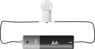
Figure 9.1 Battery and bulb diagram using nonstandard informal pictographic notation.
The first question to ask when addressing any problem of this kind is ‘What is known and what is needed?’. In this case voltage and resistance are known, and current and power are needed. This leads to the question ‘Is there a rule or law which involves only the known quantities and one of the unknowns?’ In this case there are two possible routes which could be followed. Ohm’s law (V = I × R) fits, with current as the one unknown, and so does the second variant of Watt’s law (P = V2/R), with power as the one unknown. It makes sense to answer the first part of the question first.
In order to calculate the current, Ohm’s law can be used. As stated above, the voltage provided by the battery, and the resistance of the bulb are known. This is a very simple circuit, with the bulb connected directly across the ends of the battery and no other components involved. As such Kirchhoff’s voltage law can be applied to see that the full voltage of the battery must appear across the terminals of the bulb. (See the next example for a case where the available voltage gets broken up between different components.)
To see how KVL is applied here consider starting at the minus terminal of the battery and moving around the circuit in a clockwise direction. There is only one possible loop in this very simple circuit. First the battery itself is crossed. This results in a positive voltage step of 1.5V, the difference between the negative and positive terminals of the battery. Continuing around the circuit the next thing which is encountered is the left hand terminal of the bulb. Crossing over the bulb and continuing on leads straight back to the starting point with no further circuit elements encountered.
KVL tells that the sum of the voltage drops around this circuit must be zero. The voltage drops encountered around the loop were: +1.5V crossing the battery and an unknown voltage across the bulb. For a zero sum this unknown voltage drop must therefore be −1.5V.
Note that traversing the loop in the other direction will lead to the same results with the signs reversed. This just indicates the fact that the left hand terminal of the bulb is at a potential 1.5V above the right hand terminal, and likewise the right hand terminal is at a potential 1.5V below the left (and likewise for the battery). This is a trivially simple application of KVL but it does provide a straightforward example of how it works.
Using Ohm’s law –
Following this calculation the new situation can be summarised as, voltage, current, and resistance are known, and power is needed. The only law involving power is Watt’s law, so this must be the one to use here. Since so many things are now known any of the three variants could be used (as was noted previously, variant two could have been used from the outset). Since it is available, it makes sense to use the primary form.
Using Watt’s law –
It is always worth doing a quick check where possible to make sure everything has been worked out correctly and no errors have crept into the calculation. In this case an obvious check would be to also calculate the power using Watt’s law variant two as previously mentioned. A calculator could be used but, observing that 1.5 = 0.1 × 15, the calculation is easy enough by hand:
150mW as was calculated above.
The pictographic representation of a circuit as used in Figure 9.1 is not a standard nor a very useful method for drawing circuits. More usually circuit diagrams are constructed using a set of standardised circuit symbols to represent the components involved. A detailed description of this scheme and its interpretation is given in Chapter 7, and a comprehensive list of commonly encountered symbols is provided in Appendix C. The simple, symbol based schematic diagrams in the rest of this chapter should be easy enough to interpret without further explanation. First off a standardised version of the circuit examined above is presented in Figure 9.2. This represents exactly the same circuit as was shown in Figure 9.1 above (with the additional information on the bulb’s working resistance added).

Figure 9.2 Battery and bulb schematic diagram.
Example Two – Resistors in Series
Figure 9.3 shows two resistors in series. The value of the first resistor is given, as is the current flowing through it, and the voltages at either end of the network are also provided. a) Calculate the value of the second resistor. b) Calculate the voltage at the point between the two resistors.
Note that in this case no complete circuit is actually shown. It is assumed that the circuit continues on from where the two voltages are specified eventually linking one side round to the other. This unknown section may be large or small, complex or simple, it makes no difference to the analysis of the shown section under investigation here.

Figure 9.3 Resistors in series.
Consider a point in the circuit between the two resistors. By KCL current in equals current out. Therefore the current flowing through resistor R must be 20mA, since this is what is entering the point coming from the 100Ω resistor and there is only one route out, through resistor R. The voltage from end to end is 12 − 2 = 10V, and the current from end to end is 0.02A, and so Ohm’s law can be used to determine the resistance from end to end. Since resistors in series simply add their values (see Chapter 12), it is clear that the value of R can then be determined.
Using Ohm’s law and the resistor series rule –
So the resistance of resistor R is 400Ω. Answering the second half of the question, what is the voltage between the two resistors, is now a simple matter based on all the information to hand. Applying Ohm’s law once again gets most of the way there, but there is a trap to be avoided. Ohm’s law will yield the voltage drop across either resistor, but this is not the same thing as the voltage at the midpoint.
When doing calculations always take great care in applying any multipliers which are present. In this case remember that milli- means divided by a thousand, and so in the above example 20mA becomes 0.02A. See Appendix A for details on all multipliers likely to be encountered.
Applying Ohm’s law to the first resistor –
However this 2V is not the voltage at the midpoint, it is the voltage difference between the two ends of the resistor. The other end of the resistor is at a voltage of 12V, and so the voltage at the midpoint is 12 − 2 = 10V.
To double check, the same calculation performed for the other resistor should lead to the same centre voltage since one point in a circuit can not be at two different voltages simultaneously.
Applying Ohm’s law to the second resistor –
This means that there are eight volts across the second resistor. The far end of the second resistor is at 2V. Eight plus two equals ten, so again the midpoint voltage comes out as 10V. Note that in the first case the voltage drop (2V) was subtracted from 12V while in the second case the voltage drop (8V) was added to 2V.
The voltage at the midpoint must be between twelve and two, and so in order to find it the appropriate calculations are either to subtract from twelve (coming down from the upper limit) or to add to two (going up from the lower limit).
As further verification of the answer, eight volts across one resistor and two volts across the other yields ten volts from end to end. There is a potential of twelve volts at one end and two volts at the other, so the difference between the two ends is indeed ten volts. It looks like the calculation is correct.
References
K. Brindley. Starting Electronics. Newnes, 4th edition, 2011.
A. Hackmann. Electronics: Concepts, Labs, and Projects. Hal Leonard, 2014.
P. Horowitz and W. Hill. The Art of Electronics. Cambridge University Press, 3rd edition, 2015.
P. Scherz and S. Monk. Practical Electronics for Inventors. McGraw-Hill, 3rd edition, 2013.
A. Sedra and K. Smith. Microelectronic Circuits. Oxford University Press, 7th edition, 2014.