CHAPTER 17

Adding Material Details with Maps

In addition to using materials, another way to enhance an object is to use a map—but not a roadmap. In Max, maps are bitmaps, with patterns that can be applied to the surface of an object. Some maps wrap an image onto objects, but others, such as displacement and bump maps, modify the surface based on the map's intensity. For example, you can use a diffuse map to add a label to a soup can, or a bump map to add some texture to the surface of an orange.

Several external tools can be very helpful when you create texture maps. These tools include an image-editing package such as Photoshop, a digital camera, and a scanner. With these tools, you can create and capture bitmap images that can be applied as materials to the surface of the object.

Understanding Maps

To understand a material map, think of this example. Cut the label off of a soup can, scan it into the computer, and save the image as a bitmap. You can then create a cylinder with roughly the same dimensions as the can, load the scanned label image as a material map, and apply it to the cylinder object to simulate the original soup can.

Different map types

Different types of maps exist. Some maps wrap images about objects, while others define areas to be modified by comparing the intensity of the pixels in the map. An example of this is a bump map. A standard bump map would be a grayscale image—when mapped onto an object, lighter-colored sections would be raised to a maximum of pure white; darker sections would be those regions where a minimal bump or no bump is applied. This enables you to easily create surface textures, such as the rivets on the side of machine, without having to model them.

Still other uses for maps include background images called environment maps and projection maps that are used with lights.

Maps that are used to create materials are all applied using the Material Editor. The Material/Map Browser provides access to all the available maps. These maps have many common features.

Enabling the global viewport rendering setting

To see applied maps in the viewports, select the Show Standard Map in Viewport button in the Material Editor or enable all scene maps with the Views Show Materials in Viewport As Shaded Display with Maps menu command.

For more accurate maps that show highlights, you can enable the Views Show Materials in Viewport As Hardware Display with Maps option. This is especially helpful when the scene objects use the Arch & Design materials. Hardware rendering in the viewport is available only when the Direct3D display driver is being used and if you are using a video card that supports hardware rendering.

Using Real-World maps

When maps are applied to scene objects, they are applied based on the object's UV coordinates, which control the size of the applied map. But, each bitmap can be sized along each axis to stretch the map over the surface. Another way to stretch a texture map is to resize the geometric object that the map is applied to. This is the default behavior of maps, but another option is available.

When a geometric object is created, you can enable the Real-World Map Size, which is generally next to the Generate Mapping Coords option. This option is also available when the UVW Mapping modifier is applied to an object. When enabled, this option lets you specify the size of the applied texture using scene units. When this option is enabled, it causes the texture maps to maintain their sizes as geometry objects are resized. Set the dimensions of applied texture maps in the Coordinates rollout.

Working with Maps

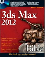
Maps are typically used along with materials. You can open most material maps from the Material/Map Browser. To open the Material/Map Browser if it isn't visible in the Slate Material Editor, select the Tools Material/Map Browser menu or press the O key in the Slate Material Editor. You also can open the Material/Map Browser by clicking any of the map buttons found throughout the Parameter Editor panel, including those found in the Maps rollout. Figure 17.1 shows this browser with its available maps.

In the Material/Map Browser all available maps are displayed by default in the Maps/Standard rollout, but if you have the Quicksilver Hardware or the mental ray renderer enabled, rollouts for mental ray maps and MetaSL maps are also displayed. If you right-click within the Material/Map Browser away from any rollouts and choose the Show Incompatible option from the pop-up menu, all map rollouts including mental ray maps are displayed even if the mental ray renderer isn't enabled.

FIGURE 17.1 Use the Material/Map Browser to list all the maps available for assigning to materials.

To load a map node into the Node View panel of the Slate Material Editor, simply double-click on it or drag the material from the Material/Map Browser to the Node View panel. All map nodes are easily identified by their green title bars in the Node View and Navigator panels.

Connecting maps to materials

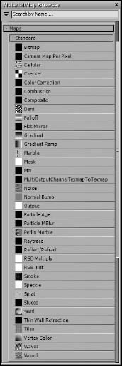
A map by itself in the Node View panel cannot be applied to objects in the scene. To add a map to a material it must be connected to one of the material properties. This is done by dragging on the map node's output socket and dropping the connecting line on the input socket for the material property where the map is being applied. For example, Figure 17.2 shows a connection between the Checker map node and the Standard material node's Diffuse Color. Once a connection is made, the material preview is updated to show that the applied map and the sockets at either end of the connection are highlighted green.

FIGURE 17.2 Map nodes need to be connected to material properties in order to show up in the material.

Double-clicking the map node's title opens the map's parameters in the Parameter Editor. Maps also can be applied by clicking on a map button in the Parameter Editor and selecting a map type from the Material/Map Browser that opens.

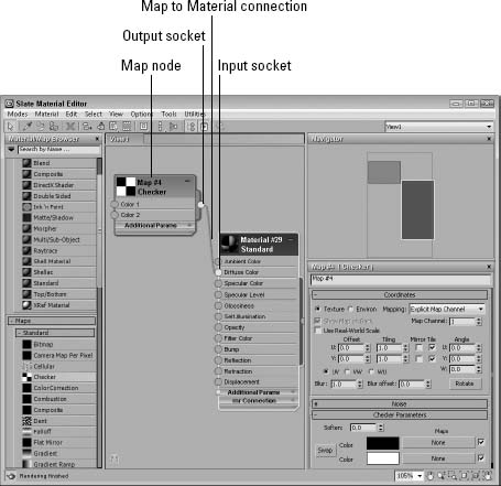
A single map node can be connected to several different material parameters on the same or on different nodes. Map nodes can also be connected to other map nodes. For example, Figure 17.3 shows a Marble and a Noise map connected to a Checker map node, which is connected to a standard material node.

FIGURE 17.3 Map nodes also can be connected to other map nodes.

To disconnect a map from a material node, simply select the connection line and press the Delete key. This removes the connection but leaves both the map and material nodes in place.

Understanding Map Types

Within the Material/Map Browser is a wide variety of different map types. Understanding these maps and their parameters enables you to create lots of different materials.

2D maps

A two-dimensional map can be wrapped onto the surface of an object or used as an environment map for a scene's background image. Because they have no depth, 2D maps appear only on the surface. The Bitmap map is perhaps the most common 2D map. It enables you to load any image, which can be wrapped around an object's surface in a number of different ways.

Many maps have several rollouts in common. These include Coordinates, Noise, and Time. In addition to these rollouts, each individual map type has its own parameters rollout.

The Coordinates rollout

Every map that is applied to an object needs to have mapping coordinates that define how the map lines up with the object. For example, with the soup can label example mentioned earlier, you probably would want to align the top edge of the label with the top edge of the can, but you could position the top edge of the map at the middle of the can. Mapping coordinates define where the map's upper-right corner is located on the object.

All map coordinates are based on a UVW coordinate system that equates to the familiar XYZ coordinate system, except that it is named uniquely so as not to be confused with transformation coordinates. For UVW coordinates, U represents the horizontal coordinate, V is the vertical coordinate, and W is along the surface normal. To keep them straight, remember that the UVW coordinate system applies to surfaces and that the XYZ coordinate system applies to spatial objects. These coordinates are required for every object to which a map is applied. In most cases, you can generate these coordinates automatically when you create an object by selecting the Generate Mapping Coordinates option in the object's Parameter rollout.

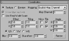
In the Coordinates rollout for 2D Maps, shown in Figure 17.4, you can specify whether the map will be a texture map or an environment map. The Texture option applies the map to the surface of an object as a texture. This texture moves with the object as the object moves. The Environ option creates an environment map. Environment maps are locked to the world and not to an object. This causes the texture to change as the object is moved. Moving an object with an environment map applied to it scrolls the map across the surface of the object.

FIGURE 17.4 The Coordinates rollout lets you offset and tile a map.

Different mapping types are available for both the Texture and Environ options. Mapping types for the Texture option include Explicit Map Channel, Vertex Color Channel, Planar from Object XYZ, and Planar from World XYZ. The Explicit Map Channel option is the default. It applies the map using the designated Map Channel. The Vertex Color Channel uses specified vertex colors as its channel. The two planar mapping types place the map in a plane based on the Local or World coordinate systems.

The Environ option includes Spherical Environment, Cylindrical Environment, Shrink-Wrap Environment, and Screen mapping types. The Spherical Environment mapping type is applied as if the entire scene were contained within a giant sphere. The same applies for the Cylindrical Environment mapping type, except that the shape is a cylinder. The Shrink-Wrap Environment plasters the map directly on the scene as if it were covering it like a blanket. All four corners of the bitmap are pulled together to the back of the wrapped object. The Screen mapping type just projects the map flatly on the background.

The Show Map on Back option causes planar maps to project through the object and be rendered on the object's back.

The U and V coordinates define the X and Y positions for the map. For each coordinate, you can specify an Offset value, which is the distance from the origin. The Tiling value is the number of times to repeat the image and is used only if the Tile option is selected. If the Use Real-World Scale option is selected, then the Offset fields change to Height and Width and the Tiling fields change to Size. The Mirror option inverts the map. The UV, VW, and WU options apply the map onto different planes.

Tiling is the process of placing a copy of the applied map next to the current one and so on until the entire surface is covered with the map placed edge to edge. You will often want to use tiled images that are seamless or that repeat from edge to edge.

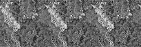
Figure 17.5 shows an image tile that is seamless. Notice how the horizontal and vertical seams line up. This figure shows three tiles positioned side by side, but because the opposite edges line up, the seams between the tiles aren't evident.

The Material Editor includes a button that you can use to check the Tiling and Mirror settings. The Sample UV Tiling button (fourth from the top) is a flyout button that you can switch to 2×2, 3×3, or 4×4.

FIGURE 17.5 Seamless image tiles are a useful way to cover an entire surface with a small map.

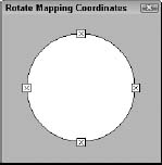
You can also rotate the map about each of the U, V, and W axes by entering values in the respective fields, or by clicking the Rotate button, which opens the Rotate Mapping Coordinates dialog box, shown in Figure 17.6. Using this dialog box, you can drag the mouse to rotate the mapping coordinates. Dragging within the circle rotates about all three coordinates, and dragging outside the circle rotates the mapping coordinates about their center point.

FIGURE 17.6 The Rotate Mapping Coordinates dialog box appears when you click the Rotate button in the Coordinates rollout.

The Blur and Blur Offset values affect the blurriness of the image. The Blur value blurs the image based on its distance from the view, whereas the Blur Offset value blurs the image regardless of its distance.

The Noise rollout

You can use the Noise rollout to randomly alter the map settings in a predefined manner. Noise can be thought of as static that you see on the television added to a bitmap. This feature is helpful for making textures more grainy, which is useful for certain materials.

The Amount value is the strength of the noise function applied; the value ranges from 0 for no noise through 100 for maximum noise. You can disable this noise function at any time, using the On option.

The Levels value defines the number of times the noise function is applied. The Size value determines the extent of the noise function based on the geometry. You can also Animate the noise. The Phase value controls how quickly the noise changes over time.

The Time rollout

Maps, such as bitmaps, that can load animations also include a Time rollout for controlling animation files. In this rollout, you can choose a Start Frame and the Playback Rate. The default Playback Rate is 1.0; higher values run the animation faster, and lower values run it slower. You also can set the animation to Loop, Ping-Pong, or Hold on the last frame.

The Output rollout

The Output rollout includes settings for controlling the final look of the map. The Invert option creates a negative version of the bitmap. The Clamp option prevents any colors from exceeding a value of 1.0 and prevents maps from becoming self-illuminating if the brightness is increased.

The Alpha From RGB Intensity option generates an alpha channel based on the intensity of the map. Black areas become transparent and white areas opaque.

The Output Amount value controls how much of the map should be mixed when it is part of a composite material. You use the RGB Offset value to increase or decrease the map's tonal values. Use the RGB Level value to increase or decrease the saturation level of the map. The Bump Amount value is used only if the map is being used as a bump map—it determines the height of the bumps.

The Enable Color Map option enables the Color Map graph at the bottom of the Output rollout. This graph displays the tonal range of the map. Adjusting this graph affects the highlights, midtones, and shadows of the map. Figure 17.7 shows a Color Map graph.

FIGURE 17.7 The Color Map graph enables you to adjust the highlights, midtones, and shadows of a map.

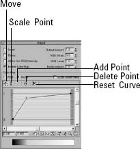
The left end of the graph equates to the shadows, and the right end is for the highlights. The RGB and Mono options let you display the graphs as independent red, green, and blue curves or as a single monocolor curve. The Copy CurvePoints option copies any existing points from Mono mode over to RGB mode, and vice versa. The buttons across the top of the graph are used to manage the graph points.

The buttons above the graph include Move (with flyout buttons for Move Horizontally and Move Vertically), Scale Point, Add Point (with a flyout button for adding a point with handles), Delete Point, and Reset Curves. Along the bottom of the graph are buttons for managing the graph view. The two fields at the bottom left contain the horizontal and vertical values for the current selected point. The other buttons are to Pan and Zoom the graph.

Bitmap map

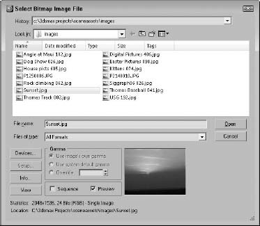
Selecting the Bitmap map from the Material/Map Browser opens the Select Bitmap Image File dialog box, shown in Figure 17.8, where you can locate an image file. Various image and animation formats are supported, including AVI, MPEG, BMP, CIN, CWS, DDF, EXR, GIF, HDRI, IFL, IPP, FLC, JPEG, MOV, PNG, PSD, RGB, RLA, RPF, TGA, TIF, and YUV.

FIGURE 17.8 The Select Bitmap Image File dialog box lets you preview images before opening them.

The name of the current bitmap file is displayed on the button in the Bitmap Parameters rollout, shown in Figure 17.9. If you need to change the bitmap file, click the Bitmap button and select the new file. Use the Reload button to update the bitmap if you've made changes to the bitmap image by an external program.

FIGURE 17.9 The Bitmap Parameters rollout offers several settings for controlling a bitmap map.

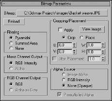
The Bitmap Parameters rollout includes three Filtering options: Pyramidal, Summed Area, and None. These methods perform a pixel-averaging operation to anti-alias the image. The Summed Area option requires more memory but produces better results.

You can also specify the output for a mono channel or for an RGB channel. For maps that use only the monochrome information in the image (such as an opacity map), the Mono Channel as RGB Intensity or Alpha option can be used. For maps that use color information (for example, a diffuse map), the RGB Channel can be RGB (full color) or Alpha as Gray.

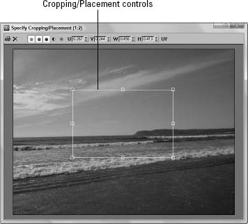
The Cropping/Placement controls enable you to crop or place the image. Cropping is the process of cutting out a portion of the image, and placing is resizing the image while maintaining the entire image and positioning it. The View Image button opens the image in a Cropping/Placement dialog box, shown in Figure 17.10. The rectangle is available within the image when Crop mode is selected. You can move the handles of this rectangle to specify the crop region.

FIGURE 17.10 Viewing an image in the Cropping/Placement dialog box enables you to set the crop marks.

You can also adjust the U and V parameters, which define the upper-left corner of the cropping rectangle, and the W and H parameters, which define the crop or placement width and height. The Jitter Placement option works with the Place option to randomly place and size the image.

If the bitmap has an alpha channel, you can specify whether it is to be used with the Image Alpha option, or you can define the alpha values as RGB Intensity or as None. You can also select to use Premultiplied Alphas. Premultiplied Alphas are images that use the transparency information stored in the image.

Checker map

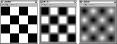
The Checker map creates a checkerboard image with two colors. The Checker Parameters rollout includes two color swatches for changing the checker colors. You can also load maps in place of each color. Use the Swap button to switch the position of the two colors and the Soften value to blur the edges between the two colors.

Figure 17.11 shows three Checker maps with Tiling values of 2 for the U and V directions and Soften values of (from left to right) 0, 0.2, and 0.5.

FIGURE 17.11 The Checker map can be softened as these three maps are with Soften values of 0, 0.2, and 0.5.

Combustion map

This map works with Autodesk's Combustion package, which is used for post-processing compositing. The Combustion map enables you to include Combustion-produced effects as a material map.

The Project button lets you load a file to paint on. These files are limited to the types that Combustion supports. Use the Edit button to load the Combustion interface.

In the Live Edit section, the Unwrap button places markings on the bitmap image to show where the mapping coordinates are located. The UV button lets you change from among UV, VW, and UW coordinate systems. The Track Time button lets you change the current frame, which enables you to paint materials that change over time. The Paint button changes the viewport cursor to enable you to paint interactively in the viewport. The Operator button lets you select a composition operator from within Combustion.

The Combustion map also includes information about current project settings for specifying a custom resolution. You can also control the Start Frame and Duration of an animation sequence. The Filtering options are Pyramidal, Summed Area, or None, and the End Conditions can be set to Loop, Ping Pong (which moves back and forth between the start and end positions), or Hold.

Gradient map

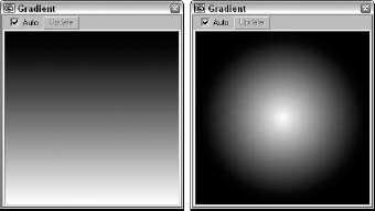
The Gradient map creates a gradient image using three colors. The Gradient Parameters rollout includes a color swatch and map button for each color. You can position the center color at any location between the two ends using the Color 2 Position value spinner. The value can range from 0 through 1. The rollout lets you choose between Linear and Radial gradient types.

The Noise Amount adds noise to the gradient if its value is nonzero. The Size value scales the noise effect, and the Phase controls how quickly the noise changes over time. The three types of noise that you can select are Regular, Fractal, and Turbulence. The Levels value determines how many times the noise function is applied. The High and Low Threshold and Smooth values set the limits of the noise function to eliminate discontinuities.

Figure 17.12 shows linear and radial Gradient maps.

FIGURE 17.12 A Gradient map can be linear (left) or radial (right).

Gradient Ramp map

This advanced version of the Gradient map can use many different colors. The Gradient Ramp Parameters rollout, shown in Figure 17.13, includes a color bar with several flags along its bottom edge. You can add flags by simply clicking along the bottom edge. You can also drag flags to reposition them or delete the interior flags by dragging them all the way to either end until they turn red.

To define the color for each flag, right-click the flag and then select Edit Properties from the pop-up menu. The Flag Properties dialog box, also shown in Figure 17.13, opens so you can select a color or texture to use.

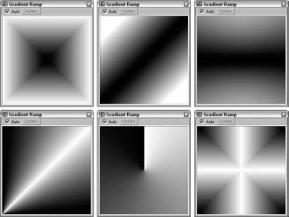
The Gradient Type drop-down in the Gradient Ramp Parameters rollout offers various Gradient Types, including 4 Corner, Box, Diagonal, Lighting, Linear, Mapped, Normal, Pong, Radial, Spiral, Sweep, and Tartan. You can also select from several Interpolation types, including Custom, Ease In, Ease In Out, Ease Out, Linear, and Solid.

FIGURE 17.13 The Flag Properties dialog box enables you to specify a color and its position to use in the Gradient Ramp.

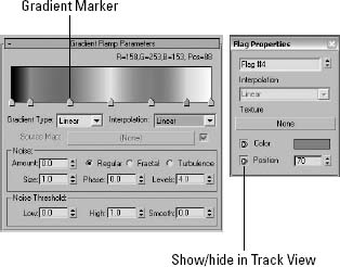
Figure 17.14 shows several of the gradient types available for the Gradient Ramp map.

FIGURE 17.14 The Gradient Ramp map offers several different gradient types, including (from top left to bottom right) Box, Diagonal, Normal, Pong, Spiral, and Tartan.

Swirl map

The Swirl map creates a swirled image of two colors: Base and Swirl. The Swirl Parameters rollout includes two color swatches and map buttons to specify these colors. The Swap button switches the two colors. Other options include Color Contrast, which controls the contrast between the two colors; Swirl Intensity, which defines the strength of the swirl color; and Swirl Amount, which is how much of the Swirl color gets mixed into the Base color.

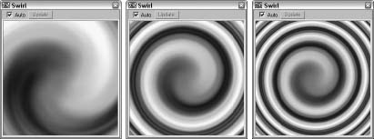
The Twist value sets the number of swirls. Negative values cause the swirl to change direction. The Constant Detail value determines how much detail is included in the swirl.

With the Swirl Location X and Y values, you can move the center of the swirl. As the center is moved far from the materials center, the swirl rings become tighter. The Lock button causes both values to change equally. If the lock is disabled, then the values can be changed independently.

The Random Seed sets the randomness of the swirl effect.

Figure 17.15 shows the Swirl map with three different Twist values. From left to right, the Twist values are 1, 5, and 10.

FIGURE 17.15 The Swirl map combines two colors in a swirling pattern.

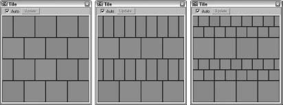
Tiles map

The Tiles map creates brick patterns. The Standard Controls rollout contains a Preset Type drop-down list with a list of preset tile patterns. These patterns are popular tile patterns including Running Bond, Common Flemish Bond, English Bond, ½ Running Bond, Stack Bond, Fine Running Bond, and Fine Stack Bond.

In the Advanced Controls rollout under both the Tile and Grout Setup sections, you can use a custom texture map and color. You can specify the Horizontal and Vertical Count of the Tiles and the Grout's Horizontal and Vertical Gaps, as well as Color and Fade Variance values for both. The Horizontal and Vertical Gaps can be locked to always be equal. For Grout, you can also define the Percentage of Holes. Holes are where tiles have been left out. A Rough value controls the roughness of the mortar.

The Random Seed value controls the randomness of the patterns, and the Swap Texture Entries option exchanges the tile texture with the grout texture.

In the Stacking Layout section, the Line Shift and Random Shift values are used to move each row of tiles a defined or random distance.

The Row and Column Editing section offers options that let you change the number of tiles Per Row or Column and the Change (or leftover) in each row or column.

Figure 17.16 shows three different Tile map styles.

FIGURE 17.16 From the Standard Controls rollout, you can select from several preset Tile styles, including Running Bond, English Bond, and Fine Running Bond.

3D maps

3D maps are procedurally created, which means that these maps are more than just a grouping of pixels; they are actually created using a mathematical algorithm. This algorithm defines the map in three dimensions, so that if a portion of the object were to be cut away, the map would line up along each edge.

The Coordinates rollout for 3D maps is similar to the Coordinates rollout for 2D maps with a few exceptions; differences include Coordinate Source options of Object XYZ, World XYZ, Explicit Map Channel, and Vertex Color Channel. There are also Offset, Tiling, and Angle values for the X-, Y-, and Z-axes as well as Blur and Blur offset options.

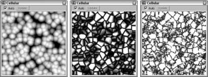
Cellular map

The Cellular 3D map creates patterns of small objects referred to as cells. In the Cell Color section of the Cellular Parameters rollout, you can specify the color for the individual cells or apply a map. Setting the Variation value can vary the cell color.

In the Division Colors section, two color swatches are used to define the colors that appear between the cells. This space is a gradient between the two colors.

In the Cell Characteristics section, you can control the shape of the cells by selecting Circular or Chips, a Size, and how the cells are Spread. The Bump Smoothing value smoothes the jaggedness of the cells. The Fractal option causes the cells to be generated using a fractal algorithm. The Iterations value determines the number of times that the algorithm is applied. The Adaptive option determines automatically the number of iterations to complete. The Roughness setting determines how rough the surfaces of the cells are.

The Size value affects the overall scale of the map, while the Threshold values specify the specific size of the individual cells. Settings include Low, Mid, and High.

Figure 17.17 shows three Cellular maps: the first with Circular cells and a Size value of 20, the second with Chips cells, and the final one with the Fractal option enabled.

FIGURE 17.17 The Cellular map creates small, regular-shaped cells.

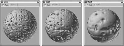
Dent map

The Dent 3D map works as a bump map to create indentations across the surface of an object. In the Dent Parameters rollout, the Size value sets the overall size of the dents. The Strength value determines how deep the dents are, and the Iterations value sets how many times the algorithm is to be computed. You can also specify the colors for the Dent map. The default colors are black and white. Black defines the areas that are indented.

Figure 17.18 shows three spheres with the Dent map applied as bump mapping. The three spheres, from left to right, have Size values of 500, 1000, and 2000.

FIGURE 17.18 The Dent map causes dents in the object when applied as bump mapping.

Falloff map

The Falloff 3D map creates a grayscale image based on the direction of the surface normals. Areas with normals that are parallel to the view are black, and areas whose normals are perpendicular to the view are white. This map is usually applied as an opacity map, giving you greater control over the opacity of the object.

The Falloff Parameters rollout includes two color swatches, a Strength value of each, and an optional map. There are also drop-down lists for setting the Falloff Type and the Falloff Direction. Falloff Types include Perpendicular/Parallel, Towards/Away, Fresnel, Shadow/Light, and Distance Blend. The Falloff Direction options include Viewing Direction (Camera Z axis); Camera X Axis; Camera Y Axis; Object; Local X, Y, and Z Axis; and World X, Y, and Z Axis.

In the Mode Specific Parameters section, several parameters are based on the Falloff Type and Direction. If Object is selected as the Falloff Direction, then a button that lets you select the object becomes active. The Fresnel Falloff Type is based on the Index of Refraction and provides an option to override the material's Index of Refraction value. The Distance Blend Falloff Type offers values for Near and Far distances.

The Falloff map also includes a Mix Curve graph and rollout that give you precise control over the falloff gradient. Points at the top of the graph have a value of 1 and represent the white areas of falloff. Points at the bottom of the graph have a value of 0 and are black.

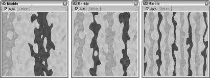
Marble map

The Marble 3D map creates a marbled material with random colored veins. The Marble Parameters rollout includes two color swatches: Color #1 is the vein color and Color #2 is the base color. You also have the option of loading maps for each color. The Swap button switches the two colors. The Size value determines how far the veins are from each other, and the Vein Width defines the vein thickness.

Figure 17.19 shows three Marble maps with Vein Width values of (from left to right) 0.01, 0.025, and 0.05.

FIGURE 17.19 The Marble map creates a marbled surface.

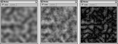
Noise map

The Noise 3D map randomly alters the surface of an object using two colors. The Noise Parameters rollout offers three Noise types: Regular, Fractal, and Turbulence. Each type uses a different algorithm for computing noise. The two color swatches let you alter the colors used to represent the noise. You also have the option of loading maps for each color. The Size value scales the noise effect. To prevent discontinuities, the High and Low Noise Threshold can be used to set noise limits.

Figure 17.20 shows Noise maps with the (from left to right) Regular, Fractal, and Turbulence options enabled.

FIGURE 17.20 The Noise map produces a random noise pattern on the surface of the object.

Particle Age map

The Particle Age map is used with particle systems to change the color of particles over their lifetime. The Particle Age Parameters rollout includes three different color swatches and age values.

Particle MBlur map

The Particle MBlur map is also used with particle systems. This map is used to blur particles as they increase in velocity. The Particle Motion Blur Parameters rollout includes two colors: The first color is the one used for the slower portions of the particle, and the second color is used for the fast portions. When you apply this map as an opacity map, the particles are blurred. The Sharpness value determines the amount of blur.

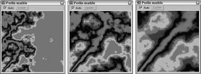
Perlin Marble map

This map creates marble textures using a different algorithm. Perlin Marble is more chaotic and random than the Marble map. The Perlin Marble Parameters rollout includes a Size parameter, which adjusts the size of the marble pattern, and a Levels parameter, which determines how many times the algorithm is applied. The two color swatches determine the base and vein colors, or you can assign a map. There are also values for the Saturation of the colors.

Figure 17.21 shows the Perlin Marble map Size values of (from left to right) 50, 100, and 200.

FIGURE 17.21 The Perlin Marble map creates a marble pattern with random veins.

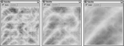
Smoke map

The Smoke map can create random fractal-based patterns such as those you would see in smoke. In the Smoke Parameters rollout, you can set the Size of the smoke areas and the number of Iterations (how many times the fractal algorithm is computed). The Phase value shifts the smoke about, and the Exponent value produces thin, wispy lines of smoke. The rollout also includes two colors for the smoke particles and the area between the smoke particles, or you can load maps instead.

Figure 17.22 shows the Smoke map with Size values of (from left to right) 40, 80, and 200.

FIGURE 17.22 The Smoke map simulates the look of smoke when applied as opacity mapping.

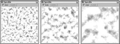
Speckle map

The Speckle map produces small, randomly positioned specks. The Speckle Parameters rollout lets you control the Size and color of the specks. Two color swatches are for the base and speck colors.

Figure 17.23 shows the Speckle map with Size values of (from left to right) 100, 200, and 400.

FIGURE 17.23 The Speckle map paints small, random specks on the surface of an object.

Splat map

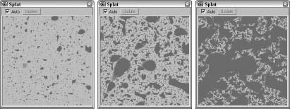
The Splat map can create the look of covering an object with splattered paint. In the Splat Parameters rollout, you can set the Size of the splattered areas and the number of Iterations, which is how many times the fractal algorithm is computed. For each additional Iteration, a smaller set of spatters appears. The Threshold value determines how much of each color to mix. The rollout also includes two colors for the splattered sections, or you can load maps instead.

Figure 17.24 shows the Splat map with a Size value of 60, 6 Iterations, and Threshold values of (from left to right) 0.2, 0.3, and 0.4.

FIGURE 17.24 The Splat map splatters paint randomly across the surface of an object.

Stucco map

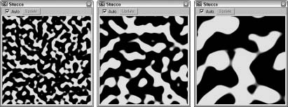
The Stucco map generates random patches of gradients that create the look of a stucco surface if applied as a bump map. In the Stucco Parameters rollout, the Size value determines the size of these areas. The Thickness value determines how blurry the patches are, which changes the sharpness of the bumps for a bump map. The Threshold value determines how much of each color to mix. The rollout also includes two colors for the patchy sections, or you can load maps instead.

Figure 17.25 shows the Stucco map with a Threshold value of 0.5, Thickness of 0.02, and Size values of (from left to right) 10, 20, and 40.

FIGURE 17.25 The Stucco map creates soft indentations when applied as bump mapping.

Waves map

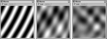
This map creates wavy, watery-looking maps and can be used as both a diffuse map and a bump map to create a water surface. You can use several values to set the wave characteristics in the Water Parameters rollout, including the number of Wave Sets, the Wave Radius, the minimum and maximum Wave Length, the Amplitude, and the Phase. You can also Distribute the waves as 2D or 3D, and a Random Seed value is available.

Figure 17.26 shows the Water map with the Num Wave Sets value set to (from left to right) 1, 3, and 9.

FIGURE 17.26 You can use the Water map to create watery surfaces.

Wood map

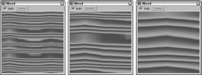
The Wood map produces a two-color wood grain. The Wood Parameters rollout options include Grain Thickness, Radial, and Axial Noise. You can select the two colors to use for the wood grain.

Figure 17.27 shows the Wood map with Grain Thickness values of (from left to right) 8, 16, and 30.

FIGURE 17.27 The Wood map creates a map with a wood grain.

Compositor maps

Compositor maps are made by combining several maps into one. Compositor map types include Composite, Mask, Mix, and RGB Multiply.

Composite map

Composite maps combine a specified number of maps into a single map using the alpha channel. Each separate map is listed on a separate layer, and the layers are composited from the top layer down. The Composite Parameters rollout lists the number of layers and includes a button for adding a new layer, as shown in Figure 17.28.

Each layer has preview swatches for specifying a texture and a mask. To the side of these preview swatches are buttons for hiding the layer or mask and for color correcting each. There are also buttons for deleting, renaming, and duplicating each layer.

FIGURE 17.28 The Composite Layers rollout lists each composite map as a separate layer.

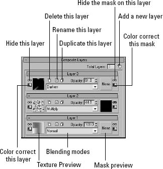
The Opacity value sets how transparent the layer is, and you can also change the blending mode using the drop-down list at the bottom of each layer. The blending mode defines how the texture on the current layer is combined with the layers below it. The available blending modes include Normal, Average, Addition, Subtract, Darken, Multiply, Color Burn, Linear Burn, Lighten, Screen, Color Dodge, Linear Dodge, Spotlight, Spotlight Blend, Overlay, Soft Light, Hard Light, Pinlight, Hard Mix, Difference, Exclusion, Hue, Saturation, Color, and Value.

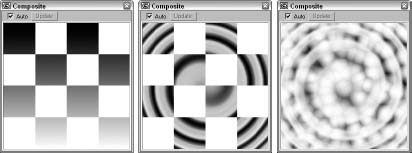
Figure 17.29 shows three different uses for the Composite map. The left image combines a Checker map with a Gradient map. The last two images combine a Swirl map with Checker and Cellular maps.

FIGURE 17.29 The Composite map can use multiple maps.

Mask map

In the Mask Parameters rollout, you can select one map to use as a Mask and another one to display through the holes in the mask simply called Map. You also have an option to Invert the Mask. The black areas of the masking map are the areas that hide the underlying map. The white areas allow the underlying map to show through. The result of the Mask map is visible only when rendered.

Mix map

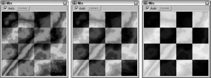
You can use the Mix map to combine two maps or colors. It is similar to the Composite map, except that it uses a Mix Amount value to combine the two colors or maps instead of using the alpha channel. In the Mix Parameters rollout, the Mix Amount value of 0 includes only Color #1, and a value of 100 includes only Color #2. You can also use a Mixing Curve to define how the colors are mixed. The curve shape is controlled by altering its Upper and Lower values.

Figure 17.30 shows the Mix map with Perlin Marble and Checker maps applied as sub-maps and Mix values of (from left to right) 25, 50, and 75.

FIGURE 17.30 The Mix map lets you combine two maps and define the Mix Amount.

RGB Multiply map

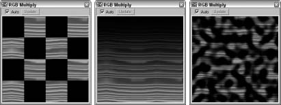
The RGB Multiply map multiplies the RGB values for two separate maps and combines them to create a single map. Did you notice in the preceding figure that the Mix map fades both maps? The RGB Multiply map keeps the saturation of the individual maps by using each map's alpha channel to combine the maps.

The RGB Multiply Parameters rollout includes an option to use the Alpha from either Map #1 or Map #2 or to Multiply the Alphas.

Figure 17.31 shows three samples of the RGB Multiply map. Each of these images combines a Wood map with (from left to right) a Checker map, a Gradient map, and a Stucco map. Notice that the colors aren't faded for this map type.

FIGURE 17.31 The RGB Multiply map combines maps at full saturation using alpha channels.

Color Modifier maps

You can use this group of maps to change the color of different materials. Color Modifier map types include Output, RGB Tint, and Vertex Color.

Color Correction map

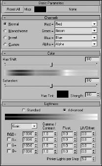
The Color Correction map lets you change the colors of a texture. The corrections are applied using a stack approach. The Color Correction map includes four rollouts: Basic Parameters, Channels, Color, and Lightness, as shown in Figure 17.32, and each of these settings is in order starting from the top rollout.

The Basic Parameters rollout includes a color swatch and a map button that you can use to specify the color to affect the map. In the Channels rollout, you can select to make the map Normal, Monochrome, Invert, or Custom. If Custom is selected, then you can specify a specific color for each of the RGB and alpha channels. The available channel options are Red, Green, Blue, Alpha, the inverse for each, Monochrome, One, and Zero.

In the Color rollout, you can adjust the Hue Shift, Saturation, Hue Tint, and Strength for the map, and the Lightness rollout gives you two options: Standard and Advanced. In Standard mode, you can adjust the Brightness and Contrast using simple sliders, but Advanced mode gives you control over the Gain, F-Stops, and Printer Lights settings for each channel.

FIGURE 17.32 The Color Correction map lets you work with textures as if you had a photo lab.

Output map

The Output map provides a way to add the functions of the Output rollout to maps that don't include an output rollout. Details on this map type are presented in the earlier section that covers the Output rollout.

RGB Tint map

The RGB Tint map includes color swatches for the red, green, and blue channel values. Adjusting these colors alters the amount of tint in the map. For example, setting the red color swatch in the RGB Tint Parameters rollout to white and the green and blue color swatches to black creates a map with a heavy red tint. You can also load maps in place of the colors.

Vertex Color map

The Vertex Color map makes the vertex colors assigned to an Editable Mesh, Poly, or Patch object visible when the object is rendered. When an Editable Mesh, Poly, or Patch object is in Vertex subobject mode, you can assign the selected vertices a Color, an Illumination color, and an Alpha value. These settings are in the Surface Properties rollout. You can also assign vertex colors using the Assign Vertex Colors utility. Use this utility to assign color to the current object or to assign material colors to the object's vertices using the given lights. A third way to assign vertex colors is with the Vertex Paint modifier, which you access using the Modifiers Mesh Editing Vertex Paint menu command. This modifier lets you color vertices by painting directly on an object.

After vertex colors are assigned, you need to apply the Vertex Color map to the diffuse color in the Material Editor and apply it to the object for the object to render the vertex colors. This map doesn't have any settings.

Miscellaneous maps

These maps are actually grouped into a category called Other, but they mostly deal with reflection and refraction effects. Maps in this category include Camera Map Per Pixel, Flat Mirror, Normal Bump, Raytrace, Reflect/Refract, and Thin Wall Refraction.

Camera Map Per Pixel map

The Camera Map Per Pixel map lets you project a map from the location of a camera. You use this map by rendering the scene, editing the rendered image in an image-editing program, and projecting the image back onto the scene.

The Camera Map Parameters rollout includes buttons that let you select the Camera, Texture, ZBuffer Mask, and Mask.

Flat Mirror map

The Flat Mirror map reflects the surroundings using a coplanar group of faces. In the Flat Mirror Parameters rollout, you can select a Blur amount to apply. You can specify whether to Render the First Frame Only or Every Nth Frame. You also have an option to Use the Environment Map or to apply to Faces with a given ID.

The Distortion options include None, Use Bump Map, and Use Built-In Noise. If the Bump Map option is selected, you can define a Distortion Amount. If the Noise option is selected, you can choose Regular, Fractal, or Turbulence noise types with Phase, Size, and Levels values.

Tutorial: Creating a mirrored surface

Mirror, mirror on the wall, who's the best modeler of them all? Using the Flat Mirror map, you can create, believe it or not, mirrors. To create and configure a flat mirror map, follow these steps:

1. Open the Reflection in mirror.max file from the Chap 17 directory on the CD.

   This file includes a mesh of a man standing in front of a mirror. The mirror subobject faces have been selected and applied a material ID of 1.

2. Choose Rendering Material Editor Slate Material Editor (or press the M key) to open the Material Editor.
3. Locate and double-click the Flat Mirror option in the Material/Map Browser to add a node to the Node View. Drag a connection wire from the output socket, drop it anywhere on the Node View, and then select the Materials/Standard material from the pop-up menu and the Reflection channel from the parameters pop-up menu. This adds a standard material node to the Node View and connects the Flat Mirror node to the material's Reflection parameter.

   Note

   If the Flat Mirror map isn't available, select the Map radio button in the Show section.

4. Double-click the Flat Mirror node to make its parameters appear in the Parameter Editor. In the Flat Mirror Parameters rollout, deselect the Apply Blur and Use Environment Map options and select the Apply to Faces with ID option. Then set the ID value to 1.
5. Drag the material node's output socket to the mirror object in the viewport to apply the material to the mirror.

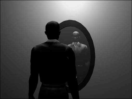
Figure 17.33 shows a model being reflected off a simple patch object with a Flat Mirror map applied to it. The reflection is visible only in the final rendered image.

FIGURE 17.33 A Flat Mirror map causes the object to reflect its surroundings.

Normal Bump map

The Normal Bump map lets you alter the appearance of the details on the surface using a Normal map. Normal maps can be created using the Render to Texture dialog box. The Parameters rollout for this map type lets you specify a normal map along with another additional bump map. You also can set the amount each map is displaced. Additional options let you flip and swap the red and green channel directions, which define the X and Y axes.

Raytrace map

The Raytrace map is an alternative to the raytrace material and, as a map, can be used in places where the raytrace material cannot.

Reflect/Refract map

Reflect/Refract maps are yet another way to create reflections and refractions on objects. These maps work by producing a rendering from each axis of the object, like one for each face of a cube. These rendered images, called cubic maps, are then projected onto the object.

These rendered images can be created automatically or loaded from pre-rendered images using the Reflect/Refract Parameters rollout. Using automatic cubic maps is easier, but they take considerably more time. If you select the Automatic option, you can select to render the First Frame Only or Every Nth Frame. If you select the From File option, then you are offered six buttons that can load cubic maps for each of the different directions.

In the Reflect/Refract Parameters rollout, you can also specify the Blur settings and the Atmospheric Ranges.

Thin Wall Refraction map

The Thin Wall Refraction map simulates the refraction caused by a piece of glass, such as a magnifying glass. The same result is possible with the Reflect/Refract map, but the Thin Wall Refraction map achieves this result in a fraction of the time.

The Thin Wall Refraction Parameters rollout includes options for setting the Blur, the frames to render, and Refraction values. The Thickness Offset determines the amount of offset and can range from 0 through 10. The Bump Map Effect value changes the refraction based on the presence of a bump map.

Tutorial: Creating a magnifying glass effect

Another common property of glass besides reflection is refraction. Refraction can enlarge items when the glass is thick, such as when you look at the other side of the room through a glass of water. Using the Thin Wall Refraction map, you can simulate the effects of a magnifying glass.

To create a magnifying glass effect, follow these steps:

1. Open the Magnifying glass.max file from the Chap 17 directory on the CD.

   This file includes a simple sphere with a Perlin Marble map applied to it and a magnifying glass modeled from primitive objects.

2. Choose Rendering Material Editor Slate Material Editor (or press the M key) to open the Material Editor.
3. Locate and double-click the Thin Wall Refraction option in the Material/Map Browser to add a node to the Node View. Drag a connection wire from the output socket, drop it anywhere on the Node View, and then select the Materials/Standard material from the pop-up menu and the Refraction channel from the parameters pop-up menu. This adds a standard material node to the Node View and connects the Thin Wall Refraction node to the material's Reflection parameter.
4. Double-click the Thin Wall Refraction node to open its parameters in the Parameter Editor. In the Thin Wall Refraction Parameters rollout, set the Thickness Offset to 10 to increase the amount of magnification.
5. Drag the output socket for the material node and drop it on the magnifying glass object in the viewport to apply the material to the object.

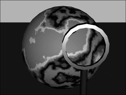
Figure 17.34 shows the resulting rendered image. Notice that the texture in the magnifying glass appears magnified.

FIGURE 17.34 The Thin Wall Refraction map is applied to a magnifying glass.

Using the Maps Rollout

Now that you've seen the different types of maps, we'll revisit the Maps rollout (introduced in Chapter 15), shown in Figure 17.35, and cover it in more detail.

The Maps rollout is where you apply maps to the various materials. To use a map, click the Map button; this opens the Material/Map Browser where you can select the map to use. The Amount spinner sets the intensity of the map, and an option to enable or disable the map is available. For example, a white diffuse color with a red Diffuse map set at 50 percent Intensity results in a pink material.

The available maps in the Maps rollout depend on the type of material and the Shader that you are using. Raytrace materials have many more available maps than the standard material. Some of the common mapping types found in the Maps rollout are discussed in Table 17.1.

FIGURE 17.35 The Maps rollout can turn maps on or off.

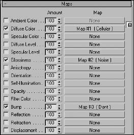
TABLE 17.1 Material Properties for Maps

Material Property	Description
Ambient Color	Replaces the ambient color component of the base material. You can use this feature to make an object's shadow appear as a map. Diffuse mapping (discussed next) also affects the Ambient color. A lock button in the Maps rollout enables you to lock these two mappings together.
Diffuse Color	Replaces the diffuse color component of the base material. This is the main color used for the object. When you select a map such as Wood, the object appears to be created out of wood. As mentioned previously, diffuse mapping also can affect the Ambient color if the lock button is selected.
Diffuse Level	Changes the diffuse color level from 0, where the map is black, to a maximum, where the map is white. This mapping is available only with the Anisotropic, Oren-Nayar-Blinn, and Multi-Level Shaders.
Diffuse Roughness	Sets the roughness value of the material from 0, where the map is black, to a maximum, where the map is white. This mapping is available only with the Oren-Nayar-Blinn and Multi-Layer Shaders.
Specular Level	Controls the intensity of the specular highlights from 0, where the map is black, to 1, where the map is white. For the best effect, apply this mapping along with the Glossiness mapping.
Glossiness	Defines where the specular highlights will appear. You can use this option to make an object appear older by diminishing certain areas. Black areas on the map show the non-glossy areas, and white areas are where the glossiness is at a maximum.
Opacity	Determines which areas are visible and which are transparent. Black areas for this map are transparent, and white areas are opaque. This mapping works in conjunction with the Opacity value in the Basic Parameters rollout. Transparent areas, even if perfectly transparent, still receive specular highlights.
Filter Color	Colors transparent areas for creating materials such as colored glass. White light that is cast through an object using filter color mapping is colored with the filter color.
Anisotropy	Controls the shape of an anisotropy highlight. This mapping is available only with the Anisotropic and Multi-Layer Shaders.
Orientation	Controls an anisotropic highlight's position. Anisotropic highlights are elliptical, and this mapping can position them at a different angle. Orientation mapping is available only with the Anisotropic and Multi-Layer Shaders.
Metalness	Controls how metallic an area looks. It specifies metalness values from 0, where the map is black, to a maximum, where the map is white. This mapping is available only with the Strauss Shader.
Bump	Uses the intensity of the bitmap to raise or indent the surface of an object. The white areas of the map are raised, and darker areas are lowered. Although bump mapping appears to alter the geometry, it actually doesn't affect the surface geometry.
Reflection	Reflects images off the surface as a mirror does. The three types of Reflection mapping are Basic, Automatic, and Flat Mirror. Basic reflection mapping simulates the reflection of an object's surroundings. Automatic reflection mapping projects the map outward from the center of the object. Flat-Mirror reflection mapping reflects a mirror image off a series of coplanar faces. Reflection mapping doesn't need mapping coordinates because the coordinates are based on world coordinates and not on object coordinates. Therefore, the map appears different if the object is moved, which is how reflections work in the real world.
Refraction	Bends light and displays images through a transparent object, in the same way a room appears through a glass of water. The amount of this effect is controlled by a value called the Index of Refraction. This value is set in the parent material's Extended Parameters rollout.
Displacement	Changes the geometry of an object. The white areas of the map are pushed outward, and the dark areas are pushed in. The amount of the surface displaced is based on a percentage of the diagonal that makes up the bounding box of the object. Displacement mapping isn't visible in the viewports unless the Displace NURBS (for NURBS, or Non-Uniform Rational B-Splines, objects) or the Displace Mesh (for Editable Meshes) modifiers have been applied.

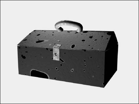
Tutorial: Aging objects for realism

I don't know whether your toolbox is well worn like mine—it must be the hostile environment that it is always in (or all the things I keep dropping in and on it). Rendering a toolbox with nice specular highlights just doesn't feel right. This tutorial shows a few ways to age an object so that it looks older and worn.

To add maps to make an object look old, follow these steps:

1. Open the Toolbox.max file from the Chap 17 directory on the CD.

   This file contains a simple toolbox mesh created using extruded splines.

2. Press the M key to open the Slate Material Editor. Locate and double-click the Standard material in the Material/Map Browser, and then select the Metal shader from the drop-down list in the Shader Basic Parameters rollout. In the Metal Basic Parameters rollout, set the Diffuse color to a nice, shiny red and increase the Specular Level to 97 and the Glossiness value to 59. Name the material Toolbox.
3. In the Maps rollout of the Material/Map Browser, double-click the option for the Splat map and connect this node to the Glossiness parameter. In the Splat Parameters rollout, set the Size value to 100 and change Color #1 to a rust color and Color #2 to white.
4. Double-click the Dent option in the Material/Map Browser and connect its node to the Bump parameter. Select the Dent map node and in the Dent Parameters rollout, set the Size value to 200, Color #1 to black, and Color #2 to white.
5. Create another standard material node and name it Hinge. Select the Metal shader from the Shader Basic Parameters rollout for this material also, and increase the Specular Level in the Metal Basic Parameters rollout to 26 and the Glossiness value to 71. Also change the Diffuse color to a light gray. Click the map button next to the Glossiness value, and double-click the Noise map in the Material/Map Browser. In the Noise Parameters rollout, set the Noise map to Fractal with a Size of 10.
6. Drag the output socket for the “Toolbox” material to the toolbox object and the “Hinge” material to the hinge and the handle.

Figure 17.36 shows the well-used toolbox.

FIGURE 17.36 This toolbox shows its age with Glossiness and Bump mappings.

Using the Map Path Utility

After you have all your maps in place, losing them can really make life troublesome. However, Max includes a utility that helps you determine which maps are missing and lets you edit the path to them to quickly and easily locate them. The Bitmap/Photometric Path Editor utility is available in the Utility panel. To find it, click the More button and select Bitmap/Photometric Path Editor from the list of utilities.

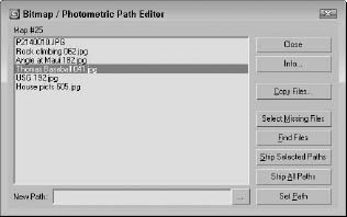
When opened, the Path Editor rollout includes the Edit Resources button that opens the Bitmap/Photometric Path Editor window, shown in Figure 17.37. The rollout also includes two options for displaying the Materials Editor and Material Library bitmap paths. The Close button closes the rollout.

The Info button in the Bitmap/Photometric Path Editor dialog box lists all the nodes that use the selected map. The Copy Files button opens a File dialog box in which you can select a location to which to copy the selected map. The Select Missing Files button selects any maps in the list that can't be located. The Find Files button lists the maps in the current selection that can be located and the number that are missing. Stripping paths removes the path information and leaves only the map name. The New Path field lets you enter the path information to apply to the selected maps. The button with three dots to the right of the New Path field lets you browse for a path, and the Set Path button applies the path designated in the New Path field to the selected maps.

FIGURE 17.37 The Bitmap/Photometric Path Editor window lets you alter map paths.

Using Map Instances

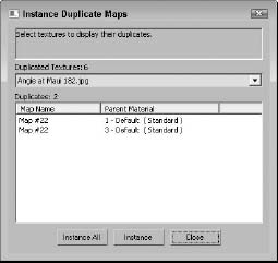
Using the same bitmap for many different map channels is common. For example, you may use the same bitmap for the Diffuse and Bump map channels. If a file includes the same bitmaps over and over, the file size can increase, and replacing a bitmap when you make changes can become difficult. This potential problem can be fixed easily by making the maps into instances instead of copies. If you have an existing Max file, you can use the Instance Duplicate Maps utility to find all the common maps and make them instances automatically.

Access this utility from the Utilities menu in the Material Editor or from the Utilities panel. Both commands open the same dialog box, shown in Figure 17.38. From this dialog box, you can select which maps to make instances or click Instance All to consolidate all the found maps into instances.

FIGURE 17.38 The Instance Duplicate Maps dialog box lets you consolidate maps into a single instance.

Creating Textures with External Tools

Several external tools can be valuable when you create material textures. These tools can include an image-editing program like Photoshop, a digital camera or camcorder, and a scanner. With these tools, you can create or capture images that can be applied as maps to a material using the map channels.

After the image is created or captured, you can apply it to a material by clicking a map shortcut button or by selecting a map in the Maps rollout. This opens the Material/Map Browser, where you can select the Bitmap map type and load the image file from the File dialog box that appears.

Creating material textures using Photoshop

When you begin creating texture images, Photoshop becomes your best friend. Using Photoshop's filters enables you to quickly create a huge variety of textures that add life and realism to your textures.

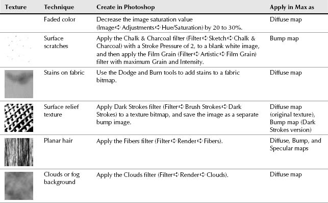
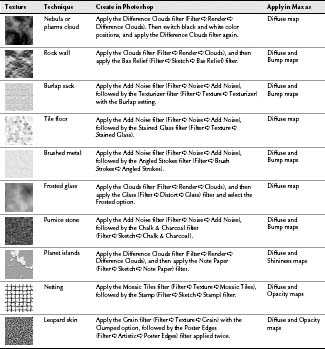
Table 17.2 is a recipe book of several common textures that you can create in Photoshop. The table provides only a quick sampling of some simple textures. Many other features and effects are possible with Photoshop.

TABLE 17.2 Photoshop Texture Recipes

Capturing digital images

Digital cameras and camcorders are inexpensive enough that they really are necessary items when creating material textures. Although Photoshop can be used to create many unique and interesting textures, a digital image of riverbed stones is much more realistic than anything that can be created with Photoshop. The world is full of interesting textures that can be used when creating images.

Avoiding specular highlights

Nothing can ruin a good texture taken with a digital camera faster than the camera's flash. Taking a picture of a highly reflective surface like the surface of a table can reflect back to the camera, thereby ruining the texture.

You can counter this several ways. One technique is to block the flash and make sure that you have enough ambient light to capture the texture. Taking pictures outside can help with this because they don't need the flash. Another technique is to take the image at an angle, but this might skew the texture. A third technique is to take the image and then crop away the unwanted highlights.

Adjusting brightness

Digital images that are taken with a digital camera are typically pre-lit, meaning that they already have a light source lighting them. When these pre-lit images are added to a Max scene that includes lights, the image gets a double dose of light that typically washes out the images.

You can remedy this problem by adjusting the brightness of the image prior to loading it into Max. For images taken in normal indoor light, you'll want to decrease the brightness value by 10 to 20 percent. For outdoor scenes in full sunlight, you may want to decrease the brightness even more.

You can find the Brightness/Contrast control in Photoshop in the Image Adjustments Brightness/Contrast menu.

Scanning images

In addition to taking digital images with a digital camera, you can scan images from other sources. For example, the maple leaf modeled using patches in Chapter 13, “Modeling with Polygons,” was scanned from a real leaf found in my yard.

When scanning images, use the scanner's descreen option to remove any dithering from the printed image. If you place the image on a piece of matte black construction paper, then the internal glare from the scanning bulb gets a more uniform light distribution.

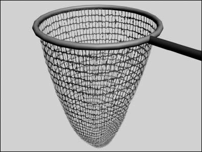
Tutorial: Creating a fishing net

Some modeling tasks can be solved more easily with a material than with geometry changes. A fishing net is a good example. Using geometry to create the holes in the net would be tricky, but a simple Opacity map makes this complex modeling task easy.

To create a fishing net, follow these steps:

1. Before working in Max, create the needed texture in Photoshop. In Photoshop, select File New, enter the dimensions of 512 pixels × 512 pixels in the New dialog box, and click OK to create a new image file.
2. Select the Filter Texture Mosaic Tiles menu command to apply the Mosaic Tiles filter. Set the Tile Size to 30 and the Grout Width to 3, and click OK. Then select the Filter Sketch Stamp menu command to apply the Stamp filter with a Light/Dark Balance value of 49 and a Smooth value of 50.
3. Choose File Save As, and save the file as Netting.tif.

   A copy of this file is available in the Chap 17 directory on the CD.

4. Open the Fish net.max file from the Chap 17 directory on the CD.

   This file includes a fishing net model created by stretching half a sphere with the Shell modifier applied.

5. Select the Rendering Material Editor Slate Material Editor menu command (or press the M key) to open the Material Editor. Double-click the Standard option in the Material/Map Browser to create a material node. Name the material net.
6. Locate and double-click the Bitmap option in the Material/Map Browser to add a node to the Node View. In the File dialog box that opens, locate and select the netting.tif image file. Drag a connection wire from the output socket of the Bitmap node and drop it on the input node of the Opacity parameter of the material node. Then drag the output socket for the material node and drop it on the net object in the viewports.
7. If you were to render the viewport, the net would look rather funny because the black lines are transparent instead of the white spaces. To fix this, select the Bitmap node, open the Output rollout, and enable the Invert option. This inverts the texture image.

Figure 17.39 shows the rendered net.

FIGURE 17.39 A fishing net, completed easily with the net texture applied as an Opacity map

Summary

We've covered lots of ground in this chapter because Max has lots of different maps. Learning to use these maps will make a big difference in the realism of your materials.

In this chapter, you learned about the following:

• Connecting map nodes in the Slate Material Editor to material nodes.
• All the different map types in several different categories, including 2D, 3D, Compositors, Color Mods, and Reflection/Refraction
• The various mapping possibilities provided in the Maps rollout
• Using the Bitmap Path Editor to change map paths
• Using the Duplicate Map Instances utility
• How to create materials using external tools such as Photoshop and a digital camera

By combining materials and maps, you can create an infinite number of material combinations, but Max has even more ways to build and apply materials. In the next chapter, you learn how complex materials and material modifiers are used.