
Channel Estimation, Equalization, Precoding, and Tracking
Jitendra K. Tugnait, Department of Electrical and Computer Engineering, Auburn University, Auburn, AL, USA
Abstract
We present an overview/review of various approaches to channel estimation and equalization for wireless mobile systems with a brief discussion of channel precoding techniques. Since approaches to channel estimation depend upon the underlying channel model, we also review various approaches to channel modeling. First we present the relevant channel models including time-invariant and time-variant (doubly-selective) models where emphasis is on basis expansion modeling. Channel modeling is followed by a discussion of various approaches to channel estimation including training-based approaches, blind approaches, semi-blind approaches and hidden pilot (superimposed training) based approaches. Channel estimation approaches were followed by a discussion of channel equalization approaches including turbo-equalization for time-varying channels. A brief discussion of precoding was presented where the channel state information is available at the transmitter. We conclude with a discussion of channel tracking and combined data detection and channel tracking for time-varying channels. Channel tracking can be at block level suitable for block transmissions, or symbol-by-symbol level suitable for serial transmissions. Some of the approaches were illustrated via simulations.
Keywords
Channel estimation; Basis expansion channel models; Equalization; Adaptive equalizers; Turbo equalization; Maximum likelihood; Channel tracking; Precoding
2.03.1 Introduction
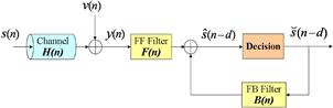
Multipath propagation results in a received signal that is a superposition of several delayed and scaled copies of the transmitted signal giving rise to frequency-selective fading. It leads to intersymbol interference (ISI) at the receiver which, in turn, may lead to high error rates in symbol detection. Equalizers are designed to compensate for these channel distortions. One may directly design an equalizer given the received signal, or one may first estimate the channel impulse response and then design an equalizer based on the estimated channel. After some processing (matched filtering, for instance), the continuous-time received signals are sampled at the baud (symbol) or higher (fractional) rate before processing them for channel estimation and/or equalization. It is therefore convenient to work with a baseband-equivalent discrete-time channel model. Depending upon the sampling rate, one has either a single-input single-output (SISO) (baud rate sampling), or a single-input multiple-output (SIMO) (fractional sampling), complex discrete-time equivalent baseband channel. Knowledge of the channel response can be advantageously used at the transmitter to precode the information sequence to be transmitted so as to simplify the equalizer complexity at the receiver and to mitigate interference in MIMO systems.
In this chapter, we present an overview/review of various approaches to channel estimation and equalization for wireless mobile systems with a brief discussion of channel precoding techniques. Since approaches to channel estimation depend upon the underlying channel model, we also review various approaches to channel modeling. In Section 2.03.2 we present the relevant channel models including time-variant and time-invariant models. In Section 2.03.3 various channel estimation methods are discussed. In Section 2.03.4 equalization approaches are reviewed and in Section 2.03.5 a brief discussion of precoding approaches is presented. In Section 2.03.6 we discuss tracking to adapt to time-varying channels.
Notation 1
Superscripts ![]() , and
, and ![]() denote the complex conjugate transpose, complex conjugation, transpose, and Moore-Penrose pseudo-inverse operations, respectively. The function
denote the complex conjugate transpose, complex conjugation, transpose, and Moore-Penrose pseudo-inverse operations, respectively. The function ![]() is the Kronecker delta function with
is the Kronecker delta function with ![]() if
if ![]() otherwise, and
otherwise, and ![]() is the
is the ![]() identity matrix. The symbol
identity matrix. The symbol ![]() denotes the Kronecker product, and
denotes the Kronecker product, and ![]() is the trace of a square matrix
is the trace of a square matrix ![]() . The
. The ![]() th entry of a matrix
th entry of a matrix ![]() is denoted by
is denoted by ![]() .
.
2.03.2 Channel models
2.03.2.1 Time-variant (doubly selective) channels
Consider a time-varying (e.g., mobile wireless) channel (linear system) with complex baseband, continuous-time, received signal ![]() and transmitted complex baseband, continuous-time information signal
and transmitted complex baseband, continuous-time information signal ![]() (with symbol interval
(with symbol interval ![]() seconds) related by [1]
seconds) related by [1]
![]() (3.1)
(3.1)
where ![]() is the time-varying impulse response of the channel denoting the response of the channel at time t to a unit impulse input at time
is the time-varying impulse response of the channel denoting the response of the channel at time t to a unit impulse input at time ![]() and
and ![]() is the additive noise (typically white Gaussian). A delay-Doppler spread function
is the additive noise (typically white Gaussian). A delay-Doppler spread function ![]() is defined as the Fourier transform of
is defined as the Fourier transform of ![]() with respect to t [1,2]
with respect to t [1,2]
![]() (3.2)
(3.2)
If ![]() for
for ![]() , then
, then ![]() is called the (multipath) delay-spread of the channel. If
is called the (multipath) delay-spread of the channel. If ![]() for
for ![]() , then
, then ![]() is called the Doppler spread of the channel. In order to capture the complexity of the physical interactions characterizing the transmission through a real channel,
is called the Doppler spread of the channel. In order to capture the complexity of the physical interactions characterizing the transmission through a real channel, ![]() is typically modeled as a two-dimensional zero-mean random process. If
is typically modeled as a two-dimensional zero-mean random process. If ![]() is wide-sense stationary in variable t, and
is wide-sense stationary in variable t, and ![]() is uncorrelated with
is uncorrelated with ![]() for
for ![]() and any t, one obtains the well-known wide-sense stationary uncorrelated scattering (WSSUS) channel [1,2, Chapter 14].
and any t, one obtains the well-known wide-sense stationary uncorrelated scattering (WSSUS) channel [1,2, Chapter 14].
2.03.2.1.1 Tapped delay line model
We now consider a discrete-time channel model. If a linear modulation scheme is used, the baseband transmitted signal can be represented as
![]() (3.3)
(3.3)
where ![]() is the information sequence and
is the information sequence and ![]() is the transmit (lowpass) filter (typically a root raised cosine filter). Therefore, the baseband signal at the receiver is given by
is the transmit (lowpass) filter (typically a root raised cosine filter). Therefore, the baseband signal at the receiver is given by
![]() (3.4)
(3.4)
After filtering with a receive filter with impulse response ![]() , the received baseband signal is given by
, the received baseband signal is given by
![]() (3.5)
(3.5)
where ![]() . If the continuous-time signal
. If the continuous-time signal ![]() is sampled at once every
is sampled at once every ![]() sec., we obtain the discrete-time sequence
sec., we obtain the discrete-time sequence
![]() (3.6)
(3.6)
where ![]() is the (effective) channel response at time n to a unit impulse input at time
is the (effective) channel response at time n to a unit impulse input at time ![]() and
and
![]() (3.7)
(3.7)
Note that the noise sequence ![]() in (3.6) is no longer necessarily white; it can be whitened by further time-invariant linear filtering (see [1]). Henceforth, we assume that a whitening filter has been applied to
in (3.6) is no longer necessarily white; it can be whitened by further time-invariant linear filtering (see [1]). Henceforth, we assume that a whitening filter has been applied to ![]() , but with an abuse of notation, we will still use (3.6). For a causal system,
, but with an abuse of notation, we will still use (3.6). For a causal system, ![]() for
for ![]() (
(![]() ) and for a finite length channel of maximum length
) and for a finite length channel of maximum length ![]() for
for ![]() (
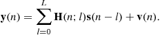
(![]() ). In this case we modify (3.6) as (recall the noise whitening filter)
). In this case we modify (3.6) as (recall the noise whitening filter)
 (3.8)
(3.8)
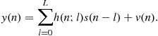
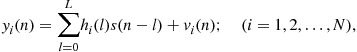
The model (3.8) represents a time- and frequency-selective linear channel. A tapped delay line structure for this model is shown in Figure 3.1. For a slowly (compared to the baud-rate) time-varying system, one often simplifies (3.8) to a time-invariant system as
 (3.9)
(3.9)
where ![]() is the time-invariant channel response to a unit impulse input at time 0. The model (3.9) represents a frequency-selective linear channel with no time selectivity. It is a widely used model for receiver design.
is the time-invariant channel response to a unit impulse input at time 0. The model (3.9) represents a frequency-selective linear channel with no time selectivity. It is a widely used model for receiver design.
Figure 3.1 Tapped delay line model of frequency- and time-selective channel with finite impulse response. D represents a unit (symbol duration) delay.
Suppose that ![]() . Then we have the time-selective and frequency-nonselective channel whose output is given by
. Then we have the time-selective and frequency-nonselective channel whose output is given by
![]() (3.10)
(3.10)
Finally, a time-nonselective and frequency-nonselective channel is modeled as
![]() (3.11)
(3.11)
where h is a random variable (or a constant).
2.03.2.1.2 Autoregressive (AR) models
It is possible to accurately represent a wide-sense stationary uncorrelated scattering (WSSUS) channel by a large order AR model; see [3–5] and references therein. Let
![]() (3.12)
(3.12)
where ![]() is
is ![]() vector. Then a pth order AR model, AR(p), for
vector. Then a pth order AR model, AR(p), for ![]() is given by
is given by
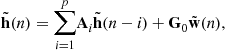 (3.13)
where ![]() s are the
s are the ![]() AR coefficient matrices,
AR coefficient matrices, ![]() is also
is also ![]() and independent and identically distributed (i.i.d.),
and independent and identically distributed (i.i.d.), ![]() driving noise
driving noise ![]() is zero-mean with identity covariance matrix. Suppose that we know the correlation function
is zero-mean with identity covariance matrix. Suppose that we know the correlation function ![]() for lags
for lags ![]() . The following Yule-Walker equation holds for (3.13) [6]:
. The following Yule-Walker equation holds for (3.13) [6]:
 (3.14)
Using (3.14) for ![]() , and the fact that
, and the fact that ![]() , one can estimate
, one can estimate ![]() s. Using the estimated
s. Using the estimated ![]() s and (3.14) for
s and (3.14) for ![]() , one can find
, one can find ![]() , from which one can find (non-unique)
, from which one can find (non-unique) ![]() by computing its “square root” [7, p. 358]. In [3] high values of p (several tens) have been used for channel simulation, whereas in [4,5] only AR(1) or AR(2) models have been used where the objective is channel estimation and related issues. An AR(1) model is given by
by computing its “square root” [7, p. 358]. In [3] high values of p (several tens) have been used for channel simulation, whereas in [4,5] only AR(1) or AR(2) models have been used where the objective is channel estimation and related issues. An AR(1) model is given by
![]() (3.15)
(3.15)
where ![]() is the AR coefficient, and the driving noise
is the AR coefficient, and the driving noise ![]() is zero-mean complex Gaussian with variance
is zero-mean complex Gaussian with variance ![]() and statistically independent of
and statistically independent of ![]() . Assume that
. Assume that ![]() is also zero-mean, complex Gaussian with variance
is also zero-mean, complex Gaussian with variance ![]() . Then [8]
. Then [8]
![]() (3.16)
(3.16)
2.03.2.1.3 Basis expansion models
Basis expansion models (BEMs) have also been widely investigated to represent doubly selective channels in wireless applications [9–13], where the time-varying taps are expressed as superpositions of time-varying basis functions in modeling Doppler effects, weighted by time-invariant coefficients. Candidate basis functions include complex exponential (Fourier) functions [10,11], polynomials [9], and discrete prolate spheroidal sequences [13], etc. In contrast to AR models that describe temporal variation on a symbol-by-symbol update basis, a BEM depicts the evolution of the channel over a period (block) of time. Intuitively, the coefficients of the BEM approximation should evolve much more slowly in time than the channel, and hence are more convenient to track in a fast fading environment.
Suppose that we include the effects of transmit and receive filters in the time-variant impulse response ![]() in (3.1). Suppose that this channel has a delay-spread
in (3.1). Suppose that this channel has a delay-spread ![]() and a Doppler spread
and a Doppler spread ![]() . Consider the kth block of data consisting of an observation window of
. Consider the kth block of data consisting of an observation window of ![]() symbols where the baud-rate data samples in the block are indexed as
symbols where the baud-rate data samples in the block are indexed as ![]() . If
. If ![]() (underspread channel), the complex exponential basis expansion model (CE-BEM) representation of
(underspread channel), the complex exponential basis expansion model (CE-BEM) representation of ![]() in (3.8) is given by
in (3.8) is given by
 (3.17)
where one chooses (![]() , and K is an integer)
, and K is an integer)
![]() (3.18)
(3.18)
![]() (3.19)
(3.19)
The BEM coefficients ![]() s remain invariant during this block, but are allowed to change at the next block, and the Fourier basis functions
s remain invariant during this block, but are allowed to change at the next block, and the Fourier basis functions ![]() (
(![]() ) are common for each block. If the delay spread
) are common for each block. If the delay spread ![]() and the Doppler spread
and the Doppler spread ![]() of the channel (or at least their upper-bounds) are known, one can infer the basis functions of the CE-BEM [11]. Treating the basis functions as known, estimation of a time-varying process is reduced to estimating the invariant coefficients over a block of length
of the channel (or at least their upper-bounds) are known, one can infer the basis functions of the CE-BEM [11]. Treating the basis functions as known, estimation of a time-varying process is reduced to estimating the invariant coefficients over a block of length ![]() symbols. Note that the BEM period is
symbols. Note that the BEM period is ![]() whereas the block size is
whereas the block size is ![]() symbols. If
symbols. If ![]() (e.g.,
(e.g., ![]() or
or ![]() ), then the Doppler spectrum is said to be over-sampled [14] compared to the case
), then the Doppler spectrum is said to be over-sampled [14] compared to the case ![]() where the Doppler spectrum is said to be critically sampled. In [10,11] only
where the Doppler spectrum is said to be critically sampled. In [10,11] only ![]() (henceforth called CE-BEM) is considered whereas [14] considers
(henceforth called CE-BEM) is considered whereas [14] considers ![]() (henceforth called over-sampled CE-BEM).
(henceforth called over-sampled CE-BEM).
Equation (3.17) applies to single-input single-output systems—one user and one receiver with symbol-rate sampling. It is easily modified to handle multiuser, multiple transmit and receive antennas, and higher than symbol rate sampling (multiple samples per symbol)—the basic representation remains essentially unchanged.
The representation ![]() in (3.17) is a special case of a more general representation
in (3.17) is a special case of a more general representation
 (3.20)
where ![]() are a set of orthogonal basis functions (over the time interval under consideration). Examples include wavelet-based expansions as in [15], polynomial bases as in [9] and other possibilities [16]. In discrete prolate spheroidal BEM (DPS-BEM), the ith DPS vector
are a set of orthogonal basis functions (over the time interval under consideration). Examples include wavelet-based expansions as in [15], polynomial bases as in [9] and other possibilities [16]. In discrete prolate spheroidal BEM (DPS-BEM), the ith DPS vector
![]()
(called Slepian sequence in [13], which is a time-windowed (infinite) DPS sequence) is the ith eigenvector of a matrix ![]() [17]:
[17]:
![]()
is the ![]() th entry of
th entry of ![]() and
and ![]() are the eigenvalues of
are the eigenvalues of ![]() . The Slepian sequences
. The Slepian sequences ![]() are orthonormal over the finite time interval
are orthonormal over the finite time interval ![]() . The modeling error of the CE-BEM can result in a noticeable floor in BER curves [18]. The polynomial basis functions are neither time-limited nor band-limited and their square bias varies heavily over the range of Doppler spread considered in [13]. DPS sequences are a good alternative as a basis set to approximate bandlimited channels alleviating the spectral leakage of CE-BEM [13]. The (infinite) DPS sequences have their maximum energy concentration in an interval with length T while being bandlimited to
. The modeling error of the CE-BEM can result in a noticeable floor in BER curves [18]. The polynomial basis functions are neither time-limited nor band-limited and their square bias varies heavily over the range of Doppler spread considered in [13]. DPS sequences are a good alternative as a basis set to approximate bandlimited channels alleviating the spectral leakage of CE-BEM [13]. The (infinite) DPS sequences have their maximum energy concentration in an interval with length T while being bandlimited to ![]() , where
, where ![]() is the unique sequence that is bandlimited and most time-concentrated,
is the unique sequence that is bandlimited and most time-concentrated, ![]() is the next sequence having maximum energy concentration among the DPS sequences orthogonal to
is the next sequence having maximum energy concentration among the DPS sequences orthogonal to ![]() , and so on [17].
, and so on [17].
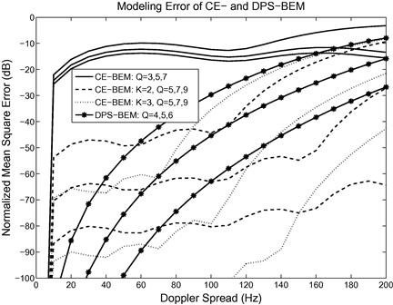
Figure 3.2 shows the channel modeling errors resulting from (critically sampled) CE-BEM, DPS-BEM and oversampled CE-BEM (![]() or 3) when the underlying channel is a one-tap time-selective channel following Jakes’ spectrum. The results are based on Monte Carlo averaging over 1000 runs with
or 3) when the underlying channel is a one-tap time-selective channel following Jakes’ spectrum. The results are based on Monte Carlo averaging over 1000 runs with ![]() and varying Doppler spreads. (The results were obtained following the procedure in [13].) For a fixed value of Q, DPS-BEM provides the best fit whereas CE-BEM (no oversampling) yields minor improvements with increasing Q. On the other hand, the basis functions in oversampled CE-BEM are not mutually orthogonal leading to “analytical” difficulties. There exists a vast literature based on CE-BEM (no oversampling) where it is assumed that physical channel is accurately described by CE-BEM both for analysis and simulations; see e.g., [11,19–24].
and varying Doppler spreads. (The results were obtained following the procedure in [13].) For a fixed value of Q, DPS-BEM provides the best fit whereas CE-BEM (no oversampling) yields minor improvements with increasing Q. On the other hand, the basis functions in oversampled CE-BEM are not mutually orthogonal leading to “analytical” difficulties. There exists a vast literature based on CE-BEM (no oversampling) where it is assumed that physical channel is accurately described by CE-BEM both for analysis and simulations; see e.g., [11,19–24].
2.03.2.2 Time-invariant channels
For a baud (symbol)-rate sampled system, the equivalent baseband channel model is given by (3.9) which is a single-input single-output (SISO) complex discrete-time baseband-equivalent channel model. The output sequence ![]() in (3.9) is discrete-time stationary. When there is excess channel bandwidth [bandwidth
in (3.9) is discrete-time stationary. When there is excess channel bandwidth [bandwidth ![]() (baud rate)], baud rate sampling is below the Nyquist rate leading to aliasing and depending upon the symbol timing phase, in certain cases, causing deep spectral notches in sampled, aliased channel transfer function [25]. Linear equalizers designed on the basis of the baud-rate sampled channel response, are quite sensitive to symbol timing errors. Initially, in the trained case, fractional sampling was investigated to robustify the equalizer performance against timing errors. The model (3.9) does not apply to fractionally-spaced samples, i.e., when the sampling interval is a fraction of the symbol duration. The fractionally sampled digital communication signal is a cyclostationary signal [26] which may be represented as a vector stationary sequence using a time series representation (TSR) ([26] Section 12.6). Suppose that we sample at N-times the baud rate with signal samples spaced
(baud rate)], baud rate sampling is below the Nyquist rate leading to aliasing and depending upon the symbol timing phase, in certain cases, causing deep spectral notches in sampled, aliased channel transfer function [25]. Linear equalizers designed on the basis of the baud-rate sampled channel response, are quite sensitive to symbol timing errors. Initially, in the trained case, fractional sampling was investigated to robustify the equalizer performance against timing errors. The model (3.9) does not apply to fractionally-spaced samples, i.e., when the sampling interval is a fraction of the symbol duration. The fractionally sampled digital communication signal is a cyclostationary signal [26] which may be represented as a vector stationary sequence using a time series representation (TSR) ([26] Section 12.6). Suppose that we sample at N-times the baud rate with signal samples spaced ![]() sec. apart where
sec. apart where ![]() is the symbol duration. Then a TSR for the sampled signal is given by
is the symbol duration. Then a TSR for the sampled signal is given by
 (3.21)
where now we have N samples every symbol period, indexed by i. Notice, however, that the information sequence ![]() is still one “sample” per symbol. It is assumed that the signal incident at the receiver is first passed through a receive filter whose transfer function equals the square root of a raised cosine pulse, and that the receive filter is matched to the transmit filter. The noise sequence in (3.21) is the result of the fractional rate sampling of a filtered continuous-time white Gaussian noise process. Therefore, the sampled noise sequence is white at the symbol rate, but correlated at the fractional rate. Stack N consecutive received samples in the nth symbol duration to form a N-vector
is still one “sample” per symbol. It is assumed that the signal incident at the receiver is first passed through a receive filter whose transfer function equals the square root of a raised cosine pulse, and that the receive filter is matched to the transmit filter. The noise sequence in (3.21) is the result of the fractional rate sampling of a filtered continuous-time white Gaussian noise process. Therefore, the sampled noise sequence is white at the symbol rate, but correlated at the fractional rate. Stack N consecutive received samples in the nth symbol duration to form a N-vector ![]() satisfying
satisfying
 (3.22)
where ![]() is the vector impulse response of the SIMO equivalent channel model given by
is the vector impulse response of the SIMO equivalent channel model given by
![]() (3.23)
(3.23)
2.03.2.3 MIMO channels
A general MIMO channel model with K inputs (users, antennas, ![]() ) and N outputs (receivers, antennas,
) and N outputs (receivers, antennas, ![]() ) can be formulated as in (3.48) (given later); however, it lacks “physical” parameters (such as antenna spacing and arrangement). Representative works on MIMO channel models that incorporate “propagation” effects include [27–31] and references therein. The Kronecker model of [30] is a popular analytical model for spatially-correlated MIMO channels. It models the correlation at the receiver and at the transmitter independently, neglecting the statistical interdependence of both link ends. Improvements upon this model include the virtual channel representation model of [29] and the stochastic model of [31] where joint correlation at both link ends have been considered and experimentally validated. These models are suitable for wireless local area networks (WLANs). For wireless personal area networks (WPANs), a different MIMO channel model has been proposed in [28] to account for irregular (nonuniform) antenna arrangements and other deviations.
) can be formulated as in (3.48) (given later); however, it lacks “physical” parameters (such as antenna spacing and arrangement). Representative works on MIMO channel models that incorporate “propagation” effects include [27–31] and references therein. The Kronecker model of [30] is a popular analytical model for spatially-correlated MIMO channels. It models the correlation at the receiver and at the transmitter independently, neglecting the statistical interdependence of both link ends. Improvements upon this model include the virtual channel representation model of [29] and the stochastic model of [31] where joint correlation at both link ends have been considered and experimentally validated. These models are suitable for wireless local area networks (WLANs). For wireless personal area networks (WPANs), a different MIMO channel model has been proposed in [28] to account for irregular (nonuniform) antenna arrangements and other deviations.
2.03.3 Channel estimation
We first consider three types of channel estimators within the framework of maximizing the likelihood function. [Unless otherwise noted the underlying channel model is given by the time-invariant model (3.22).] In general, one of the most effective and popular parameter estimation algorithms is the maximum likelihood (ML) method.
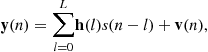
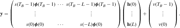
Let us consider the N-vector channel model given in (3.22). Suppose that we have collected M samples of the observation ![]() . We then have the following linear model
. We then have the following linear model
 (3.24)
where ![]() is an
is an ![]() identity matrix,
identity matrix, ![]() and
and ![]() are vectors consisting of samples of the input sequence
are vectors consisting of samples of the input sequence ![]() and noise
and noise ![]() , respectively,
, respectively, ![]() is the vector of the channel parameters, and a block Hankel matrix has identical block entries on its block antidiagonals. Let
is the vector of the channel parameters, and a block Hankel matrix has identical block entries on its block antidiagonals. Let ![]() be the vector of unknown parameters that may include the channel parameters
be the vector of unknown parameters that may include the channel parameters ![]() and possibly the entire or part of the input vector
and possibly the entire or part of the input vector ![]() . Given the probability space that describes jointly the noise vector
. Given the probability space that describes jointly the noise vector ![]() and possibly the input data vector
and possibly the input data vector ![]() , we can then obtain, in principle, the probability density function (pdf) of the observation
, we can then obtain, in principle, the probability density function (pdf) of the observation ![]() . As a function of the unknown parameter
. As a function of the unknown parameter ![]() , the pdf of the observation
, the pdf of the observation ![]() is referred to as the likelihood function. The maximum likelihood estimator is defined by the following optimization
is referred to as the likelihood function. The maximum likelihood estimator is defined by the following optimization
![]() (3.25)
(3.25)
where ![]() defines the domain of the optimization.
defines the domain of the optimization.
While the ML estimator is conceptually simple, and it usually has good performance when the sample size is sufficiently large, the implementation of ML estimator is sometimes computationally intensive. Furthermore, the optimization of the likelihood function in (3.25) is often hampered by the existence of local maxima. Therefore, it is desirable that effective initialization techniques are used in conjunction with the ML estimation.
2.03.3.1 Training-based channel estimation
The training-based channel estimation assumes the availability of the input vector ![]() (as training symbols) and its corresponding observation vector
(as training symbols) and its corresponding observation vector ![]() . When the noise samples are zero mean, white Gaussian, i.e.,
. When the noise samples are zero mean, white Gaussian, i.e., ![]() is a zero mean, Gaussian random vector with covariance
is a zero mean, Gaussian random vector with covariance ![]() , the ML estimator defined in (3.25), with
, the ML estimator defined in (3.25), with ![]() , is given by
, is given by
![]() (3.26)
(3.26)
where ![]() is the Moore-Penrose pseudo-inverse of the
is the Moore-Penrose pseudo-inverse of the ![]() defined in (3.24). This is also the classical linear least-squares estimator which can be implemented recursively, and it turns out to be the best (in terms of having minimum mean square error) among all unbiased estimators and it is the most efficient in the sense that it achieves the Cramer-Rao lower bound. Various adaptive implementations can be found in [1].
defined in (3.24). This is also the classical linear least-squares estimator which can be implemented recursively, and it turns out to be the best (in terms of having minimum mean square error) among all unbiased estimators and it is the most efficient in the sense that it achieves the Cramer-Rao lower bound. Various adaptive implementations can be found in [1].
2.03.3.1.1 Time-variant channels
In case of general time-varying channels represented by (3.6), a simple generalization of [32] (see also [11]) is to use a periodic Kronecker delta function sequence with period ![]() as training:
as training:
![]() (3.27)
(3.27)
With (3.27) as input to model (3.6), one obtains
![]() (3.28)
(3.28)
so that if ![]() , we have for
, we have for ![]() ,
,
![]() (3.29)
(3.29)
Therefore, one may take the estimate of ![]() as
as
![]() (3.30)
(3.30)
For time samples between ![]() (k an integer), linear interpolation may be used to obtain channel estimates.
(k an integer), linear interpolation may be used to obtain channel estimates.
If we use the BEM representation (3.20), then we directly estimate the time-invariant parameters ![]() s. From (3.6) and (3.20) we have
s. From (3.6) and (3.20) we have
 (3.31)
 (3.32)
Collecting ![]() samples of the observations
samples of the observations ![]() we have the linear model
we have the linear model
 (3.33)
Now we have a model similar to (3.24) with a solution similar to (3.26).
2.03.3.2 Blind channel estimation
Here no training symbols are available (or exploited). Blind techniques can not resolve phase ambiguity in the channel estimate.
2.03.3.2.1 Combined channel and symbol estimation
The simultaneous estimation of the input vector and the channel is general ill-posed; however, utilization of qualitative information about the channel and the input can help alleviate this deficiency. To this end, we consider two different types of maximum likelihood techniques based on different models of the input sequence.
Stochastic Maximum Likelihood Estimation. While the input vector ![]() is unknown, it may be modeled as a random vector with a known distribution. In such a case, the likelihood function of the unknown parameter
is unknown, it may be modeled as a random vector with a known distribution. In such a case, the likelihood function of the unknown parameter ![]() (cf. (3.24)) can be obtained by
(cf. (3.24)) can be obtained by
![]() (3.34)
(3.34)
where ![]() is the marginal pdf of the input vector and
is the marginal pdf of the input vector and ![]() is the likelihood function when the input is known. Assume, for example, that the input data symbol
is the likelihood function when the input is known. Assume, for example, that the input data symbol ![]() takes, with equal probability, a finite number (
takes, with equal probability, a finite number (![]() ) of values. Consequently, the input data vector
) of values. Consequently, the input data vector ![]() also takes values from the signal set
also takes values from the signal set ![]() . The likelihood function of the channel parameters is then given by
. The likelihood function of the channel parameters is then given by
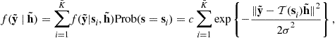 (3.35)
where c is a constant, ![]() , and the stochastic maximum likelihood estimator is given by
, and the stochastic maximum likelihood estimator is given by
 (3.36)
The maximization of the likelihood function defined in (3.34) is in general difficult because ![]() is non-convex. The Expectation-Maximization (EM) algorithm can be applied to transform the complicated optimization to a sequence of quadratic optimizations. Kaleh and Vallet [33] first applied the EM algorithm to the equalization of communication channels with input sequence having finite alphabet property. By using a Hidden Markov Model (HMM), they developed a batch (off-line) procedure that includes the so-called forward and backward recursions. The complexity of this algorithm increases exponentially with the channel memory.
is non-convex. The Expectation-Maximization (EM) algorithm can be applied to transform the complicated optimization to a sequence of quadratic optimizations. Kaleh and Vallet [33] first applied the EM algorithm to the equalization of communication channels with input sequence having finite alphabet property. By using a Hidden Markov Model (HMM), they developed a batch (off-line) procedure that includes the so-called forward and backward recursions. The complexity of this algorithm increases exponentially with the channel memory.
To relax the memory requirements and facilitate channel tracking, “on-line” sequential approaches have been proposed in [34] for input with finite alphabet properties under a HMM formulation. Given the appropriate regularity conditions and a good initialization guess, it can be shown that these algorithms converge to the true channel value.
Deterministic Maximum Likelihood Estimation. The deterministic ML approach assumes no statistical model for the input sequence ![]() . In other words, both the channel vector
. In other words, both the channel vector ![]() and the input source vector
and the input source vector ![]() are parameters to be estimated. When the noise is zero-mean Gaussian with covariance
are parameters to be estimated. When the noise is zero-mean Gaussian with covariance ![]() , the ML estimates can be obtained by the nonlinear least squares optimization
, the ML estimates can be obtained by the nonlinear least squares optimization
![]() (3.37)
(3.37)
The joint minimization of the likelihood function with respect to both the channel and the source parameter spaces is difficult. Fortunately, the observation vector ![]() is linear in both the channel and the input parameters individually. In particular, we have
is linear in both the channel and the input parameters individually. In particular, we have
![]() (3.38)
(3.38)
where
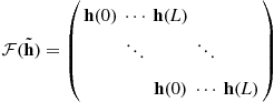 (3.39)
is the so-called filtering matrix. We therefore have a separable nonlinear least squares problem that can be solved sequentially
![]() (3.40)
(3.40)
If we are only interested in estimating the channel, the above minimization can be rewritten as
 (3.41)
where ![]() is a projection transform of
is a projection transform of ![]() into the orthogonal complement of the range space of
into the orthogonal complement of the range space of ![]() , or the noise subspace of the observation, and
, or the noise subspace of the observation, and ![]() denotes the pseudo-inverse of
denotes the pseudo-inverse of ![]() . Discussions of algorithms of this type can be found in [35].
. Discussions of algorithms of this type can be found in [35].
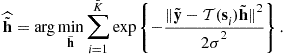
Similar to the HMM for statistical maximum likelihood approach, the finite alphabet properties of the input sequence can also be incorporated into the deterministic maximum likelihood methods. These algorithms, first proposed by Seshadri [36] and Ghosh and Weber [37], iterate between estimates of the channel and the input. At iteration k, with an initial guess of the channel ![]() , the algorithm estimates the input sequence
, the algorithm estimates the input sequence ![]() and the channel
and the channel ![]() for the next iteration by
for the next iteration by
![]() (3.42)
(3.42)
![]() (3.43)
(3.43)
where ![]() is the (discrete) domain of
is the (discrete) domain of ![]() . The optimization in (3.43) is a linear least squares problem whereas the optimization in (3.42) can be achieved by using the Viterbi algorithm [1]. Seshadri [36] presented blind trellis search techniques. Reduced-state sequence estimation was proposed in [37]. Raheli et al. proposed a per-survivor processing technique in [38]. The convergence of such approaches is not guaranteed in general. Interesting examples have been provided in [39] where two different combinations of
. The optimization in (3.43) is a linear least squares problem whereas the optimization in (3.42) can be achieved by using the Viterbi algorithm [1]. Seshadri [36] presented blind trellis search techniques. Reduced-state sequence estimation was proposed in [37]. Raheli et al. proposed a per-survivor processing technique in [38]. The convergence of such approaches is not guaranteed in general. Interesting examples have been provided in [39] where two different combinations of ![]() and
and ![]() lead to the same cost
lead to the same cost ![]() .
.
2.03.3.2.2 The methods of moments
Although the ML channel estimator discussed in Section 2.03.3.2.1 usually provides better performance, the computation complexity and the existence of local optima are the two major difficulties. Therefore, “simpler” approaches have also been investigated.
SISO Channel Estimation. For baud-rate data, second-order statistics of the data do not carry enough information to allow estimation of the channel impulse response as a typical channel is nonminimum-phase. On the other hand, higher order statistics (in particular, fourth-order cumulants) of the baud-rate (or fractional rate) data can be exploited to yield the channel estimates to within a scale factor. Given the mathematical model (3.9), there are two broad classes of direct approaches to channel estimation, the distinguishing feature among them being the choice of the optimization criterion. All of the approaches involve (more or less) a least-squares error measure. The error definition differs, however, as follows:
• Fitting error: Match the model-based higher-order (typically fourth-order) statistics to the estimated (data-based) statistics in a least-squares sense to estimate the channel impulse response, as in [40,41], for example. This approach allows consideration of noisy observations. In general, it results in a nonlinear optimization problem. It requires availability of a good initial guess to prevent convergence to a local minimum. It yields estimates of the channel impulse response.
• Equation error: It is based on minimizing an “equation error” in some equation which is satisfied ideally. The approaches of [42,43] (among others) fall in this category. In general, this class of approaches results in a closed-form solution for the channel impulse response so that a global extremum is always guaranteed provided that the channel length (order) is known. These approaches may also provide good initial guesses for the nonlinear fitting error approaches. Quite a few of these approaches fail if the channel length is unknown.
Further details may be found in [44] and references therein.
SIMO Channel Estimation. Here we will concentrate upon second-order statistical methods. For single-input multiple-output vector channels the autocorrelation function of the observation is sufficient for the identification of the channel impulse response up to an unknown constant [45,46], provided that the various subchannels have no common zeros. This observation led to a number of techniques under both statistical and deterministic assumptions of the input sequence [35]. By exploiting the multichannel aspects of the channel (e.g., crosscorrelation among the outputs of various subchannels), many of these techniques lead to a constrained quadratic optimization
![]() (3.44)
(3.44)
where ![]() is a positive definite matrix constructed from the observation. Asymptotically (either as the sample size increases to infinity or the noise variance approaches to zero), these estimates converge to true channel parameters.
is a positive definite matrix constructed from the observation. Asymptotically (either as the sample size increases to infinity or the noise variance approaches to zero), these estimates converge to true channel parameters.
2.03.3.3 Semi-blind approaches
Semi-blind approaches utilize a combination of training-based and blind approaches. Here we present a brief discussion about the idea and refer the reader to the survey [47] for details. The objective of semi-blind channel estimation (and equalization) is to exploit the information used by blind methods as well as the information exploited by the training-based methods. Semi-blind channel estimation assumes additional knowledge of the input sequence. Specifically, part of the input data vector is known. Both the statistical and deterministic maximum likelihood estimators remain the same except that the likelihood function needs to be modified to incorporate the knowledge of the input. However, semi-blind channel estimation may offer significant performance improvement over either the blind or the training based methods as demonstrated in the evaluation of Cramer-Rao lower bound in [47].
There are many generalizations of blind channel estimation techniques to incorporate known symbols. In [48], Tsatsanis and Cirpan extended the approach of Kaleh and Vallet by restricting the transition of hidden Markov model. In [49], the knowledge of the known symbol is used to avoid the local maxima in the maximization of the likelihood function. A popular approach is to combine the objective function used to derive blind channel estimator with the least squares cost in the training-based channel estimation. For example, a weighted linear combination of the cost for blind channel estimator and that for the training based estimator can be used [50,51].
2.03.3.4 Superimposed training-based approaches
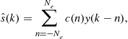
In the superimposed training (hidden pilots) based approach, one takes
![]() (3.45)
(3.45)
where ![]() is the information sequence and
is the information sequence and ![]() is a non-random periodic training (pilot) sequence. Exploitation of the periodicity of
is a non-random periodic training (pilot) sequence. Exploitation of the periodicity of ![]() allows identification of the channel without allocating any explicit time slots for training, unlike traditional training methods. There is no loss in data transmission rate. On the other hand, some useful power is wasted in superimposed training which could have otherwise been allocated to the information sequence. This lowers the effective signal-to-noise ratio (SNR) for the information sequence and affects the bit error rate (BER) at the receiver.
allows identification of the channel without allocating any explicit time slots for training, unlike traditional training methods. There is no loss in data transmission rate. On the other hand, some useful power is wasted in superimposed training which could have otherwise been allocated to the information sequence. This lowers the effective signal-to-noise ratio (SNR) for the information sequence and affects the bit error rate (BER) at the receiver.
Superimposed training-based approaches have been discussed in [52–54] for SISO systems. A block transmission method has been proposed in [55,56] where a data-dependent component is added to the superimposed training such that interference due to data (information sequence) is greatly reduced in channel estimation at the receiver. This method is applicable to time-invariant channels only and it requires “data-blocking” for block transmissions and insertion of a cyclic prefix in each data block. Its extension to a class of time-variant channels is given in [57]; see also [58]. The UTRA specification for 3G systems [59] allows to adopt a spread pilot (superimposed) sequence in the base station’s common pilot channel, which is suitable for downlinks. Periodic superimposed training for channel estimation via first-order statistics for SISO systems have been discussed in [60–63]. In [64] performance bounds for training and superimposed training-based semiblind SISO channel estimation for time-varying flat fading channels have been discussed.
2.03.3.5 MIMO channel estimation
All of the channel estimation approaches described earlier apply to MIMO channels; however, efficacy of the approaches depends upon the underlying analytical model used. For MIMO channel estimation in correlated fading enviroments, Chen and su [27] presents two analytical MIMO channel models and low-complexity iterative channel estimation methods based on these models, exploiting the optimal training sequences proposed in [65,66]. Further details may be found in these papers and references therein.
2.03.4 Equalization
A communication channel is typically modeled as a linear system whose output is corrupted by additive noise. Equalizers are designed to compensate for channel distortions as well as noise. One may directly design an equalizer given the received signal, or one may first estimate the channel impulse response and then design an equalizer based on the estimated channel. The structure of the equalizer is dictated by channel models, computational complexity and possible exchange of information with a channel (error correction) decoder.
2.03.4.1 Linear equalization
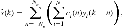
The most common channel equalizer structure is a linear transversal filter. Given model (3.9) for the baud-rate sampled received signal, the linear transversal equalizer output ![]() is an estimate of
is an estimate of ![]() given by
given by
 (3.46)
where ![]() are the
are the ![]() -tap weight (equalizer) coefficients of the
-tap weight (equalizer) coefficients of the ![]() -tap equalizer. Two criteria have found widespread use in optimizing the equalizer coefficients: peak distortion criterion and mean-square error (MSE) criterion. Under the MSE criterion one chooses
-tap equalizer. Two criteria have found widespread use in optimizing the equalizer coefficients: peak distortion criterion and mean-square error (MSE) criterion. Under the MSE criterion one chooses ![]() s to minimize
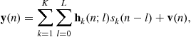
s to minimize ![]() . Linear equalizers designed on the basis of the baud-rate sampled received signal are quite sensitive to symbol timing errors [25]. Therefore, fractionally-spaced linear equalizers (typically with twice the baud-rate sampling: oversampling by a factor of two) are quite widely used to mitigate sensitivity to symbol timing errors. A fractionally spaced equalizer (FSE) in the linear transversal structure has the output
. Linear equalizers designed on the basis of the baud-rate sampled received signal are quite sensitive to symbol timing errors [25]. Therefore, fractionally-spaced linear equalizers (typically with twice the baud-rate sampling: oversampling by a factor of two) are quite widely used to mitigate sensitivity to symbol timing errors. A fractionally spaced equalizer (FSE) in the linear transversal structure has the output
 (3.47)
where ![]() are the
are the ![]() tap weight coefficients of the ith sub-equalizer. Note that the FSE outputs data at the symbol rate. Various criteria and cost functions exist to design the linear equalizers in both batch and recursive (adaptive) form [1, Chapters 10, 14].
tap weight coefficients of the ith sub-equalizer. Note that the FSE outputs data at the symbol rate. Various criteria and cost functions exist to design the linear equalizers in both batch and recursive (adaptive) form [1, Chapters 10, 14].
For time-varying channels the equalizer coefficients ![]() or
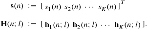
or ![]() in (3.46) and (3.47), respectively, are also functions of k. An alternative is to use either a BEM-based equalizer with time-invariant equalizer coefficients coupled with time-varying exponential basis function [67] or a Kalman fixed-lag smoother (Kalman Detector) [68]. To illustrate the Kalman detector, consider a multi-input multi-output (MIMO) channel with K inputs (users, antennas,
in (3.46) and (3.47), respectively, are also functions of k. An alternative is to use either a BEM-based equalizer with time-invariant equalizer coefficients coupled with time-varying exponential basis function [67] or a Kalman fixed-lag smoother (Kalman Detector) [68]. To illustrate the Kalman detector, consider a multi-input multi-output (MIMO) channel with K inputs (users, antennas, ![]() ) and N outputs (receivers, antennas,
) and N outputs (receivers, antennas, ![]() ); one can adapt this easily to single-input single-output (SISO) or single-input multi-output (SIMO) systems. Let
); one can adapt this easily to single-input single-output (SISO) or single-input multi-output (SIMO) systems. Let ![]() denote kth user’s information sequence that is input to the time-varying channel with discrete-time response
denote kth user’s information sequence that is input to the time-varying channel with discrete-time response ![]() (channel response for the kth user at time instance n to a unit input at time instance
(channel response for the kth user at time instance n to a unit input at time instance ![]() ). We assume that
). We assume that ![]() s are mutually independent and identically distributed (i.i.d.) with zero mean and variance
s are mutually independent and identically distributed (i.i.d.) with zero mean and variance ![]() for
for ![]() . Then, at symbol-rate sampling, the noisy N-column channel output vector is given by (
. Then, at symbol-rate sampling, the noisy N-column channel output vector is given by (![]() )
)
 (3.48)
where the N-column vector ![]() is zero-mean, white, uncorrelated with
is zero-mean, white, uncorrelated with ![]() , complex Gaussian noise, with the autocorrelation
, complex Gaussian noise, with the autocorrelation ![]() . Define
. Define
Then we may rewrite (3.48) as
 (3.49)
2.03.4.1.1 Kalman detector (KD)
The Kalman filter, together with a quantizer, acts as the symbol detector at the receiver end. The state and the measurement equations are given by
![]() (3.50)
(3.50)
![]() (3.51)
(3.51)
with the following definitions

where ![]() is K-column vector of symbols (data or training),
is K-column vector of symbols (data or training), ![]() is the known or estimated
is the known or estimated ![]() channel matrix and integer
channel matrix and integer ![]() (it will also be the equalization delay). Assume data symbols are zero-mean and white. If
(it will also be the equalization delay). Assume data symbols are zero-mean and white. If ![]() is a data symbol, we have
is a data symbol, we have ![]() and
and ![]() ; if
; if ![]() is a training symbol,
is a training symbol, ![]() and
and ![]() .
.
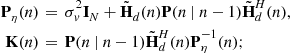
Kalman filtering for the system described by (3.50) and (3.51) is initialized with
![]()
where ![]() denotes the estimate of
denotes the estimate of ![]() given the observations
given the observations ![]() , and
, and ![]() denotes the error covariance matrix of
denotes the error covariance matrix of ![]() , defined as
, defined as
![]()
Then recursive filtering (for ![]() ) is applied via the following steps:
) is applied via the following steps:

The estimated state vector is given by
![]()
and we extract its last (K-column vector) term ![]() as the desired equalized output for K-users with equalization delay d. Finally, we hard-quantize
as the desired equalized output for K-users with equalization delay d. Finally, we hard-quantize ![]() to acquire the detected symbols.
to acquire the detected symbols.
When using the estimated channel, one may rewrite the received signal (3.48) as
 (3.52)
where the “effective” noise is ![]() instead of
instead of ![]() . In order to compensate for this channel estimation error, as a first-order approximation, one may wish to take the variance of
. In order to compensate for this channel estimation error, as a first-order approximation, one may wish to take the variance of ![]() in (3.52) to be larger than
in (3.52) to be larger than ![]() , the variance of
, the variance of ![]() .
.
2.03.4.2 Decision feedback equalization
Linear equalizers do not perform well when the underlying channels have deep spectral nulls in the passband. Several nonlinear equalizers have been developed to deal with such channels. One of them Decision Feedback Equalizer (DFE) is a nonlinear equalizer that employs previously detected symbols to eliminate the ISI due to the previously detected symbols on the current symbol to be detected. The use of the previously detected symbols makes the equalizer output a nonlinear function of the data. DFE can be symbol-spaced or fractionally spaced.
In [69,70] MMSE design of finite-length DFEs have been considered for time-invariant channels. Their approach extends trivially to time-varying channels. We now discuss application of their approach to model (3.48).
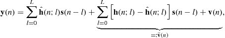
The DFE structure is shown in Figure 3.3 to equalize the delayed symbols ![]() , with the feed-forward (FF) and feed-back (FB) filters. Since each measurement
, with the feed-forward (FF) and feed-back (FB) filters. Since each measurement ![]() contains inter-symbol-interference (ISI) caused by prior symbols, DFE is designed to reduce ISI and to recover
contains inter-symbol-interference (ISI) caused by prior symbols, DFE is designed to reduce ISI and to recover ![]() using FIR filters. The FF filter takes current and prior measurements
using FIR filters. The FF filter takes current and prior measurements ![]() as its input to get information correlated with ISI and to remove its effect.
as its input to get information correlated with ISI and to remove its effect.
Stack the inputs of the FF filter with ![]() taps at time n into a “tall” vector
taps at time n into a “tall” vector
![]()
where ![]() is N -column vector and also define
is N -column vector and also define ![]() likewise. Then, the received signal is given as
likewise. Then, the received signal is given as
![]() (3.53)
(3.53)

where ![]() is
is ![]() matrix channel response at time n to a unit input at time
matrix channel response at time n to a unit input at time ![]() and
and ![]() is K-column vector. As shown in Figure 3.3, the input to the FB filter comes from the decision output, denoted by
is K-column vector. As shown in Figure 3.3, the input to the FB filter comes from the decision output, denoted by ![]() . The FB filter uses prior symbol decisions to cancel the trailing ISI by mapping the estimate
. The FB filter uses prior symbol decisions to cancel the trailing ISI by mapping the estimate ![]() to the closest point in the symbol constellation. We define the input vector of FB filter with
to the closest point in the symbol constellation. We define the input vector of FB filter with ![]() taps as
taps as
![]()
The estimate of the information symbol, ![]() is obtained by combining the outputs of FF and FB filters and can be written at time n with delay d as
is obtained by combining the outputs of FF and FB filters and can be written at time n with delay d as
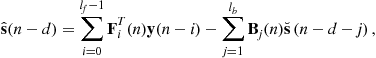 (3.54)
where ![]() s (that are
s (that are ![]() matrices) and
matrices) and ![]() s (that are
s (that are ![]() matrices) are the taps of FF and FB time-varying filters at time n, and
matrices) are the taps of FF and FB time-varying filters at time n, and ![]() is the hard decision of
is the hard decision of ![]() . The estimate
. The estimate ![]() is also fed into the quantizer to obtain the symbol decision
is also fed into the quantizer to obtain the symbol decision ![]() . Let
. Let ![]() and
and ![]() denote the vectors of time-varying taps of FF and FB filters,
denote the vectors of time-varying taps of FF and FB filters,
then the error signal is given by
![]() (3.55)
(3.55)
Assuming the decisions ![]() are correct and equal to
are correct and equal to ![]() , we can solve a nonlinear optimization problem which minimizes the variance of the error signal in (3.55),
, we can solve a nonlinear optimization problem which minimizes the variance of the error signal in (3.55),
![]() (3.56)
(3.56)
Solve a standard linear least-mean-squares estimation problem over ![]() with
with ![]() fixed and then we have a constrained optimization problem; note that the leading entry of
fixed and then we have a constrained optimization problem; note that the leading entry of ![]() is the identity matrix. Therefore, the FF and the FB time-varying filters of the MMSE-DFE are given by [69]
is the identity matrix. Therefore, the FF and the FB time-varying filters of the MMSE-DFE are given by [69]
![]() (3.57)
(3.57)
![]() (3.58)
(3.58)
where
By the assumption that ![]() are independent and identically distributed (i.i.d.) with variance
are independent and identically distributed (i.i.d.) with variance ![]() , and based on (3.53), we have
, and based on (3.53), we have
where
![]()
Using (3.57) and (3.58) in (3.54), we have the symbol estimate ![]() .
.
2.03.4.3 Maximum likelihood sequence detection
Maximum Likelihood Sequence Detector (MLSD) estimates the information sequence to maximize the joint probability of the received sequence conditioned on the information sequence. It is sequence estimator compared to the linear equalizers and DFE which are symbol-by-symbol detectors. For a scalar system a detailed discussion may be found in [1]; for MIMO channels see [71, Section 7.8]. The optimal equalization methods for minimizing sequence error rate or the bit error rate (BER) are based on MAP (maximum a posteriori) estimation, which turns into maximum likelihood (ML) estimation when the transmitted symbols are equally likely. For instance, see Viterbi algorithm (VA) [1,72,73] for ML sequence estimation and BCJR algorithm [74] for MAP sequence estimation. The MAP/ML-based solutions often suffer from high computational load for channels with long memory or large constellation sizes. For model (3.9), the ML estimate of the channel input sequence ![]() based on a sequence of channel output
based on a sequence of channel output ![]() and given knowledge of the channel, can be obtained by maximizing the likelihood function, or equivalently, by minimizing
and given knowledge of the channel, can be obtained by maximizing the likelihood function, or equivalently, by minimizing
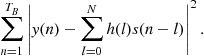 (3.59)
If the symbol alphabet size is M, then the Viterbi algorithm can be implemented by denoting ![]() states as all possible L-tuples of
states as all possible L-tuples of ![]() . The trellis is determined by the symbol alphabet
. The trellis is determined by the symbol alphabet ![]() while the metrics of the Viterbi algorithm depend upon the channel.
while the metrics of the Viterbi algorithm depend upon the channel.
2.03.4.4 Turbo equalization
In turbo equalization one exploits the information obtained from a channel decoder to improve equalization. A practical digital communication system has a forward error correction (FEC) channel encoder at the transmitter which adds redundancies to the information symbols before transmitting the encoded sequence over the channel. At the receiver, compensation for channel distortions is the task of equalizers while subsequent recovery of the data symbols from the equalized (and quantized) symbols making use of the FEC encoding is the task for the channel decoder. Typically these two tasks are considered separately (to reduce computational complexity) with limited interaction between the two [75]. An optimal joint processing of the equalization and decoding steps is usually impossible due to complexity considerations. A number of iterative receiver algorithms repeat the equalization and decoding tasks on the same set of received data, where feedback information from the decoder is incorporated into the equalization process. This method, called turbo equalization, was originally developed for concatenated convolutional codes (turbo code [76]) and is now adapted to various communication problems.
Communicating soft information probability distribution between the equalizer and the decoder, instead of hard information (symbol estimates only), improves the BER performance but usually requires more complex decoding algorithms. State-of-the-art systems for a variety of communication channels employ convolutional codes and ML equalizers together with an interleaver after the encoder and a deinterleaver before the decoder [75]. Interleaving shuffles symbols within a given time frame or block of data and thus decorrelates error events introduced by the equalizer between neighboring symbols. The MAP/ML-based solutions often suffer from high computational load for channels with long memory or large constellation sizes (expensive equalizer) or convolutional codes with long memory (expensive decoder). This situation is exacerbated by the need to perform equalization and decoding several times for each block of data. A major research issue is thus the complexity reduction of such iterative algorithms.
2.03.4.4.1 Principle of turbo equalization
Consider a simple transmitter where a sequence of data ![]() is encoded to the code symbols
is encoded to the code symbols ![]() with a code rate
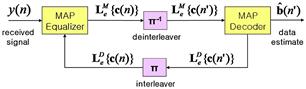
with a code rate ![]() , which is interleaved in a block and then mapped into binary phase shift keying (BPSK) symbols. Figure 3.4 depicts the receiver structure for turbo equalization [77], where both the soft-input soft-output (
, which is interleaved in a block and then mapped into binary phase shift keying (BPSK) symbols. Figure 3.4 depicts the receiver structure for turbo equalization [77], where both the soft-input soft-output (![]() : we use subscript f to distinguish between single-input single-output abbreviated as SISO and soft-input soft-output abbreviated as
: we use subscript f to distinguish between single-input single-output abbreviated as SISO and soft-input soft-output abbreviated as ![]() ) equalizer and
) equalizer and ![]() decoder are of the MAP type. The extrinsic log-likelihood ratios (LLRs),
decoder are of the MAP type. The extrinsic log-likelihood ratios (LLRs), ![]() are transferred iteratively between the equalizer and decoder. [The subscript “e” for representing “extrinsic,” the superscript “E” and “D” for output of “Equalizer” and “Decoder” respectively]. The MAP equalizer computes the a posteriori probabilities (APPs) given
are transferred iteratively between the equalizer and decoder. [The subscript “e” for representing “extrinsic,” the superscript “E” and “D” for output of “Equalizer” and “Decoder” respectively]. The MAP equalizer computes the a posteriori probabilities (APPs) given ![]() received symbols,
received symbols, ![]() and generates the extrinsic LLR as (a posteriori LLR – a priori LLR)
and generates the extrinsic LLR as (a posteriori LLR – a priori LLR)
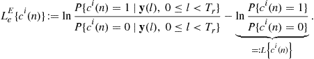 (3.60)
The a priori LLR of the MAP equalizer, ![]() is provided by the interleaved output of the MAP decoder at the previous iteration but
is provided by the interleaved output of the MAP decoder at the previous iteration but ![]() for the first iteration. The extrinsic LLRs
for the first iteration. The extrinsic LLRs ![]() produced by the MAP demodulator is sent to the MAP decoder as the a priori LLRs for channel decoding. Based on the a priori LLRs and the channel code constraints, the MAP decoder computes the APPs
produced by the MAP demodulator is sent to the MAP decoder as the a priori LLRs for channel decoding. Based on the a priori LLRs and the channel code constraints, the MAP decoder computes the APPs ![]() and generates the extrinsic LLR as
and generates the extrinsic LLR as
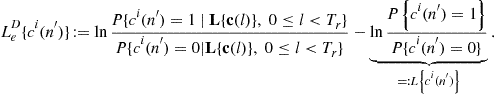 (3.61)
The extrinsic output of the MAP decoder is fed back to the MAP equalizer iteratively. Note that (3.60) and (3.61) are valid only if the a posteriori outputs are independent of the a priori inputs for the equalizer and the decoder. Assuming ideal interleaver between the equalizer and the decoder, we can apply the turbo principle and the correct ordering of the LLRs ![]() and
and ![]() , which are input to the MAP decoder and the MAP equalizer respectively. The MAP decoder also compute the a posteriori probabilities of the input data bit and then the data estimate
, which are input to the MAP decoder and the MAP equalizer respectively. The MAP decoder also compute the a posteriori probabilities of the input data bit and then the data estimate ![]() as
as
![]() (3.62)
(3.62)
By combining a MAP equalizer and a MAP decoder, and exchanging probabilistic information about data symbols iteratively, turbo equalization usually can achieve close-to-optimal performance but much lower complexity [77,78]. In [79], a turbo-equalization-like system using linear equalizers based on soft interference cancellation and linear minimum mean-square error (MMSE) filtering is proposed as part of a multiuser detector for CDMA. Based on this work, a variety of ![]() equalizers employing linear MMSE and decision feedback equalization (DFE) are proposed in [75,80,81].
equalizers employing linear MMSE and decision feedback equalization (DFE) are proposed in [75,80,81].
2.03.4.4.2 Turbo equalization for doubly-selective channels
For doubly-selective channels, an adaptive ![]() equalizer has been presented in [5], using extended Kalman filter (EKF) to incorporate channel estimation into the equalization process. This adaptive soft nonlinear Kalman equalizer takes the soft decisions of data symbols from the
equalizer has been presented in [5], using extended Kalman filter (EKF) to incorporate channel estimation into the equalization process. This adaptive soft nonlinear Kalman equalizer takes the soft decisions of data symbols from the ![]() decoder as its a priori information, and performs equalization process iteratively. With such an approach, the proposed scheme jointly optimizes the estimates of the channel and data symbols in each iteration. This avoids the common drawback in separate channel estimation and equalization/detection approach in that the correlation between channel estimate and data symbol decision is considered. The complexity of the method of [5] is comparable to that of the turbo equalizers using linear filters [82–84], and is usually much lower than that of the ML/MAP based joint channel estimation and data detection schemes.
decoder as its a priori information, and performs equalization process iteratively. With such an approach, the proposed scheme jointly optimizes the estimates of the channel and data symbols in each iteration. This avoids the common drawback in separate channel estimation and equalization/detection approach in that the correlation between channel estimate and data symbol decision is considered. The complexity of the method of [5] is comparable to that of the turbo equalizers using linear filters [82–84], and is usually much lower than that of the ML/MAP based joint channel estimation and data detection schemes.
Based on the turbo equalization approach proposed in [5] and CE-BEM, an adaptive turbo equalizer with nonlinear Kalman filtering has been proposed in [85]. It is discussed in more detail in later under adaptive channel estimation and equalization.
2.03.5 Precoding
Thus far we have discussed channel estimation and equalization at the receiver. The basic idea behind channel precoding is that if the channel state information (CSI) is known at the transmit side, one can move the “equalizer” to the transmitter thereby simplifying the equalizer at the receiver and/or minimizing noise enhancement at the receiver [1,86–88]. In the SISO case precoding helps in ISI mitigation. In the MIMO case the objective is both ISI cancellation and multiuser/multiantenna interference mitigation. The book [87] provides a recent comprehensive review of recent advances, and [89,90] are good review articles for SISO and MIMO channels, respectively.
2.03.5.1 Precoding for SISO channels
Precoding the information symbols at the transmitter with full knowledge of CSI to mitigate ISI was first proposed in [86,88]. Since then it has been generalized to a wide variety of scenarios [87,89,90]. In the original works of [86,88], real-valued M ary PAM (pulse amplitude modulation) signal set was considered which is what we do here. The information alphabet is taken from the set ![]() . Consider the channel given by (3.9). Unlike (3.9), the information symbol
. Consider the channel given by (3.9). Unlike (3.9), the information symbol ![]() is precoded to
is precoded to ![]() chosen from
chosen from ![]() as follows
as follows
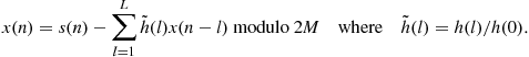 (3.63)
The transmitter transmits the precoded sequence ![]() instead of
instead of ![]() over the channel represented by (3.9). At the receiver one has
over the channel represented by (3.9). At the receiver one has ![]() . By (3.63) there exists a unique integer
. By (3.63) there exists a unique integer ![]() such that
such that
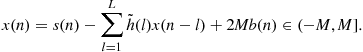 (3.64)
Using z-transform of the sequences in (3.64) we have
![]() (3.65)
(3.65)
Therefore at the receiver we have the ![]() -transform of the received sequence
-transform of the received sequence ![]() as
as
![]() (3.66)
(3.66)
2.03.5.2 Precoding for MIMO channels
This is a very active area of current research [87,90] and our overview will be quite brief. The basic idea here is to map a block of information symbols ![]() into a larger block of data
into a larger block of data ![]() via some linear transformation (precoding)
via some linear transformation (precoding) ![]() , and the precoded symbol block
, and the precoded symbol block ![]() is then modulated and transmitted over the channel. At the receiver one designs a decoder
is then modulated and transmitted over the channel. At the receiver one designs a decoder ![]() to operate on the noisy received signal block
to operate on the noisy received signal block ![]() (
(![]() represents the channel effect) to yield the symbol block estimate
represents the channel effect) to yield the symbol block estimate ![]() . The structure of
. The structure of ![]() , the redundancy added per block and the design criteria for the choice of precoder-decoder pair
, the redundancy added per block and the design criteria for the choice of precoder-decoder pair ![]() and
and ![]() together with the underlying channel matrix
together with the underlying channel matrix ![]() dictate the resulting performance of the system.
dictate the resulting performance of the system.
Consider (3.49) with K users (transmit antennas), N receive antennas and input of precoded symbols ![]() instead of information symbols
instead of information symbols ![]() . Following [91], for some integer
. Following [91], for some integer ![]() , let
, let ![]() and define the blocks
and define the blocks
![]() (3.67)
(3.67)
![]() (3.68)
(3.68)
where ![]() is
is ![]() and
and ![]() is
is ![]() . In (3.68) the first L vectors have been deleted to cancel interblock interference (IBI); an alternative is to zero-pad the tail of every block
. In (3.68) the first L vectors have been deleted to cancel interblock interference (IBI); an alternative is to zero-pad the tail of every block ![]() [91]. From (3.49), (3.67), and (3.68), one can deduce
[91]. From (3.49), (3.67), and (3.68), one can deduce
![]() (3.69)
(3.69)
where ![]() is an
is an ![]() block-banded matrix and it becomes a block Toeplitz matrix for time-invariant channels. A block of
block-banded matrix and it becomes a block Toeplitz matrix for time-invariant channels. A block of ![]() information symbols
information symbols ![]() is precoded as
is precoded as
![]() (3.70)
(3.70)
In [91] under additive white Gaussian noise, various designs of precoder-decoder pairs ![]() are considered. Let
are considered. Let
![]() (3.71)
(3.71)
For given ![]() and
and ![]() , decoder
, decoder ![]() is chosen to minimize
is chosen to minimize ![]() . Then under a transmit power or similar constraint,
. Then under a transmit power or similar constraint, ![]() is chosen to minimize a function of
is chosen to minimize a function of ![]() .
.
The joint linear precoder/decoder design is in general a complicated non-convex problem [87]. The linear precoder/decoder optimization decouples the MIMO channel into parallel subchannels if the criterion is the minimization of the weighted sum of MSEs of all subchannels. Note also that MSE is not the only criterion for precoder design; other criteria include maximization of SNR, maximization of information rate, and minimization of bit error probability [87].
2.03.5.3 Precoding with partial or no CSI at transmitter
When the channel is time-varying, the assumption of knowledge of CSI at the transmitter is not entirely justified. Then an appropriate approach is to design precoder/decoder on the basis of the statistical knowledge of the CSI or resort to blind methods. For precoder designs using the first- and second-order statistics of the channels at the transmitter, see [92] and references therein. Precoding can also facilitate blind channel estimation and equalization in the absence of any training; see [93,94] and references therein.
A fairly comprehensive review of some of these issues and techniques may be found in [87,90].
2.03.6 Tracking
2.03.6.1 Adaptive channel estimation for slowly varying channels
When the channel characteristics vary slowly with time, recursive implementations of the “traditional” (linear or DFE) equalizers aided with initial transmission of a training sequence work well [1, Chapter 11]. The equalization parameters are often updated through the MMSE criterion. This requires that a known channel input sequence be transmitted initially. Adaptive channel equalizers begin adaptation with the assistance of a known training sequence transmitted during the initial training stage by the transmitter. Since the input signal is available, adaptive algorithms can be used to adjust the equalizer parameters by minimizing the MSE between the equalizer output and the known channel input with an equalization delay ![]() . After training, equalizer parameters should be sufficiently close to the desired settings such that much of the ISI is removed. As the channel input can now be correctly recovered from the equalizer output through a decision device (hard quantizer), the second (operational) stage can begin. In the operational stage, the receivers typically switch to decision-directed mode where the equalized signal is sent to a symbol detector and the detected symbols are used as a (pseudo-)training sequence to update equalizer coefficients. Baud-rate linear transversal equalizers, FSE and DFE all can be updated in this way. During either stage, the equalizer parameters can be determined using the well-known recursive least-squares (RLS) or least mean square (LMS) algorithms [1,70].
. After training, equalizer parameters should be sufficiently close to the desired settings such that much of the ISI is removed. As the channel input can now be correctly recovered from the equalizer output through a decision device (hard quantizer), the second (operational) stage can begin. In the operational stage, the receivers typically switch to decision-directed mode where the equalized signal is sent to a symbol detector and the detected symbols are used as a (pseudo-)training sequence to update equalizer coefficients. Baud-rate linear transversal equalizers, FSE and DFE all can be updated in this way. During either stage, the equalizer parameters can be determined using the well-known recursive least-squares (RLS) or least mean square (LMS) algorithms [1,70].
In the absence of training, blind equalizers may be employed; they tend to be much slower in convergence and tracking.
2.03.6.2 Block-adaptive channel estimation using CE-BEM
Here we summarize the time-multiplexed training approach of [11]. In [11] each transmitted block of symbols ![]() is segmented into
is segmented into ![]() subblocks of time-multiplexed training and information symbols. Each subblock is of equal length
subblocks of time-multiplexed training and information symbols. Each subblock is of equal length ![]() symbols with
symbols with ![]() information symbols and
information symbols and ![]() training symbols (
training symbols (![]() ). If
). If ![]() denotes a column-vector composed of
denotes a column-vector composed of ![]() , then
, then ![]() is arranged as
is arranged as
![]() (3.72)
(3.72)
where ![]() is a column of
is a column of ![]() information symbols and
information symbols and ![]() is a column of
is a column of ![]() training symbols. We clearly have
training symbols. We clearly have ![]() . Given (3.8) and CE-BEM (3.17), Ma et al. [11] has shown that (3.72) is an optimum structure for
. Given (3.8) and CE-BEM (3.17), Ma et al. [11] has shown that (3.72) is an optimum structure for ![]() with
with ![]() and
and
![]() (3.73)
(3.73)
Thus, given a transmission block of size ![]() symbols have to be devoted to training and the remaining
symbols have to be devoted to training and the remaining ![]() are available for information symbols.
are available for information symbols.
Let ![]() (
(![]() ) denote the location of (nonzero)
) denote the location of (nonzero) ![]() ’s in the optimum
’s in the optimum ![]() ’s in the P subblocks. Then by design, received signal (assuming timing synchronization)
’s in the P subblocks. Then by design, received signal (assuming timing synchronization)
![]() (3.74)
(3.74)
for ![]() . Using (3.17) in these
. Using (3.17) in these ![]() s, one can uniquely obtain
s, one can uniquely obtain ![]() s via a least-squares approach. The channel estimates are given by the CE-BEM (3.17) using the estimated BEM coefficients.
s via a least-squares approach. The channel estimates are given by the CE-BEM (3.17) using the estimated BEM coefficients.
2.03.6.3 Adaptive channel estimation via subblock tracking
Suppose that we collect the received signal over a time interval of ![]() symbols. We wish to estimate the time-variant channel using a channel model and time-multiplexed training (such as that discussed in Section 2.03.6.2 and [11]), and subsequently using the estimated channel, estimate the information symbols. For CE-BEM, if we choose
symbols. We wish to estimate the time-variant channel using a channel model and time-multiplexed training (such as that discussed in Section 2.03.6.2 and [11]), and subsequently using the estimated channel, estimate the information symbols. For CE-BEM, if we choose ![]() as the block size, then in general Q value will be very high requiring estimation of a large number of parameters, thereby degrading the channel estimation performance. If we divide
as the block size, then in general Q value will be very high requiring estimation of a large number of parameters, thereby degrading the channel estimation performance. If we divide ![]() into blocks of size
into blocks of size ![]() , and then fit CE-BEM block by block, we need smaller Q; however, estimation of
, and then fit CE-BEM block by block, we need smaller Q; however, estimation of ![]() ’s is now based on a shorter observation size of
’s is now based on a shorter observation size of ![]() symbols which might also degrade channel estimation performance. Thus one has to strike a balance between estimation variance and block size. Such considerations do not apply to the AR channel model fitting. [95] proposes a novel subblock tracking approach to CE-BEM channel estimation where one updates estimates of
symbols which might also degrade channel estimation performance. Thus one has to strike a balance between estimation variance and block size. Such considerations do not apply to the AR channel model fitting. [95] proposes a novel subblock tracking approach to CE-BEM channel estimation where one updates estimates of ![]() s every subblock based on all of the past training symbols (see Figure 3.5).
s every subblock based on all of the past training symbols (see Figure 3.5).
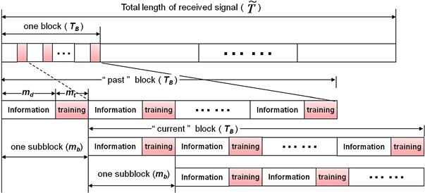
Figure 3.5 Subblock-wise channel estimation: overlapping blocks and subblocks, where one block comprises several subblocks and each subblock has an information session followed by a training session.
By exploiting the invariance of the coefficients of CE-BEM over each block, hence, each of the ![]() subblocks per block of length
subblocks per block of length ![]() symbols, one seeks subblock-wise tracking of the BEM coefficients of the doubly-selective channel. Consider two overlapping blocks that differ by just one subblock: blocks with
symbols, one seeks subblock-wise tracking of the BEM coefficients of the doubly-selective channel. Consider two overlapping blocks that differ by just one subblock: blocks with ![]() where
where ![]() for the “past” block and
for the “past” block and ![]() for the “current” block. If the two blocks overlap so significantly, one would expect the BEM coefficients to vary only a little from the past block to the current overlapping block. Therefore, rather than estimate
for the “current” block. If the two blocks overlap so significantly, one would expect the BEM coefficients to vary only a little from the past block to the current overlapping block. Therefore, rather than estimate ![]() s anew with every non-overlapping block as in Section 2.03.6.2 and [11], one can track the BEM coefficients subblock by subblock using a first-order AR model for their variations. Stack the channel coefficients in (3.17) into vectors
s anew with every non-overlapping block as in Section 2.03.6.2 and [11], one can track the BEM coefficients subblock by subblock using a first-order AR model for their variations. Stack the channel coefficients in (3.17) into vectors
![]() (3.75)
(3.75)
![]() (3.76)
(3.76)
of size Q and ![]() respectively. The coefficient vector in (3.76) for the pth subblock (
respectively. The coefficient vector in (3.76) for the pth subblock (![]() ) will be denoted by
) will be denoted by ![]() . We assume that the BEM coefficients over each subblock are Markovian: a simplified model is given by the first-order AR process, i.e.,
. We assume that the BEM coefficients over each subblock are Markovian: a simplified model is given by the first-order AR process, i.e.,
![]() (3.77)
(3.77)
where ![]() is the AR coefficient, and the driving noise vector
is the AR coefficient, and the driving noise vector ![]() is zero-mean complex Gaussian with variance
is zero-mean complex Gaussian with variance ![]() and statistically independent of
and statistically independent of ![]() . If the channel is stationary and coefficients
. If the channel is stationary and coefficients ![]() s are independent (as assumed in [11]), then it follows from (3.77) that
s are independent (as assumed in [11]), then it follows from (3.77) that ![]() with
with ![]() . Since the coefficients evolve slowly, we have
. Since the coefficients evolve slowly, we have ![]() (but
(but ![]() for tracking). Under this formulation we do not have a “strict” definition of the block size
for tracking). Under this formulation we do not have a “strict” definition of the block size ![]() because, although we still use (3.17) for any n, we allow
because, although we still use (3.17) for any n, we allow ![]() s to change subblock by subblock based on the training symbols.
s to change subblock by subblock based on the training symbols.
Define ![]() . If at time n the pth subblock is being received, by (3.6), (3.17–3.19) and (3.75–3.76), the received signal can be written as
. If at time n the pth subblock is being received, by (3.6), (3.17–3.19) and (3.75–3.76), the received signal can be written as
![]() (3.78)
(3.78)
where ![]() . Treating (3.77) and (3.78) as the state and the measurement equations respectively, Kalman filtering can be applied to track the coefficient vector
. Treating (3.77) and (3.78) as the state and the measurement equations respectively, Kalman filtering can be applied to track the coefficient vector ![]() for each subblock; further details are in [95]. Alternatively, one can devise RLS-based approaches for subblock-based tracking one does not need any prior models for BEM coefficients; further details are in [95].
for each subblock; further details are in [95]. Alternatively, one can devise RLS-based approaches for subblock-based tracking one does not need any prior models for BEM coefficients; further details are in [95].
2.03.6.4 Symbol-adaptive joint channel estimation and data detection
Representative approaches in this category are [4,5] and references therein. A Gauss-Markov model for channel variations (typically an autoregressive model) is coupled with a state-space model for received data to form an augmented state-space model with nonlinear measurement equation. This results in a nonlinear state estimation problem. In [4] a finite-length minimum mean-square error (MMSE) DFE is used during non-data-aided periods to generate hard decisions. Reference [5] presents a low complexity turbo equalization receiver for coded signals where a nonlinear Kalman filtering based adaptive equalizer (using Extended Kalman Filter (EKF)) is coupled with a soft-in soft-out decoder. These approaches work well so long as the channel does not fade too fast.
2.03.6.4.1 Turbo equalization using EKF and CE-BEM
Now we describe an extension of [5] as reported in [85] where a CE-BEM-based subblock tracking model (with one sample long subblock) is used. Kin and Tuguait [85] considers two overlapping blocks (each of ![]() symbols) that differ by just one symbol: the “past” block beginning at time
symbols) that differ by just one symbol: the “past” block beginning at time ![]() and the “present” block beginning at time
and the “present” block beginning at time ![]() . Since the two blocks overlap so significantly, one would expect the BEM coefficients to vary only “a little” from the past block to the present overlapping one. One can track the BEM coefficients (rather than the channel tap gains) symbol-by-symbol using a first-order AR model for their variations. Kin and Tuguait [85] use (3.17) for all times n, not just the particular block of size
. Since the two blocks overlap so significantly, one would expect the BEM coefficients to vary only “a little” from the past block to the present overlapping one. One can track the BEM coefficients (rather than the channel tap gains) symbol-by-symbol using a first-order AR model for their variations. Kin and Tuguait [85] use (3.17) for all times n, not just the particular block of size ![]() symbols, by allowing the coefficients
symbols, by allowing the coefficients ![]() s to change with time. Note that model (3.17) is periodic with period
s to change with time. Note that model (3.17) is periodic with period ![]() whereas the channel is by no means periodic. So long as the effective “memory” of the Kalman filter used later is less than the model period
whereas the channel is by no means periodic. So long as the effective “memory” of the Kalman filter used later is less than the model period ![]() , there are no deleterious effects due to the use of (3.17) for all time.
, there are no deleterious effects due to the use of (3.17) for all time.
Bit-Interleaved Coded Modulation (BICM). We consider a BICM transmitter (as in [96]) for a doubly-selective fading channel as shown in Figure 3.6. A sequence of independent data vector ![]() are fed into a convolutional encoder with a code rate
are fed into a convolutional encoder with a code rate ![]() . The coded output
. The coded output ![]() is passed through a bit-wise random interleaver
is passed through a bit-wise random interleaver ![]() , generating the interleaved coded bit sequence
, generating the interleaved coded bit sequence ![]() . The binary coded bits are then mapped to a signal sequence
. The binary coded bits are then mapped to a signal sequence ![]() over a 2-dimensional signal constellation
over a 2-dimensional signal constellation ![]() of cardinality
of cardinality ![]() by a
by a ![]() -ary modulator with an one-to-one binary map
-ary modulator with an one-to-one binary map ![]() . In this section, we only consider the case of phase-shift keying (PSK) or quadrature amplitude modulation (QAM) with the average energy of the constellation
. In this section, we only consider the case of phase-shift keying (PSK) or quadrature amplitude modulation (QAM) with the average energy of the constellation ![]() to be unity. That is, the signal
to be unity. That is, the signal ![]() drawn from
drawn from ![]() has mean
has mean ![]() and variance
and variance ![]() . After modulation, we periodically insert short training sequences into the data symbol sequence. The training symbols
. After modulation, we periodically insert short training sequences into the data symbol sequence. The training symbols ![]() , which are known to the receiver, are randomly drawn from the signal constellation
, which are known to the receiver, are randomly drawn from the signal constellation ![]() with equal probabilities. The symbol
with equal probabilities. The symbol ![]() will be used to denote the symbol sequence after training
will be used to denote the symbol sequence after training ![]() insertion into data symbol sequence
insertion into data symbol sequence ![]() .
.
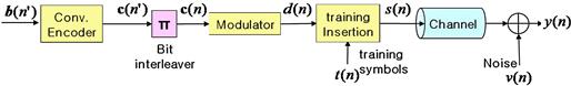
Receiver structure. A turbo equalization structure, as depicted in Figure 3.7, is employed in the receiver, as in [5] except that [5] uses symbol-wise AR models. The adaptive ![]() equalizer is embedded into the iterative decoding (ID) process of the BICM transmission system (BICM-ID) [96]. In each decoding iteration, the equalizer takes the training symbols and the soft decision information about data symbols supplied by the
equalizer is embedded into the iterative decoding (ID) process of the BICM transmission system (BICM-ID) [96]. In each decoding iteration, the equalizer takes the training symbols and the soft decision information about data symbols supplied by the ![]() decoder from the previous iteration as its a priori information to perform joint adaptive channel estimation and equalization. The equalizer produces the soft-valued extrinsic estimate of the data symbols, which are independent of their a priori information. The output of the equalizer is an updated sequence of soft estimates
decoder from the previous iteration as its a priori information to perform joint adaptive channel estimation and equalization. The equalizer produces the soft-valued extrinsic estimate of the data symbols, which are independent of their a priori information. The output of the equalizer is an updated sequence of soft estimates ![]() and its error variance
and its error variance ![]() . Using the adaptive
. Using the adaptive ![]() equalizer described later, we have extrinsic information for the data symbols
equalizer described later, we have extrinsic information for the data symbols ![]() . The training symbols are removed at the
. The training symbols are removed at the ![]() equalizer output and the iterative process that follows is only for data symbols. The
equalizer output and the iterative process that follows is only for data symbols. The ![]() equalizer based on the CE-BEM is described later. The
equalizer based on the CE-BEM is described later. The ![]() demodulator follows [96] whereas the
demodulator follows [96] whereas the ![]() decoder follows the MAP decoding algorithm (“BCJR”) [99] Section 6.2.
decoder follows the MAP decoding algorithm (“BCJR”) [99] Section 6.2.

Figure 3.7 Turbo equalization receiver. Following [5,97,98] and contrary to the original turbo principle, a posteriori LLR ![]() instead of the extrinsic LLR
instead of the extrinsic LLR ![]() can be input to the LLR-to-symbol block. Inclusion of
can be input to the LLR-to-symbol block. Inclusion of ![]() to create a posteriori LLR is shown via dashed line. For our proposed approach we follow [5,97,98].
to create a posteriori LLR is shown via dashed line. For our proposed approach we follow [5,97,98].
Adaptive![]() nonlinear Kalman equalizer. Using a symbol-wise AR-model for channel variations, an adaptive
nonlinear Kalman equalizer. Using a symbol-wise AR-model for channel variations, an adaptive ![]() equalizer using fixed-lag EKF was presented in [5] for joint channel estimation and equalization where their correlation was (implicitly) considered. The CE-BEM model-based
equalizer using fixed-lag EKF was presented in [5] for joint channel estimation and equalization where their correlation was (implicitly) considered. The CE-BEM model-based ![]() nonlinear Kalman equalizer for turbo equalization follows a similar approach. We will perform equalization with a delay
nonlinear Kalman equalizer for turbo equalization follows a similar approach. We will perform equalization with a delay ![]() . Define a parameter
. Define a parameter
![]() (3.79)
(3.79)
and the data vector
![]() (3.80)
(3.80)
In order to apply (extended) Kalman filtering to joint channel estimation and equalization, we stack ![]() (which is given by (3.77) after replacing p therein with n to reflect the fact our subblock size now is one sample) and data vector
(which is given by (3.77) after replacing p therein with n to reflect the fact our subblock size now is one sample) and data vector ![]() together into a
together into a ![]() state vector
state vector ![]() at time n as
at time n as
![]() (3.81)
(3.81)
As in [5] (and others), we consider the symbol sequence ![]() as a stochastic process so as to utilize the soft decisions on the data symbols generated in the iterative decoding process as its a priori information. We can express
as a stochastic process so as to utilize the soft decisions on the data symbols generated in the iterative decoding process as its a priori information. We can express ![]() as
as ![]() where
where ![]() and
and ![]() is approximated as a zero-mean uncorrelated sequence such that
is approximated as a zero-mean uncorrelated sequence such that ![]() , assuming an ideal interleaver. Note that
, assuming an ideal interleaver. Note that ![]() and
and ![]() are provided via the a priori information. We have
are provided via the a priori information. We have ![]() and
and ![]() for a data symbol
for a data symbol ![]() (where
(where ![]() and
and ![]() are obtained from the extrinsic LLRs of the
are obtained from the extrinsic LLRs of the ![]() decoder), while
decoder), while ![]() and
and ![]() for a training symbol
for a training symbol ![]() . Using
. Using ![]() , the state equation turns out to be
, the state equation turns out to be
![]() (3.82)
(3.82)
where
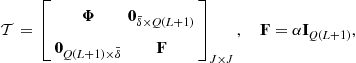 (3.83)
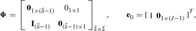 (3.84)
the vector
![]() (3.85)
(3.85)
is zero-mean uncorrelated process noise where ![]() is given in (3.77) and
is given in (3.77) and
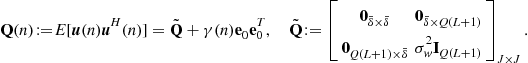 (3.86)
The channel output ![]() in (3.6) can be rewritten by CE-BEM given in (3.17) as
in (3.6) can be rewritten by CE-BEM given in (3.17) as
![]() (3.87)
(3.87)
where ![]() and
and ![]() . Using the state vector that comprises the information symbols and channel coefficients, the measurement equation can be given as
. Using the state vector that comprises the information symbols and channel coefficients, the measurement equation can be given as
![]() (3.88)
(3.88)
where
 (3.89)
With (3.82) and (3.88) as the state and measurement equations, respectively, nonlinear Kalman filtering via EKF is applied to track ![]() for joint channel estimation and equalization.
for joint channel estimation and equalization.
Structure of adaptive soft-input soft-output equalizer. The fixed-lag EKF takes soft inputs and generates a delayed a posteriori estimate for ![]() . In order to generate extrinsic estimate independent of the a priori information
. In order to generate extrinsic estimate independent of the a priori information ![]() , a “comb” structure in conjunction with the EKF in Figure 3.8 is used for the
, a “comb” structure in conjunction with the EKF in Figure 3.8 is used for the ![]() equalization, just as in [5]. At each time n, the vertical branch composed of
equalization, just as in [5]. At each time n, the vertical branch composed of ![]() EKFs produce the extrinsic estimate
EKFs produce the extrinsic estimate ![]() , while the horizontal branch keeps updating the a posteriori estimate
, while the horizontal branch keeps updating the a posteriori estimate ![]() and its error covariance
and its error covariance ![]() ; here
; here ![]() denotes the estimate of
denotes the estimate of ![]() given the observations
given the observations ![]() , and
, and ![]() denotes the error covariance matrix of
denotes the error covariance matrix of ![]() . The first vertical EKF has an input
. The first vertical EKF has an input ![]() in place of
in place of ![]() to exclude the effect of the a priori information. Let
to exclude the effect of the a priori information. Let ![]() and
and ![]() denote the state estimate and its error covariance matrix, respectively, generated by the
denote the state estimate and its error covariance matrix, respectively, generated by the ![]() th vertical filtering branch. Then the extrinsic estimate
th vertical filtering branch. Then the extrinsic estimate ![]() of
of ![]() and its error variance
and its error variance ![]() are given by
are given by
![]() (3.90)
(3.90)
![]() (3.91)
(3.91)
Note that the extrinsic outputs ![]() and
and ![]() are computed for data symbol
are computed for data symbol ![]() , not for training symbol
, not for training symbol ![]() , and then used in the later parts of the turbo-equalization receiver (see Figure 3.7). Further details regarding generation of extrinsic estimates can be found in [5].
, and then used in the later parts of the turbo-equalization receiver (see Figure 3.7). Further details regarding generation of extrinsic estimates can be found in [5].

Figure 3.8 Structure of the adaptive ![]() equalizer proposed in [5].
equalizer proposed in [5].
Simulation examples. A random time- and frequency-selective Rayleigh fading channel is considered. We assume ![]() is zero-mean, complex Gaussian, and white with autocorrelation
is zero-mean, complex Gaussian, and white with autocorrelation ![]() . We take
. We take ![]() (3 taps) and
(3 taps) and ![]() . For different ls,
. For different ls, ![]() s are mutually independent and satisfy Jakes’ model. To this end, we simulate each single tap following [100] (with a correction in the Appendix of [13]). We consider a normalized Doppler spread
s are mutually independent and satisfy Jakes’ model. To this end, we simulate each single tap following [100] (with a correction in the Appendix of [13]). We consider a normalized Doppler spread ![]() from 0.001 to 0.01. The additive noise is zero-mean complex white Gaussian. The (receiver) SNR refers to the average energy per symbol over one-sided noise spectral density. In the simulations, we use a four-state convolutional code of rate
from 0.001 to 0.01. The additive noise is zero-mean complex white Gaussian. The (receiver) SNR refers to the average energy per symbol over one-sided noise spectral density. In the simulations, we use a four-state convolutional code of rate ![]() with octal generators
with octal generators ![]() . The information block size is set to 3000 bits (
. The information block size is set to 3000 bits (![]() ) leading to a coded block size of 6000 bits, and the interleaver size is equal to the coded block size. In the modulator, the QPSK constellation with Gray mapping is used, which gives
) leading to a coded block size of 6000 bits, and the interleaver size is equal to the coded block size. In the modulator, the QPSK constellation with Gray mapping is used, which gives ![]() and a block size of 3000 symbols. After modulation, training symbol sequences of length
and a block size of 3000 symbols. After modulation, training symbol sequences of length ![]() are inserted in front of every
are inserted in front of every ![]() data symbols, leading to a sequence of length
data symbols, leading to a sequence of length ![]() when
when ![]() and
and ![]() (20% training overhead).
(20% training overhead).
We compared the following schemes:
• The approach of [83] that uses the linear MMSE equalizer (e.g., [80]) coupled with modified RLS channel estimation, where we set the linear filter length ![]() (6 pre-cursor taps and 3 post-cursor taps are used). This scheme is denoted by “TE-LE.”
(6 pre-cursor taps and 3 post-cursor taps are used). This scheme is denoted by “TE-LE.”
• The AR(p) model-based scheme in [5]. The AR(p) model is fitted using [3] to Jakes’ spectrum with ![]() (the maximum anticipated normalized Doppler spread), denoted by “TE-AR5” for AR(5) model and “TE-AR9” for AR(9) model.
(the maximum anticipated normalized Doppler spread), denoted by “TE-AR5” for AR(5) model and “TE-AR9” for AR(9) model.
• The proposed BEM-based turbo equalization schemes, where we consider BEM period ![]() and 400 respectively, so that
and 400 respectively, so that ![]() and 9 , respectively, by (3.19). For the channel BEM coefficients, we take the AR-coefficient in (3.17) as
and 9 , respectively, by (3.19). For the channel BEM coefficients, we take the AR-coefficient in (3.17) as ![]() for
for ![]() and
and ![]() for
for ![]() . This scheme is denoted by “TE-BEM(200)” for
. This scheme is denoted by “TE-BEM(200)” for ![]() and “TE-BEM(400)” for
and “TE-BEM(400)” for ![]() .
.
• The turbo equalizer based on the fixed-lag Kalman filter with perfect knowledge of the true channel, denoted by “TrueCH.”
• The turbo equalizer based on the optimum trellis-based MAP (BJCR) method [101] with perfect knowledge of the true channel, denoted by “Opt-MAP-TrueCH.”
We evaluate the performances of various schemes by considering their normalized channel mean square error (NCMSE) and their bit error rates (BER). The NCMSE is defined as

where ![]() is the true channel and
is the true channel and ![]() is the estimated channel at the ith Monte Carlo run, among total
is the estimated channel at the ith Monte Carlo run, among total ![]() runs. The BERs are evaluated by employing the equalization delay
runs. The BERs are evaluated by employing the equalization delay ![]() , using the decoded information symbol sequences at the turbo-equalization receiver. All the simulation results are based on 1000 runs.
, using the decoded information symbol sequences at the turbo-equalization receiver. All the simulation results are based on 1000 runs.
In Figures 3.9 and 3.10, the performance of all the above schemes, under normalized Doppler spread ![]() , are compared for different SNRs. In Figures 3.11 and 3.12 those schemes are compared over varying Doppler spread
, are compared for different SNRs. In Figures 3.11 and 3.12 those schemes are compared over varying Doppler spread ![]() s, under SNR = 10 dB. It is clear from these figures that since the channel variations are well captured by the BEM coefficients, TE-BEM-based approach yields good performance even for “low” SNRs and over a wide range of Doppler spreads. Note that TE-BEM with larger block parameter
s, under SNR = 10 dB. It is clear from these figures that since the channel variations are well captured by the BEM coefficients, TE-BEM-based approach yields good performance even for “low” SNRs and over a wide range of Doppler spreads. Note that TE-BEM with larger block parameter ![]() has a (slightly) better performance than with the smaller parameter
has a (slightly) better performance than with the smaller parameter ![]() . The BER of TE-BEM varies only “slightly” with increasing normalized Doppler spread implying that its performance is not sensitive to the actual Doppler spread. Therefore, we do not have to know the exact Doppler spread of the channel—an upper bound on it is sufficient in practice. The performance of TE-AR5 is significantly worse than that of TE-BEM(200) (the two approaches have comparable computational complexity) in Figure 3.10 with increasing SNR for a fixed
. The BER of TE-BEM varies only “slightly” with increasing normalized Doppler spread implying that its performance is not sensitive to the actual Doppler spread. Therefore, we do not have to know the exact Doppler spread of the channel—an upper bound on it is sufficient in practice. The performance of TE-AR5 is significantly worse than that of TE-BEM(200) (the two approaches have comparable computational complexity) in Figure 3.10 with increasing SNR for a fixed ![]() , and is slightly worse in Figure 3.12 for a fixed SNR of 10 dB and varying Doppler spreads. On the other hand, while the performance of TE-AR9 is slightly better than that of TE-BEM(400) (the two approaches have comparable computational complexity) in Figure 3.10 with increasing SNR for a fixed
, and is slightly worse in Figure 3.12 for a fixed SNR of 10 dB and varying Doppler spreads. On the other hand, while the performance of TE-AR9 is slightly better than that of TE-BEM(400) (the two approaches have comparable computational complexity) in Figure 3.10 with increasing SNR for a fixed ![]() , it is significantly worse in Figure 3.12 for a fixed SNR of 10 dB and varying Doppler spreads. While increasing the BEM period
, it is significantly worse in Figure 3.12 for a fixed SNR of 10 dB and varying Doppler spreads. While increasing the BEM period ![]() improves performance, increasing the AR model order does not necessarily do so: we get inconsistent performance. A possible reason is that, as noted in [3], AR model fitting to a given correlation function can be numerically ill-conditioned for “large” model orders.
improves performance, increasing the AR model order does not necessarily do so: we get inconsistent performance. A possible reason is that, as noted in [3], AR model fitting to a given correlation function can be numerically ill-conditioned for “large” model orders.
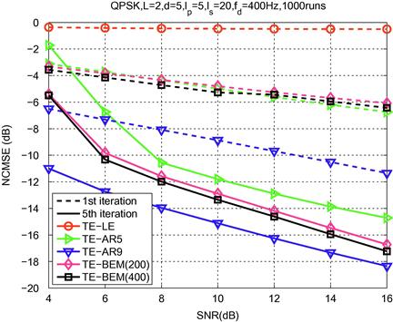
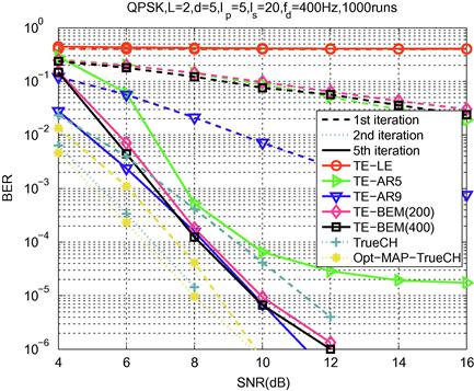
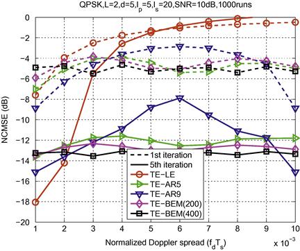
Figure 3.11 Turbo equalization: performance comparison for normalized Doppler spread (![]() )s under
)s under ![]() (20% training overhead).
(20% training overhead).
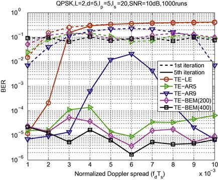
Figure 3.12 Turbo equalization: performance comparison for normalized Doppler spread (![]() )s under
)s under ![]() (20% training overhead).
(20% training overhead).
In Figures 3.10 and 3.12 the scheme TE-LE refers to the approach of [83] that uses the linear MMSE equalizer (e.g., [80]) coupled with modified RLS channel estimation. It is seen that this approach only works for normalized Doppler spread values of ![]() 0.002. In Figure 3.10 we also present the performance of the turbo equalizer based on the fixed-lag Kalman filter with knowledge of the true channel (curves with plus sign marker and labeled “TrueCH”) in order to illustrate the effectiveness of the proposed channel estimation approach; as there was little improvement beyond the second iteration, we only show the second iterative result with dotted curve labeled “TrueCH.” It is seen that there is a slightly more than 2 dB SNR penalty due to channel estimation. As has been noted in the literature, the Kalman filter based equalization is a sub-optimum equalizer compared to the trellis-based MAP (BCJR) equalizer [101]. In Figure 3.10 we present the performance of the turbo equalizer based on the optimum BCJR method with knowledge of the true channel (curves with asterisk marker and labeled “Opt-MAP-TrueCH”) in order to illustrate loss in performance due to suboptimality of the Kalman equalizer; as there was little improvement beyond the second iteration, we only show the second iterative result with dotted curve labeled “Opt-MAP-TrueCH”. It is seen that while there is a large difference in performance initially (see 1st iteration results for “TrueCH” and “Opt-MAP-TrueCH” where both are dashed curves with plus sign and asterisk markers, respectively), just one turbo iteration yields very close performance (see the two dotted curves). That is, at least for this example, performance loss in using Kalman equalizer instead of the BCJR equalizer is quite negligible.
0.002. In Figure 3.10 we also present the performance of the turbo equalizer based on the fixed-lag Kalman filter with knowledge of the true channel (curves with plus sign marker and labeled “TrueCH”) in order to illustrate the effectiveness of the proposed channel estimation approach; as there was little improvement beyond the second iteration, we only show the second iterative result with dotted curve labeled “TrueCH.” It is seen that there is a slightly more than 2 dB SNR penalty due to channel estimation. As has been noted in the literature, the Kalman filter based equalization is a sub-optimum equalizer compared to the trellis-based MAP (BCJR) equalizer [101]. In Figure 3.10 we present the performance of the turbo equalizer based on the optimum BCJR method with knowledge of the true channel (curves with asterisk marker and labeled “Opt-MAP-TrueCH”) in order to illustrate loss in performance due to suboptimality of the Kalman equalizer; as there was little improvement beyond the second iteration, we only show the second iterative result with dotted curve labeled “Opt-MAP-TrueCH”. It is seen that while there is a large difference in performance initially (see 1st iteration results for “TrueCH” and “Opt-MAP-TrueCH” where both are dashed curves with plus sign and asterisk markers, respectively), just one turbo iteration yields very close performance (see the two dotted curves). That is, at least for this example, performance loss in using Kalman equalizer instead of the BCJR equalizer is quite negligible.
2.03.7 Conclusion
A review of various approaches to channel estimation and equalization for communications systems was presented. Emphasis was on linear baseband equivalent models with a tapped delay line structure, and both time-invariant and time-variant (doubly-selective) models were discussed. Also emphasis was on basis expansion modeling for time-variant channels where the basis functions are related to the physical parameters of the channel (such as Doppler and delay spreads). Channel modeling was followed by a discussion of various approaches to channel estimation including training-based approaches, blind approaches, semi-blind approaches and superimposed training based approaches. Channel estimation approaches were followed by a discussion of channel equalization approaches including turbo-equalization for time-varying channels. A brief discussion of precoding was presented when the channel state information is available at the transmitter. We concluded the chapter with a discussion of channel tracking and combined data detection and channel tracking for time-varying channels. Channel tracking can be at block level suitable for block transmissions, or symbol-by-symbol level suitable for serial transmissions. Some of the approaches were illustrated via simulations.
Relevant Theory: Signal Processing Theory
See Vol. 1, Chapter 11 Parametric Estimation
See Vol. 1, Chapter 12 Adaptive Filters
References
1. Proakis J. Digital Communications. fourth ed. New York, NY: McGraw-Hill; 2001.
2. Bello P. Characterization of randomly time-variant channels. IEEE Trans Comm Syst. 1963;11:360–393.
3. Baddour KE, Beaulieu NC. Autoregressive modeling for fading channel simulation. IEEE Trans Wireless Commun. 2005;4:1650–1662.
4. Komninakis C, Fragouli C, Sayed A, Wesel R. Multi-input multi-output fading channel tracking and equalization using Kalman estimation. IEEE Trans Signal Process. 2002;50(5):1065–1076.
5. Li X, Wong T. Turbo equalization with nonlinear Kalman filtering for time-varying frequncy-selective fading channels. IEEE Trans Wireless Commun. 2007;6:691–700.
6. Kay SM. Modern Spectral Analysis: Theory and Application. Englewoods Cliffs, NJ: Prentice Hall; 1988.
7. Stoica P, Moses R. Spectral Analysis of Signals. Upper Saddle River, NJ: Pearson Prentice Hall; 2005.
8. Liu Z, Ma X, Giannakis G. Space-time coding and Kalman filtering for time-selective fading channels. IEEE Trans Commun. 2002;50:183–186.
9. Borah D, Hart B. Receiver structures for time-varying frequency-selective fading channels. IEEE J Sel Areas Commun. 1999;17:1863–1875.
10. Giannakis G, Tepedelenlioğlu C. Basis expansion models and diversity techniques for blind identification and equalization of time-varying channels. Proc IEEE. 1998;86:1969–1986.
11. Ma X, Giannakis G, Ohno S. Optimal training for block transmissions over doubly selective wireless fading channels. IEEE Trans Signal Process. 2003;51:1351–1366.
12. Sayeed A, Aazhang B. Joint multipath-doppler diversity in mobile wireless communications. IEEE Trans Commun. 1999;47:123–132.
13. Zemen T, Mecklenbräuker C. Time-variant channel estimation using discrete prolate spheroidal sequences. IEEE Trans Signal Process. 2005;53:3597–3607.
14. Leus G. On the estimation of rapidly time-varying channels. In: Proceedings of the European Signal Processing, Vienna, Austria. 2004;2227–2230.
15. Martone M. Wavelet-based separating kernels for array processing of cellular DS/CDMA signals in fast fading. IEEE Trans Commun. 2000;48:979–995.
16. Niedzwiecki M. Identification of Time-Varying Processes. New York, NY: Wiley; 2000.
17. Slepian D. Prolate spheroidal wave functions, Fourier analysis, and uncertainty—V: The discrete case. Bell Syst Tech J. 1978;57:1371–1430.
18. He S, Tugnait J. On bias-variance trade-off in superimposed training-based doubly selective channel estimation. In: Proceedings of the 2006 Conference on Information Systems and Sciences, Princeton University, NJ. 2006.
19. Baissas M-A, Sayeed A. Pilot-based estimation of time-varying multipath channels for coherent CDMA receivers. IEEE Trans Signal Process. 2002;50:2037–2049.
20. Kannu A, Schniter P. Capacity analysis of MMSE pilot-aided transmission for doubly selective channels. In: Proceedings of the 6th IEEE Workshop on Signal Processing Advances in Wireless, Communications. 2005;801–805.
21. Kannu A, Schniter P. MSE-optimal training for linear time-varying c.hannels. In: Proceedings of the 2005 IEEE Conference on Acoustics, Speech and Signal Processing, Philadelphia, PA. 2005;789–792.
22. Kannu A, Schniter P. Minimum mean-squared error pilot-aided transmision for MIMO doubly selective channels. In: Proceedings of the 2006 Conference on Information Systems & Sciences, Princeton University, NJ. 2006.
23. Leus G, Zhou S, Giannakis G. Orthogonal multiple access over time- and frequency-selective channels. IEEE Trans Inform theory. 2003;49:1942–1950.
24. Sayeed A, Sendonaris A, Aazhang B. Multiuser detection in fast-fading multipath environment. IEEE J Sel Areas Commun. 1998;16:1691–1701.
25. Gitlin R, Weinstein S. Fractionally-spaced equalization: an improved digital transversal equalizer. Bell Syst Tech J. 1981;60:275–296.
26. Gardner W. Introduction to Random Processes with Applications to Signals and Systems. New York, NY: McGraw-Hill; 1989.
27. Chen Y-C, Su Y. MIMO channel estimation in correlated fading environments. IEEE Trans Wireless Commun. 2010;9(3):1108–1119.
28. Karedal J, Almers P, Johansson A, Tufvesson F, Molisch A. A MIMO channel model for wireless personal area networks. IEEE Trans Wireless Commun. 2010;9(1):245–255.
29. Sayeed A. Deconstructing multiantenna fading channels. IEEE Trans Signal Process. 2002;50(10):2563–2579.
30. Shiu D, Foschini G, Gans M, Kahn J. Fading correlation and its effect on the capacity of multielement antenna systems. IEEE Trans Commun. 2000;48(3):502–513.
31. Weichselberger W, Herdin M, Ozcelik H, Bonek E. A stochastic MIMO channel model with joint correlation of both link ends. IEEE Trans Wireless Commun. 2006;5(3):90–100.
32. Cavers J. Pilot symbol assisted modulation and differential detection in fading and delay spread. IEEE Trans Commun. 1995;43:2206–2212.
33. Kaleh G, Vallet R. Joint parameter estimation and symbol detection for linear or nonlinear unknown dispersive channels. IEEE Trans Commun. 1994;42:2406–2413.
34. Krishnamurthy V, Moore J. On-line estimation of hidden Markov model parameters based on Kullback-Leibler information measure. IEEE Trans Signal Process. 1993;41:2557–2573.
35. Tong L, Perreau S. Multichannel blind channel estimation: from subspace to maximum likelihood methods. Proc IEEE. 1998;86:1951–1968.
36. Seshadri N. Joint data and channel estimation using blind trellis search techniques. IEEE Trans Commun. 1994;42:1000–1011.
37. Ghosh M, Weber C. Maximum-likelihood blind equalization. Optical Eng. 1992;31:1224–1228.
38. Raheli R, Polydoros A, Tzou C. Per-survivor processing: A general approach to MLSE in uncertain environments. IEEE Trans Commun. 1995;43:354–364.
39. Chugg K. Blind acquisition characteristics of PSP-based sequence detectors. IEEE J Sel Areas Commun. 1998;16:1518–1529.
40. Tugnait J. Blind estimation and equalization of digital communication FIR channels using cumulant matching. IEEE Trans Commun. 1995;43:1240–1245.
41. Tugnait J. Blind equalization and estimation of FIR communications channels using fractional sampling. IEEE Trans Commun. 1996;44:324–336.
42. Hatzinakos D, Nikias C. Blind equalization using a tricepstrum based algorithm. IEEE Trans Commun. 1991;39:669–681.
43. Vidal J, Fonollosa J. Adaptive blind equalization using weighted cumulant slices. Int J Adapt Control Signal Process. 1996;10:213–238.
44. Tugnait J. Channel estimation and equalization using higher-order statistics. In: Upper Saddle River, NJ: Prentice Hall; 2001;1–39. Giannakis G, Hua Y, Stoica P, Tong L, eds. Signal Processing Advances in Wireless and Mobile Communications, Trends in Channel Estimation and Equalization. vol. I.
45. Tong L, Xu G, Kailath T. A new approach to blind identification and equalization of multipath channels. IEEE Trans Inform Theory. 1994;40:340–349.
46. Tugnait J. On blind identifiability of multipath channels using fractional sampling and second-order cyclostationary statistics. IEEE Trans Inform Theory. 1995;41:308–311.
47. de Carvalho E, Slock D. Stochastic maximum likelihood methods for semi-blind channel estimation. In: Upper Saddle River, NJ: Prentice Hall; 2001;Giannakis G, Hua Y, Stoica P, Tong L, eds. Signal Processing Advances in Wireless and Mobile Communications. vol. I Chapter 7.
48. Cirpan H, Tsatsanis M. Stochastic maximum likelihood methods for semi-blind channel estimation. IEEE Signal Proc Lett. 1998;5:21–24.
49. Laurila J, Kopsa K, Bonek E. Semi-blind signal estimation for smart antennas using subspace tracking. In: Proceedings of the IEEE Workshop on Signal Processing Advances in Wireless Communications, Annapolis, MD. 1999.
50. Gorokhov A, Loubaton P. Semi-blind second order identification of convolutive channels. In: Proceedings of the 1997 IEEE Conference on Acoustics, Speech and Signal Processing, Munich, Germany. 1997;3905–3908.
51. Lasaulce S, Loubaton P, Moulines E. A semi-blind channel estimation technique based on second-order blind method for CDMA systems. IEEE Trans Signal Process. 2003;51:1894–1904.
52. Hoeher P, Tufvesson F. Channel estimation with superimposed pilot sequence. In: Proceedings of the IEEE Global Communications Conference, Rio de Janeiro, Brazil. 1999;2162–2166.
53. Holden T, Feher K. A spread spectrum based system technique for synchronization of digital mobile communication system. IEEE Trans Broadcast. 1990;36:185–194.
54. Mazzenga F. Channel estimation and equalization for M-QAM transmission with a hidden pilot sequence. IEEE Trans Broadcast. 2000;46:170–176.
55. Ghogho M, McLernon D, Alamdea-Hernandez E, Swami A. Channel estimation and symbol detection for block transmission using data-dependent superimposed training. IEEE Signal Proc Lett. 2005;12:226–229.
56. Ghogho M, McLernon D, Alamdea-Hernandez E, Swami A. SISO and MIMO channel estimation and symbol detection using data-dependent superimposed training. In: Proceedings of the IEEE Conference on Acoustics, Speech and Signal Processing, PA, Philadelphia. 2005;III-461–III-464.
57. Tugnait J, He S. Doubly-selective channel estimation using data-dependent superimposed training and exponential bases models. In: Proceedings of the Conf on Information Systems and Sciences, Princeton University, NJ. 2006.
58. Tugnait J, He S. Multiuser/MIMO doubly selective fading channel estimation using superimposed training and Slepian sequences. IEEE Trans Veh Technol. 2010;59:1341–1354.
59. Holma H, Toskala AE. WCDMA for UMTS: Radio Access for Third Generation Mobile Communications. second ed. New York, NY: Wiley; 2002.
60. Orozco-Lugo A, Lara M, McLernon D. Channel estimation using implicit training. IEEE Trans Signal Proc. 2004;52:240–254.
61. Tugnait J, Luo W. On channel estimation using superimposed training and first-order statistics. In: Proceedings of the, IEEE Conference on Acoustics, Speech and Signal Processing, Hong Kong. 2003.
62. Tugnait J, Luo W. On channel estimation using superimposed training and first-order statistics. IEEE Commun Lett. 2003;8:413–415.
63. Zhou G, Viberg M, McKelvey T. A first-order statistical method for channel estimation. IEEE Signal Process Lett. 2003;10:57–60.
64. Dong M, Tong L, Sadler B. Optimal insertion of pilot symbols for transmissions over time-varying flat fading channels. In: Proceedings of the 2003 IEEE Workshop on Signal Processing Advances in Wireless Communications, Rome, Italy. IEEE 2003;472–476.
65. Biguesh M, Gershman A. Training-based MIMO channel estimation: a study of estimator tradeoffs and optimal training signals. IEEE Trans Signal Proc. 2006;54(3):884–893.
66. Ma X, Yang L, Giannakis G. Optimal training for MIMO frequency-selective fading channels. IEEE Trans Wireless Commun. 2005;4(2):453–466.
67. Barhumi I, Leus G, Moonen M. Time-varying FIR equalization for doubly selective channels. IEEE Trans Wireless Commun. 2005;4(1):202–214.
68. Song L, Tugnait J. Doubly-selective fading channel equalization: A comparison of the Kalman filter approach with the basis expansion model-based equalizers. IEEE Trans Wireless Commun. 2009;8(1):60–65.
69. Al-Dhahir N, Cioffi JM. MMSE decision-feedbck equalizers: finite-length results. IEEE Trans Inf Theory. 1995;41(4):961–975.
70. Sayed AH. Fundamentals of Adaptive Filtering. New York, NY: Wiley; 2003.
71. Stüber GL. Principles of Mobile Communication. second ed. Boston, MA: Kluwer; 2002.
72. Forney G. Maximum-likelihood sequence estimation of digital sequences in the presence of intersymbol interference. IEEE Trans Inform Theory. 1972;18:363–378.
73. Lin S, Costello JJ. Error Control Coding. Englewood Cliffs, NJ: Prentice-Hall; 1983.
74. Bahl L, Cocke J, Jelinek F, Raviv J. Optimal decoding of linear codes for minimizing symbol error rate. IEEE Trans Inform Theory. 1974;20:284–287.
75. Tuchler M, Singer A. Turbo equalization: an overview. IEEE Trans Inform theory. 2011;70(2):920–952.
76. Berrou C, Glavieux A, Thitimajshima P. Near Shannon limit error-correcting coding and decoding: turbo codes. In: Proceedings of IEEE Int Conf on Commun., Geneva, Switzerland. 1993.
77. Douillard C, Jézéquel M, Berrou C, Picart A, Didier P, Glavieux A. Iterative correction of intersymbol interference: turbo-equalization. Eur Trans Telecommun. 1995;6:507–511.
78. Anastassopoulos A, Chugg K. Iterative equalization/decoding for TCM for frequency-selective channels. In: Proceedings of the 1997 Asilomar Conf on Signals, Systems, Compueters, Pcific Grove, CA. 1997;177–181.
79. Wang X, Poor H. Iterative (turbo) soft interference cancellation and decoding for coded CDMA. IEEE Trans Commun. 1999;47(7):1046–1061.
80. Tuchler M. Minimum mean squared error equalization using a priori information. IEEE Trans Signal Process. 2002;50(3):673–683.
81. Tuchler M. Turbo equalization: principles and new results. IEEE Trans Commun. 2002;50(5):754–767.
82. Nissilä M, Pasupathy S. Adaptive Bayesian and EM-based detectors for frequency-selective fading channels. IEEE Trans Commun. 2003;51:1325–1336.
83. Otnes R, Tuchler M. Iterative channel estimation for turbo equalization for time-varying frequency-selective channels. IEEE Trans Wireless Commun. 2004;3:1918–1923.
84. Song S, Singer A, Sung K. Soft input channel estimation for turbo equalization. IEEE Trans Signal Process. 2004;52:2885–2894.
85. Kim H, Tugnait J. Turbo equalization for doubly-selective fading channels using nonlinear Kalman filtering and basis expansion models. IEEE Trans Wireless Commun. 2010;9:2076–2087.
86. Harashima H, Miyakawa H. Matched-transmission technique for channels with intersymbol interference. IEEE Trans Commun. 1972;20:774–780.
87. Kuo JC-C, Tsai S-O, Tadjpour L, Chang Y-H. Precoding Techniques for Digital Communication Systems. New York, NY: Springer; 2008.
88. Tomlinson M. New automatic equalizer employing modulo arithmetic. Electron Lett. 1971;7:138–139.
89. Forney G, Eyuboglu M. Combined equalization and coding using precoding. IEEE Commun Mag. 1991;29:25–34.
90. Vu M, Paulraj A. MIMO wireless linear precoding. IEEE Signal Proc Mag. 2007;24(5):86–105.
91. Scaglione A, Stoica P, Barbarossa S, Giannakis G, Sampath H. Optimal designs for space-time linear precoders and decoders. IEEE Trans Signal Process. 2002;50:1051–1063.
92. Liu T, Zhang J-K, Wong K. Optimal precoder design for correlated MIMO communication systems using zero-forcing decision feedback equalization. IEEE Trans Signal Proc. 2009;57:3600–3612.
93. Su W, Zheng W, Chai L. Precoder design and blind channel identification of MIMO channels. IEEE Trans Signal Process. 2006;54(7):2725–2736.
94. Wang Z, Giannakis G. Block precoding for MUI/ISI-resilient generalized multicarrier CDMA with multirate capabilities. IEEE Trans Commun. 2001;49(11):2016–2027.
95. Tugnait J, He S, Kim H. Doubly-selective channel estimation using exponential basis models and subblock tracking. IEEE Trans Signal Process. 2010;58:1275–1289.
96. Li X, Ritcey J. Bit-interleaved coded modulation with iterative decoding. In: Proceedings of IEEE International Conference, Communication. 1999;858–864.
97. Lopes R, Berry J. The soft-feedback equalizer for turbo equalization of highly dispersive channels. IEEE Trans Commun. 2006;54(5):783–788.
98. Vogelbruch F, Haar S. Low complexity turbo equalization based on soft feedback interference cancelation. IEEE Commun Lett. 2005;9(7):586–588.
99. Wang X, Poor H. Wireless Communication Systems: Advanced Techiques for Signal Reception. Upper Saddle River, NJ: Prentice Hall; 2004.
100. Zheng Y, Xiao C. Simulation models with correct statistical properties for Rayleigh fading channels. IEEE Trans Commun. 2003;51:920–928.
101. Koetter R, Singer A, Tuchler M. Turbo equalization. IEEE Signal Proc Mag. 2004;21:67–80.