
Optimal Radar Waveform Design
Joseph R. Guerci, Guerci Consulting LLC, Vienna, VA, USA, [email protected]
Abstract
A confluence of steady advances in radar enabling technologies, and ever increasing demands on radar performance in challenging environments, has afforded a re-examination of the fundamental theoretical framework upon which classical waveform design is based. For example, the advent of “digital radar” (e.g., solid state amplifiers, digital arbitrary waveform generators (DAWGs), etc.) allows for a far greater level of waveform diversity than has previously been the case. Major advances in high performance embedded computing (HPEC) including general purpose graphical processing units (GPUs), have allowed for the inclusion of sophisticated knowledge-aided (KA) processing techniques such as those beginning with the DARPA/AFRL KASSPER project. Lastly, ever-increasing demands on radar performance in challenging environments have forced design engineers to stretch performance wherever possible. In this tutorial, an optimal multi-input multi-output (MIMO) formulation is presented from first principles that leverages all of the aforementioned enabling technologies. The formulation allows for the joint optimization of the transmit-receive functions for maximizing detection and/or target identification (ID) as a function of the target channel characteristics.
Keywords
Adaptive waveform diversity; Optimal MIMO waveform; Knowledge-aided (KA) processing; Fully adaptive radar; Cognitive radar; Optimal target ID
Nomenclature
![]()
![]() -dimensional complex vector space
-dimensional complex vector space
![]() multidimensional transmit signal
multidimensional transmit signal
![]() multidimensional target transfer function (generally stochastic)
multidimensional target transfer function (generally stochastic)
![]() multidimensional received target “Echo”
multidimensional received target “Echo”
![]() multidimensional complex additive receiver noise (zero mean)
multidimensional complex additive receiver noise (zero mean)
![]() additive receiver noise covariance matrix
additive receiver noise covariance matrix
![]() clutter channel transfer function (generally stochastic)
clutter channel transfer function (generally stochastic)
2.14.1 Introduction
Adaptive processing has long been implemented in the receive chain of radar, beginning with automatic gain control (AGC), cell-averaging constant false alarm rate (CA-CFAR) [1] and culminating in today’s space-time adaptive processing (STAP) [2]. However, adaptivity in the transmit chain is virtually nonexistent, save for mode adaptivity (such as switching in different nonadaptive waveforms such as pulse repetition frequency (PRF) and bandwidth) and adaptive spectral notching to address narrowband interference mitigation. Historically, the reasons for the lack of transmit adaptivity included:
• Inability of radar hardware to transmit arbitrary waveforms (or more generally arbitrary space-time waveforms).
• Lack of sufficient embedded computing to allow for real-time waveform adaptation.
• As a result of the above, there is a lack of basic theory for optimal waveform design as a function of the target-interference channel (except for very specialized cases).
However, as discussed in the abstract, the first two obstacles are no longer the case. All that remains is to revisit the basic radar theoretic problem and derive a new set of design equations allowing for transmit adaptivity as a function of the target-interference channel.
This chapter develops the basic theory of optimal transmit/receive design using a multi-input, multi-output (MIMO) formulation that can account for all potential degrees of freedom (DOFs) such as waveform (fast-time), angle, and polarization. Various applications and examples are provided to further illustrate the potential impact of joint transmit/receive adaptivity. The only mathematical prerequisites for this material is a basic understanding of matrix algebra, basic optimization theory, and stochastic processes.
2.14.2 Optimum transmit-receiver design for the additive colored noise case: detection
Due to the finite bandwidth constraint for all real-world radars, there is no loss in generality in invoking Shannon’s sampling theory [3]. This, in turn, allows for a matrix algebra formulation of the basic radar interaction equations which both significantly eases nomenclature and exposition (see below).
Consider the basic radar block diagram in Figure 14.1. A generally complex-valued and multidimensional transmit signal, ![]() , (i.e., an N-dimensional multi-input (MI) signal), interacts with a target denoted by the target transfer matrix
, (i.e., an N-dimensional multi-input (MI) signal), interacts with a target denoted by the target transfer matrix ![]() . The resulting M-dimensional multi-output (MO) signal (echo),
. The resulting M-dimensional multi-output (MO) signal (echo), ![]() , is then received along with ACN
, is then received along with ACN ![]() , assumed to be zero mean, wide sense stationary, with corresponding complex valued covariance
, assumed to be zero mean, wide sense stationary, with corresponding complex valued covariance ![]() . The vector-matrix formulation is completely general inasmuch as any combination of spatial and temporal dimensions can be represented.
. The vector-matrix formulation is completely general inasmuch as any combination of spatial and temporal dimensions can be represented.
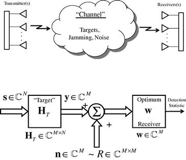
Figure 14.1 Fundamental multichannel radar block diagram for the ACN case. The objective is to design both the transmit and receive functions to maximize the output SINR given the channel characteristics.
For example, the N-dimensional input vector s could represent the N complex (i.e., in-phase/quadrature, or “ I and Q” [4]) samples of a single-channel transmit waveform ![]() , that is,
, that is,
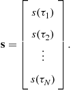 (14.1)
The corresponding target transfer matrix, ![]() , would thus contain the corresponding samples of the complex target impulse response,
, would thus contain the corresponding samples of the complex target impulse response, ![]() , which for the causal linear time-invariant (LTI) case would have the form [3]
, which for the causal linear time-invariant (LTI) case would have the form [3]
 (14.2)
Without loss of generality we have assumed uniform time sampling, that is, ![]() , where T is a suitably chosen sampling interval [5]. Note also that for convenience and a significant reduction in mathematical nomenclature overhead,
, where T is a suitably chosen sampling interval [5]. Note also that for convenience and a significant reduction in mathematical nomenclature overhead, ![]() is used, (i.e., the same number of transmit and receive DOFs). The reader is encouraged to, where desired, reinstate the inequality and confirm that the underlying equations derived throughout this chapter have the same basic form except for differing vector and matrix dimensionalities. Also it should be noted that in general
is used, (i.e., the same number of transmit and receive DOFs). The reader is encouraged to, where desired, reinstate the inequality and confirm that the underlying equations derived throughout this chapter have the same basic form except for differing vector and matrix dimensionalities. Also it should be noted that in general ![]() is stochastic.
is stochastic.
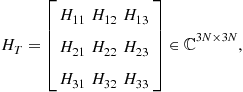
The formalism is readily extensible to the multiple-transmitter, multiple-receiver case. For example, if there are three independent transmit/receive channels (e.g., an AESA), then the input vector s of Figure 14.1 would have the form
 (14.3)
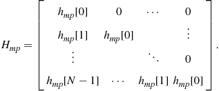
where ![]() denotes the samples (as in (14.1)) of the transmitted waveform out of the ith transmit channel. The corresponding target transfer matrix would in general have the form
denotes the samples (as in (14.1)) of the transmitted waveform out of the ith transmit channel. The corresponding target transfer matrix would in general have the form
 (14.4)
where the submatrix ![]() is the transfer matrix between the ith receive and jth transmit channels for all time samples of the waveform. These examples make clear that the matrix-vector, input-output formalism is completely universal and can accommodate whatever transmit/receive DOF configuration desired.
is the transfer matrix between the ith receive and jth transmit channels for all time samples of the waveform. These examples make clear that the matrix-vector, input-output formalism is completely universal and can accommodate whatever transmit/receive DOF configuration desired.
Returning to Figure 14.1, we now wish to jointly optimize the transmit/receive functions to maximize output SINR, which under the Gaussian assumption, would yield a sufficient statistic that maximizes the probability of detection for a prescribed false alarm rate [6]. We will find it convenient to work backward: to begin by optimizing the receiver as a function of the input and then finally optimizing the input and thus the overall output SINR.
For any finite norm input s, the receiver that maximizes output SINR for the ACN case is the so-called whitening (or colored noise) matched filter, as shown in Figure 14.2 [6]. Note that for the additive Gaussian colored noise (AGCN) case, this receiver is also statistically optimum [6].
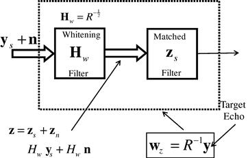
Figure 14.2 The optimum (max SINR) receiver for the ACN case consists of a whitening filter followed by a white noise matched filter.
![]() , which denotes the total interference covariance matrix associated with n, is further assumed to be independent of s and Hermitian positive definite [7] (guaranteed in practice due to ever-present receiver noise [6]), then the corresponding whitening filter shown in Figure 14.2 is given by [6]:
, which denotes the total interference covariance matrix associated with n, is further assumed to be independent of s and Hermitian positive definite [7] (guaranteed in practice due to ever-present receiver noise [6]), then the corresponding whitening filter shown in Figure 14.2 is given by [6]:
![]() (14.5)
(14.5)
where the superscript ![]() denotes the “matrix square root inverse” [8].
denotes the “matrix square root inverse” [8].
The output of the linear whitening filter, ![]() , will consist of signal and noise components,
, will consist of signal and noise components, ![]() , respectively, given by
, respectively, given by
![]() (14.6)
(14.6)
![]()
where ![]() denotes the target echo as shown in Figure 14.2 (i.e., the output of
denotes the target echo as shown in Figure 14.2 (i.e., the output of ![]() .
.
Since the noise has been whitened via a linear—in this case full-rank—transformation [6]), the final receiver stage consists of a white noise matched filter of the form (to within a multiplicative scalar)
![]() (14.7)
(14.7)
The corresponding output SNR is thus given by
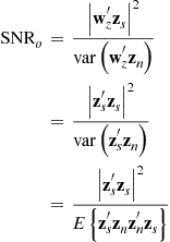 (14.8)
where superscript “![]() ” denotes complex conjugate transpose, and
” denotes complex conjugate transpose, and ![]() denotes the variance operator. Note that due to the whitening operation
denotes the variance operator. Note that due to the whitening operation ![]() .
.
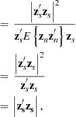
In words, the output SNR is proportional to the energy in the whitened target echo. This fact is key to optimizing the input function: Chose s (the input) to maximize the energy in the whitened target echo:
![]() (14.9)
(14.9)
Substituting ![]() into (14.9) yields the objective function that explicitly depends on the input
into (14.9) yields the objective function that explicitly depends on the input
![]() (14.10)
(14.10)
where
![]() (14.11)
(14.11)
Recognizing that (14.10) involves the magnitude of the inner product of two vectors s and ![]() , we readily have from the Cauchy-Schwarz theorem [9] the condition that s must satisfy to yield a maximum, namely, smust be collinear with
, we readily have from the Cauchy-Schwarz theorem [9] the condition that s must satisfy to yield a maximum, namely, smust be collinear with![]() :
:
![]() (14.12)
(14.12)
In other words, the optimum input ![]() must be an eigenvector of
must be an eigenvector of ![]() with associated maximum eigenvalue.
with associated maximum eigenvalue.
The previous set of input-output design equations represents the absolute optimum that any combination of transmit/receive operations can achieve and thus are fundamentally important in ascertaining the value of advanced adaptive methods (e.g., adaptive waveforms, transmit/receive beamforming). Note also that (14.12) can be generalized to the case where the target response is random:
![]() (14.13)
(14.13)
In this case, ![]() maximizes the expected value of the output SINR.
maximizes the expected value of the output SINR.
Next we illustrate the application of the previously given optimum design equations to the additive colored noise problem arising from a broadband multipath interference source.
2.14.2.1 Application to broadband multipath interference
This application illustrates the optimum transmit/receive configuration for maximizing output SINR in the presence of colored noise interference arising from a multipath broadband noise source. More specifically, for the single transmit/receive channel case, it derives the optimum transmit pulse modulation (i.e., pulse shape/spectrum).
Figure 14.3 illustrates a nominally broadband white noise source undergoing a series of multipath scatterings that in turn colors the noise spectrum [10]. Assuming (for simplicity) that the multipath reflections are dominated by several discrete specular reflections, the resultant signal can be viewed as the output of a causal tapped delay line filter (i.e., an FIR filter [3]) of the form
![]() (14.14)
(14.14)
that is driven by white noise. The corresponding input-output transfer ![]() is thus given by
is thus given by
 (14.15)

Figure 14.3 Illustration of colored noise interference resulting from a broadband (i.e., white noise) source undergoing strong discrete multipath reflections. The resulting signal can be approximated as white noise driving a finite impulse response (FIR) filter.
In terms of the multipath transfer matrix, ![]() , the colored noise interference covariance matrix is given by
, the colored noise interference covariance matrix is given by
 (14.16)
![]()
where the driving white noise source ![]() is a zero mean complex vector random variable with an identity covariance matrix:
is a zero mean complex vector random variable with an identity covariance matrix:
![]() (14.17)
(14.17)
Assuming a unity gain point target at the origin, that is, ![]() , yields a target transfer matrix
, yields a target transfer matrix ![]() given by
given by
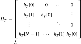 (14.18)
While certainly a more complex (and thus realistic) target model could be assumed, we wish to focus on the impact the colored noise has on shaping the optimum transmit pulse. We will introduce more complex target response models in the target ID section.
Figure 14.4 shows the in-band interference spectrum for the case when ![]() , all other coefficients are set to zero. The total number of fast-time (range bin) samples was set to both a short-pulse case of
, all other coefficients are set to zero. The total number of fast-time (range bin) samples was set to both a short-pulse case of ![]() (Figure 14.4a) and a long-pulse case of
(Figure 14.4a) and a long-pulse case of ![]() (Figure 14.4b). Note that the multipath colors the otherwise flat noise spectrum. Also displayed is the spectrum of a conventional (and thus non-optimized) LFM pulse with a time-bandwidth product,
(Figure 14.4b). Note that the multipath colors the otherwise flat noise spectrum. Also displayed is the spectrum of a conventional (and thus non-optimized) LFM pulse with a time-bandwidth product, ![]() , of 5 (Figure 14.4a) and 50 (Figure 14.4b), respectively [11,12].
, of 5 (Figure 14.4a) and 50 (Figure 14.4b), respectively [11,12].

Figure 14.4 Spectra of the colored noise interference along with conventional and optimal pulse modulations. (a) Short-pulse case where total duration for the LFM and optimum pulse are set to 11 range bins (fast-time taps). (b) Long-pulse case where total duration for the LFM and optimum pulse are set to 100 range bins. Note that in both cases the optimum pulse attempts to anti-match to the colored noise spectrum under the frequency resolution constraint set by the total pulse width.
Given R from (14.16), the corresponding whitening filter ![]() is given by
is given by
![]() (14.19)
(14.19)
Combining (14.19) with (14.18), the total composite channel transfer matrix H is thus given by
![]() (14.20)
(14.20)
Substituting (14.20) into (14.12) yields
![]() (14.21)
(14.21)
That is, the optimum transmit waveform is the maximum eigenvector associated with the inverse of the interference covariance matrix.
Displayed in Figures 14.4a and 14.4b are the spectra of the optimum transmit pulses obtained by solving (14.21) for the maximum eigenfunction-eigenvalue pair for the aforementioned short- and long-pulse cases, respectively. Note how the optimum transmit spectrum naturally emphasizes portions of the spectrum where the interference is weak—which is an intuitively satisfying result.
The SINR gain of the optimum short pulse, ![]() , relative to that of a nonoptimized chirp pulse,
, relative to that of a nonoptimized chirp pulse, ![]() , is
, is
![]() (14.22)
(14.22)
while for the long-pulse case
![]() (14.23)
(14.23)
The increase in SINR for the long-pulse case is to be expected since it has finer spectral resolution and can therefore more precisely shape the transmit modulation to “anti-match” the interference. Of course, the unconstrained optimum pulse has certain practical deficiencies (e.g., poorer resolution, compression sidelobes) compared with a conventional pulse. We will revisit these issues when constrained optimization is introduced.
This application is similar in spirit to the spectral notching waveform design problem that arises when strong co-channel narrowband interferers are present [13]. In this case it is desirable not only to filter out the interference on receive but also to choose a transmit waveform that minimizes energy in the co-channel bands. The reader is encouraged to experiment with different notched spectra and pulse length assumptions and to apply (14.12) as indicated. Non-impulsive target models can also be readily incorporated.
2.14.3 Optimum transmit-receiver design for the clutter case: detection
Radar clutter refers to all unwanted reflections emanating from anything other than the desired target of interest [12]. It is thus a form of transmit-signal dependent interference, in contrast to the previously considered ACN case. Unfortunately, the joint optimization of the transmit and receive functions for the general additive colored noise plus clutter (signal-dependent noise) has been shown to result in a highly nonlinear problem [14] (though efficient iterative methods have been developed to solve these equations [14]). In practice, however, there is often a natural “separation principle” between additive colored noise (signal independent) and clutter (signal dependent). For example, narrowband electromagnetic interference (EMI) resulting from co-channel interference might require fast-time receiver and transmit spectral notching [13], leaving the slow-time or spatial DOF available for clutter suppression. Similarly, adaptive beamforming for broadband jammer nulling can be separated from the clutter suppression problem in a two-stage approach (see, e.g., [15]). We will thus concentrate in this section on the clutter dominant case and focus solely on maximizing the output signal-to-clutter ratio (SCR).
Unlike the previous additive colored noise case, clutter (i.e., channel reverberations) is a form of signal-dependent noise [16,17] since the clutter returns depend on the transmit signal characteristics (e.g., transmit antenna pattern and strength, operating frequencies, bandwidths, polarization). Referring to Figure 14.5, the corresponding SCR at the input to the receiver is given by
 (14.24)
where ![]() denotes the clutter transfer matrix, which is generally taken to be stochastic. Equation (14.24) is a generalized Rayleigh quotient [7] that is maximized when s is a solution to the generalized eigenvalue problem
denotes the clutter transfer matrix, which is generally taken to be stochastic. Equation (14.24) is a generalized Rayleigh quotient [7] that is maximized when s is a solution to the generalized eigenvalue problem
![]() (14.25)
(14.25)
with corresponding maximum eigenvalue. When ![]() is positive definite, (14.25) can be converted to an ordinary eigenvalue problem of the form we have already encountered, specifically,
is positive definite, (14.25) can be converted to an ordinary eigenvalue problem of the form we have already encountered, specifically,
![]() (14.26)
(14.26)

Figure 14.5 Radar signal block diagram for the clutter dominant case illustrating the direct dependency of the clutter signal on the transmitted signal.
2.14.3.1 Application: sidelobe clutter discrete suppression
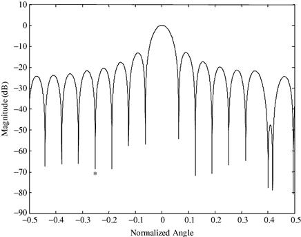
Consider a narrowband N = 16 element uniform linear array (ULA) with half-wavelength interelement spacing with a boresight pointing quiescent pattern (see Figure 14.6) [18]. In addition to the desired target at a normalized angle of ![]() (array boresight), there are strong sidelobe targets at
(array boresight), there are strong sidelobe targets at ![]() , where a normalized angle is defined as
, where a normalized angle is defined as
![]() (14.27)
(14.27)
In (14.27) d is the interelement spacing of the ULA, and ![]() is the operating wavelength (consistent units and narrowband operation assumed).
is the operating wavelength (consistent units and narrowband operation assumed).
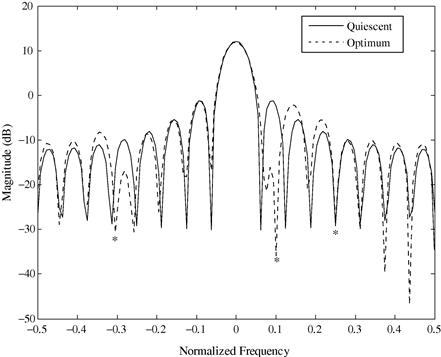
Figure 14.6 Illustration of proactive sidelobe target blanking on transmit achieved by maximizing the SCR. Note the presence of nulls in the directions of competing targets while preserving the desired mainbeam response.
The presence of these targets (possibly large clutter discretes) could have been previously detected, thus making their AOAs known. Also, their strong sidelobes could potentially mask weaker mainlobe targets. With this knowledge, it is desired to minimize any energy from these targets leaking into the mainbeam detection of the target of interest by nulling on transmit, or placing transmit antenna pattern nulls in the directions of the unwanted targets.
For the case at hand, the (m, n)th elements of the target and interferer transfer matrices are given, respectively, by
![]() (14.28)
(14.28)
![]() (14.29)
(14.29)
where ![]() is an overall bulk delay (two way propagation) that does not affect the solution to (14.25) and will thus be subsequently ignored, and
is an overall bulk delay (two way propagation) that does not affect the solution to (14.25) and will thus be subsequently ignored, and ![]() is the (m, n)th element of the clutter transfer matrix and consists of the linear superposition of the three target returns resulting from transmitting a narrowband signal from the nth transmit element and receiving it on the mth receive element of a ULA that uses the same array for transmit and receive [2,12]. Note that in practice there would be a random relative phase between the signals in (14.29), which for convenience we have ignored but which can easily be accommodated by taking the expected value of the kernel
is the (m, n)th element of the clutter transfer matrix and consists of the linear superposition of the three target returns resulting from transmitting a narrowband signal from the nth transmit element and receiving it on the mth receive element of a ULA that uses the same array for transmit and receive [2,12]. Note that in practice there would be a random relative phase between the signals in (14.29), which for convenience we have ignored but which can easily be accommodated by taking the expected value of the kernel ![]() .
.
Solving (14.25) for the optimum eigenvector yields the transmit pattern that maximizes the SCR, which is the pattern also displayed in Figure 14.6. The competing target amplitudes were set to 40 dB relative to the desired target and 0 dB of diagonal loading was added to ![]() to improve numerical conditioning and allow for its inversion. Although this is somewhat arbitrary, it does provide a mechanism for controlling null depth, that in practice is limited by the amount of transmit channel mismatch [19]. Note the presence of transmit antenna pattern nulls in the directions of the competing targets as desired.
to improve numerical conditioning and allow for its inversion. Although this is somewhat arbitrary, it does provide a mechanism for controlling null depth, that in practice is limited by the amount of transmit channel mismatch [19]. Note the presence of transmit antenna pattern nulls in the directions of the competing targets as desired.
An important caveat to the above was the assumption of perfect knowledge of the transmit array manifold—that is the assumption of a perfectly transmit calibrated AESA. This can only approximately be the case in practice. Indeed knowledge of the receive array manifold, which is generally easier to estimate on-the-fly, is not equivalent to that of the transmit manifold (since slightly different electrical pathways are taken). A MIMO method has been developed for transmit manifold calibration under the DARPA ISAT program and can be found in [20].
2.14.3.2 Application: optimum pulse shaping for maximizing SCR
In this simple example, we rigorously verify an intuitively obvious result regarding pulse shape and detecting a point target in uniform clutter: the best waveform for detecting a point target in distributed i.i.d clutter is itself an impulse (i.e., a waveform with maximal resolution), a well-known result rigorously proven by Manasse [21] using a different method.
Consider a unity point target, arbitrarily chosen to be at the temporal origin. Its corresponding impulse response and transfer matrix are respectively given by
![]() (14.30)
(14.30)
and
![]() (14.31)
(14.31)
where ![]() denotes the
denotes the ![]() identity matrix. For uniformly distributed clutter, the corresponding impulse response is of the form
identity matrix. For uniformly distributed clutter, the corresponding impulse response is of the form
 (14.32)
where ![]() denotes the complex reflectivity random variable of the clutter contained in the ith range cell (i.e., fast-time tap). The corresponding transfer matrix is given by
denotes the complex reflectivity random variable of the clutter contained in the ith range cell (i.e., fast-time tap). The corresponding transfer matrix is given by
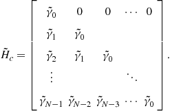 (14.33)
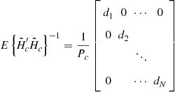
Assuming that the ![]() values are i.i.d., we have
values are i.i.d., we have
![]() (14.34)
(14.34)
and thus
 (14.35)
where ![]() denotes the (i, j)th element of the transfer matrix. Note that (14.35) is also diagonal (and thus invertible), but with non-equal diagonal elements.
denotes the (i, j)th element of the transfer matrix. Note that (14.35) is also diagonal (and thus invertible), but with non-equal diagonal elements.
Finally, substituting (14.31) and (14.35) into (14.26) yields
![]() (14.36)
(14.36)
where
 (14.37)
and
![]() (14.38)
(14.38)
It is readily verified that the solution to (14.36) yielding the maximum eigenvalue is given by
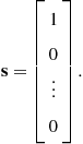 (14.39)
Thus the optimum pulse shape for detecting a point target is itself an impulse. This should be immediately obvious since it is the shape that excites the range bin only with the target and zeros out all other range bin returns that contain competing clutter.
Of course, transmitting a short pulse (much less an impulse) is problematic in the real world (e.g., creating extremely high peak power pulses) thus an approximation to a short pulse in the form of a spread spectrum waveform (e.g., LFM) is often employed [11]. This example also makes clear that in uniform random clutter nothing is gained by sophisticated pulse shaping for a point target other than to maximize bandwidth (i.e., range resolution) [21]. The interested reader is referred to [22] for further examples of optimizing other DOF (e.g., angle-Doppler) for the clutter mitigation problem.
Up to this point we have been focused on judiciously choosing the transmit/receive DOF to maximize SINR or SCR (and thus ultimately detection). In the next section we will extend this framework to the target identification problem.
2.14.4 Optimizing the transmit-receive functions for target identification
Consider the problem of determining target type when two possibilities exist (the multitarget case is addressed later in this section). This can be cast as a classical binary hypothesis testing problem [6]:
![]() (14.40)
(14.40)
where ![]() denote the target transfer matrices for targets 1 and 2, respectively. For the AGCN case, the well-known optimum receiver decision structure consists of a bank of matched filters (generally whitening matched filters), each tuned to a different target assumption, followed by comparator as shown in Figure 14.7[6]. Note that (14.40) presupposes that either Target 1 or 2 is present, but not both. Also, it has been tacitly assumed that a binary detection test has been conducted to ensure that a target is indeed present [6]. Alternatively, the null hypothesis (no target present) can be included in the test as a separate hypothesis (see below).
denote the target transfer matrices for targets 1 and 2, respectively. For the AGCN case, the well-known optimum receiver decision structure consists of a bank of matched filters (generally whitening matched filters), each tuned to a different target assumption, followed by comparator as shown in Figure 14.7[6]. Note that (14.40) presupposes that either Target 1 or 2 is present, but not both. Also, it has been tacitly assumed that a binary detection test has been conducted to ensure that a target is indeed present [6]. Alternatively, the null hypothesis (no target present) can be included in the test as a separate hypothesis (see below).

Figure 14.8 illustrates the situation at hand. If Target-1 is present, the observed signal ![]() will tend to cluster about the #1 point in observation space—which could include any number of dimensions relevant to the target ID problem (e.g., fast-time, angle, Doppler, polarization). The uncertainty sphere (generally ellipsoid for ACN case) surrounding #1 in Figure 14.7 represents the 1-sigma probability for the additive noise
will tend to cluster about the #1 point in observation space—which could include any number of dimensions relevant to the target ID problem (e.g., fast-time, angle, Doppler, polarization). The uncertainty sphere (generally ellipsoid for ACN case) surrounding #1 in Figure 14.7 represents the 1-sigma probability for the additive noise ![]() —and similarly for #2. Clearly, if
—and similarly for #2. Clearly, if ![]() and
and ![]() are relatively well separated, the probability of correct classification is commensurately high.
are relatively well separated, the probability of correct classification is commensurately high.
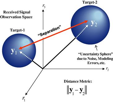
Figure 14.8 Illustration of the two-target ID problem. The goal of the joint transmitter/receiver design is to maximally separate the received signals in observation space, which in turn maximizes the probability of correct classification for the additive unimodal monotonic distributed noise case under fairly general conditions.
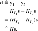
Significantly, ![]() and
and ![]() depend on the transmit signal s, as shown in (14.40). Consequently, it should be possible to select an s that maximizes the separation between
depend on the transmit signal s, as shown in (14.40). Consequently, it should be possible to select an s that maximizes the separation between ![]() and
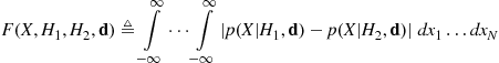
and ![]() , thereby maximizing the probability of correct classification under modest assumptions regarding the conditional probability density functions (PDFs) (e.g., unimodality), that is,
, thereby maximizing the probability of correct classification under modest assumptions regarding the conditional probability density functions (PDFs) (e.g., unimodality), that is,
![]() (14.41)
(14.41)
where
 (14.42)
and where
![]() (14.43)
(14.43)
Substituting (14.42) into (14.41) yields
![]() (14.44)
(14.44)
This is precisely of the form (14.10) and thus has a solution yielding maximum separation given by
![]() (14.45)
(14.45)
It is noted that (14.45) has an interesting interpretation: ![]() is that transmit input that maximally separates the target responses and is thus the maximum eigenfunction of the transfer kernel
is that transmit input that maximally separates the target responses and is thus the maximum eigenfunction of the transfer kernel ![]() formed by the difference between the target transfer matrices (i.e., (14.43)). Again if the composite target transfer matrix is stochastic,
formed by the difference between the target transfer matrices (i.e., (14.43)). Again if the composite target transfer matrix is stochastic, ![]() is replaced with its expected value
is replaced with its expected value ![]() in (14.45).
in (14.45).
Conditions for strict statistical optimality of the above optimization can be established by examining the properties of the conditional PDFs:
![]() (14.46)
(14.46)
For the case when the two conditional PDFs differ due to a shift in their means (generally multidimensional), an eminently reasonable assumption given the additive noise model of (14.40), the situation at hand can be illustrated as in Figure 14.9. We see that maximizing ![]() minimizes the overlap of the PDFs provided:
minimizes the overlap of the PDFs provided:
![]() (14.47)
(14.47)
where
 (14.48)
with
![]() (14.49)
(14.49)
Note that ![]() when
when ![]() . Clearly the class of multivariate Gaussian PDFs satisfies the above. Interestingly, even non-Gaussian PDFs can satisfy the above such as the class of unimodal distributions [23], and a broad class of elliptically contoured distributions [24]. This is in stark contrast to receiver optimization where generally the Gaussian assumption is required to ensure strict optimality [6].
. Clearly the class of multivariate Gaussian PDFs satisfies the above. Interestingly, even non-Gaussian PDFs can satisfy the above such as the class of unimodal distributions [23], and a broad class of elliptically contoured distributions [24]. This is in stark contrast to receiver optimization where generally the Gaussian assumption is required to ensure strict optimality [6].

Figure 14.9 Illustration of the impact of the separation metric d on the overlap of the conditional PDFs.
2.14.4.1 Application: two-target identification example
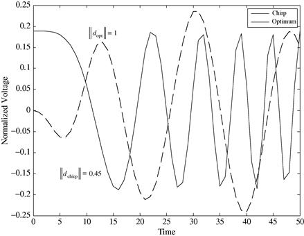
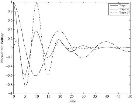
Let ![]() and
and ![]() denote the impulse responses of targets #1 and #2, respectively (Figure 14.10). Figure 14.11 shows two different (normalized) transmit waveforms—LFM and optimum (per (14.45))—along with their corresponding normalized separation norms of 0.45 and 1, respectively, which corresponds to 6.9 dB improvement in separation. To determine the relative probabilities of correct classification for the different transmit waveforms, one would first need to set the SNR level, which fixes the conditional PDF herein assumed to be circular Gaussian, and then to measure the amount of overlap to calculate the probability [6].
denote the impulse responses of targets #1 and #2, respectively (Figure 14.10). Figure 14.11 shows two different (normalized) transmit waveforms—LFM and optimum (per (14.45))—along with their corresponding normalized separation norms of 0.45 and 1, respectively, which corresponds to 6.9 dB improvement in separation. To determine the relative probabilities of correct classification for the different transmit waveforms, one would first need to set the SNR level, which fixes the conditional PDF herein assumed to be circular Gaussian, and then to measure the amount of overlap to calculate the probability [6].

An examination of Figure 14.12 reveals the mechanism by which enhanced separation is achieved. It shows the Fourier spectrum of ![]() , along with that of
, along with that of ![]() . Note that
. Note that ![]() places more energy in spectral regions where
places more energy in spectral regions where ![]() is large (i.e., spectral regions where the difference between targets is large, which is again an intuitively appealing result).
is large (i.e., spectral regions where the difference between targets is large, which is again an intuitively appealing result).
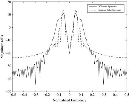
Figure 14.12 Comparison of the two-target difference spectrum and the optimum pulse spectrum. Note that the optimum pulse emphasizes parts of the spectrum where the two targets differ the most.
While pulse modulation was used to illustrate the optimum transmit design equations, we could theoretically have used any transmit DOF (e.g., polarization). The choice clearly depends on the application at hand.
2.14.4.2 Multi-target identification case
Given L targets in general, we wish to ensure that the L-target response spheres are maximally separated (an inverse sphere packing problem [25]). To accomplish this, we would like to jointly maximize the norms of the set of separations ![]() :
:
 (14.50)
Since, by definition, ![]() is given by
is given by
![]() (14.51)
(14.51)
Equation (14.50) can be rewritten as
 (14.52)
Since ![]() is the sum of positive semidefinite matrices, it shares this same property, and thus the optimum transmit input satisfies
is the sum of positive semidefinite matrices, it shares this same property, and thus the optimum transmit input satisfies
![]() (14.53)
(14.53)
2.14.4.3 Application: multitarget ID
Figure 14.13 depicts the impulse responses of three different targets, two of which are the same as in Section 2.14.4.1. Solving (14.52) and (14.53) yields an optimally separating waveform whose average separation defined by (14.50) is 1.0. This is compared with 0.47 for the LFM of Example 3.4, an improvement of 6.5 dB, which is slightly less than the previous two-target example. As expected, the optimum waveform significantly outperforms the unoptimized pulse waveform such as the LFM.
2.14.5 Constrained optimum transmit-receiver radar
Often there are a number of additional practical considerations (beyond finite norm) that may preclude transmitting the unconstrained optimum solutions developed so far. We will thus consider two cases of constrained optimization: linear and nonlinear—the latter is generally far more challenging and an area of active research.
2.14.5.1 Case 1: Linear constraints
Consider the linearly constrained version of the input (transmitter) optimization problem:
![]() (14.54)
(14.54)
![]() (14.55)
(14.55)
where ![]() . To avoid the overly constrained case, it is assumed that
. To avoid the overly constrained case, it is assumed that ![]() . For example, the rows of G could represent steering vectors associated with known interferers such as unwanted targets or clutter discretes to which we wish to apply transmit nulls.
. For example, the rows of G could represent steering vectors associated with known interferers such as unwanted targets or clutter discretes to which we wish to apply transmit nulls.
Equation (14.55) defines the feasible solution subspace for the constrained optimization problem. It is straightforward to verify that the projection operator
![]() (14.56)
(14.56)
projects any ![]() into the feasible subspace [26]. Thus, we can first apply the projection operator then perform an unconstrained subspace optimization to obtain the solution to (14.54) and (14.55), that is,
into the feasible subspace [26]. Thus, we can first apply the projection operator then perform an unconstrained subspace optimization to obtain the solution to (14.54) and (14.55), that is,
![]() (14.57)
(14.57)
From (14.53) it is readily apparent that the constrained optimum transmit input satisfies
![]() (14.58)
(14.58)
2.14.5.1.1 Application: pre-nulling on transmit
If there are known AOAs for which it is desired not to transmit (e.g., unwanted targets, clutter discrete, keep-out zones), it is possible to formulate a linearly constrained optimization accordingly.
Assume that there is a desired target at ![]() as well as two keep-out angles (normalized)
as well as two keep-out angles (normalized) ![]() and
and ![]() . The corresponding elements of the target transfer matrix
. The corresponding elements of the target transfer matrix ![]() , assuming an N-element ULA, are thus given by
, assuming an N-element ULA, are thus given by
![]() (14.59)
(14.59)
where ![]() denotes the (m,n)th element of the target transfer matrix.
denotes the (m,n)th element of the target transfer matrix.
The keep-out constraints have the form
 (14.60)
where
 (14.61)
Figure 14.14 shows the resulting constrained optimum transmit pattern for the case where ![]() . As expected a peak is placed in the desired target direction with nulls simultaneously placed in the keep-out directions.
. As expected a peak is placed in the desired target direction with nulls simultaneously placed in the keep-out directions.
2.14.5.2 Case 2: Nonlinear constraints
In practice other generally nonlinear constraints may arise. One family of such constraints relates to the admissibility of transmit waveforms, such as the class of constant modulus and stepped frequency waveforms [11], to name but a few.
For example, if it is desired to transmit a waveform that is nominally of the LFM type (or any other prescribed type) but that is allowed to modestly deviate to better match the channel characteristics, then the nonlinear constrained optimization has the form
![]() (14.62)
(14.62)
![]() (14.63)
(14.63)
The previous and similar problems cannot generally be solved in closed form. However, approximate methods can yield satisfactory results, and we will consider two that are based on very different approaches. These simpler methods could form the basis of more complex methods, such as seeding nonlinear search methods.
2.14.5.2.1 Relaxed projection approach
Figure 14.15 depicts the constrained optimization problem in (14.62) and (14.63). It shows the general situation in which the unconstrained optimum solution does not reside within the constrained (i.e., admissible) subspace ![]() . In this particular case, the admissible subspace is a convex set [27], defined as
. In this particular case, the admissible subspace is a convex set [27], defined as
![]() (14.64)
(14.64)
From Figure 14.15 it is also immediately evident that the admissible waveform closest (in a normed sense) to the unconstrained optimum ![]() lies on the surface of
lies on the surface of ![]() along the direction
along the direction ![]() , which is the unit norm vector that points from
, which is the unit norm vector that points from ![]() to
to ![]() , i.e.,
, i.e.,
![]() (14.65)
(14.65)
Thus, the constrained waveform that is closest in norm to ![]() is given by
is given by
![]() (14.66)
(14.66)
Note that if ![]() is allowed to relax to the point where
is allowed to relax to the point where ![]() , then
, then ![]() .
.
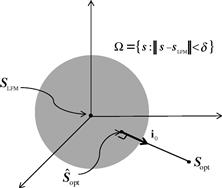
Figure 14.15 Illustration of a constrained optimization in which the signal should lie within a subspace (in this case convex) defined to be close to a prescribed transmit input (in this case an LFM waveform). The optimum relaxed projection is the point closest to the unconstrained optimum but still residing in the subspace.
2.14.5.2.2 Application: relaxed projection example
Here an LFM similarity constraint is imposed on the multipath interference problem considered previously. Specifically, in Figure 14.16, we plot the loss in SINR relative to the unconstrained long-pulse optimum solution previously obtained as a function of ![]() , which is varied between
, which is varied between ![]() . Note that for this example improvement generally monotonically increases with increasing
. Note that for this example improvement generally monotonically increases with increasing ![]() (except for a very small region near the origin) and that sizeable SINR improvements can be achieved for relatively modest values of the relaxation parameter. In other words, a waveform with LFM-like properties can be constructed that still achieves significant SINR performance gains relative to an unoptimized LFM.
(except for a very small region near the origin) and that sizeable SINR improvements can be achieved for relatively modest values of the relaxation parameter. In other words, a waveform with LFM-like properties can be constructed that still achieves significant SINR performance gains relative to an unoptimized LFM.
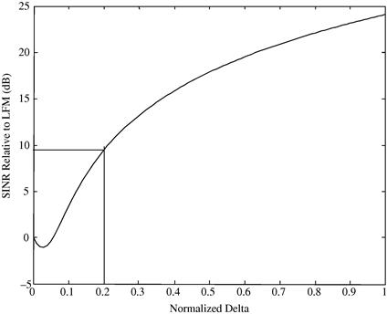
Figure 14.16 Illustration of the relaxed projection method for constrained optimization. The plot shows the SINR improvement relative to the unoptimized LFM waveform versus the normalized relaxation parameter ![]() . Note that for even a modest relaxation of 20% a nearly 10 dB gain in performance is achieved.
. Note that for even a modest relaxation of 20% a nearly 10 dB gain in performance is achieved.
Figure 14.17 shows the spectra of the unoptimized LFM along with the unconstrained optimum and the relaxed projection pulse with a 20% relaxation parameter. Note how the relaxed pulse is significantly closer to the original LFM spectrum yet still achieves nearly a 10 dB improvement in SINR relative to the LFM waveform.

2.14.5.2.3 Constant modulus and the method of stationary phase
As has become apparent from the previous examples, spectral shaping plays a key role in achieving matching gains. The stationary phase method has been applied to the problem of creating a nonlinear frequency modulated (NLFM) pulse (and thus constant modulus in the sense that the modulus of the baseband complex envelope is constant, i.e., ![]() ) with a prescribed magnitude spectrum [3,11].
) with a prescribed magnitude spectrum [3,11].
Specifically, under fairly general conditions [3,11] it is possible to relate instantaneous frequency ![]() of a NLFM waveform to time t [3,11]:
of a NLFM waveform to time t [3,11]:
 (14.67)
![]()
where ![]() is the magnitude spectrum of the optimum pulse. Here we have assumed a constant modulus for the NLFM waveform resulting in a integral that is simply proportional to time (see [3,11] for the more general nonconstant modulus case) as well as a finite and causal pulse.
is the magnitude spectrum of the optimum pulse. Here we have assumed a constant modulus for the NLFM waveform resulting in a integral that is simply proportional to time (see [3,11] for the more general nonconstant modulus case) as well as a finite and causal pulse.
Solving for ![]() as a function of t in (14.67) yields the frequency modulation that will result in a transmit pulse with a magnitude spectrum equal to
as a function of t in (14.67) yields the frequency modulation that will result in a transmit pulse with a magnitude spectrum equal to ![]() , to within numerical and other theoretical limitations [3,11].
, to within numerical and other theoretical limitations [3,11].
2.14.5.2.4 Application: NLFM to achieve constant modulus
Here we use the method of stationary phase to design a constant modulus NLFM pulse that matches the magnitude spectrum of the optimum pulse derived for the multipath interference problem previously considered.
Figure 14.18 shows the numerically obtained solution to (14.67) (i.e., ![]() versus t) along with the optimum pulse spectrum (long-pulse case). Note that as one would intuit, the frequency modulation dwells at frequencies where peaks in the optimum pulse spectrum occur and conversely note the regions in which the modulation speeds up to avoid frequencies where the optimum pulse spectrum has nulls or lower energy content.
versus t) along with the optimum pulse spectrum (long-pulse case). Note that as one would intuit, the frequency modulation dwells at frequencies where peaks in the optimum pulse spectrum occur and conversely note the regions in which the modulation speeds up to avoid frequencies where the optimum pulse spectrum has nulls or lower energy content.
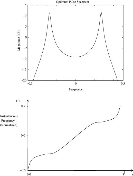
Figure 14.18 Illustration of the use of the method of stationary phase to create a constant modulus NLFM pulse whose spectral magnitude matches that of the optimum pulse. The NLFM pulse was able to achieve an output SINR that was within 6.0 dB of the optimum compared with a 24 dB loss using an LFM waveform of same energy and duration.
The constant modulus NLFM waveform so constructed was able to achieve an output SINR that was within 6.0 dB of optimum compared with a 24 dB loss using an LFM waveform of same energy and duration.
It is natural to ask if a NLFM waveform with the same spectral magnitude as the optimum pulse (but not necessarily the same phase) will enjoy some (if not all) of the matching gains. For the steady-state case (infinite time duration) this is indeed true, since from Parseval’s [3] theorem the output energy is related to only the spectral magnitudes (i.e., without their phases) of the input pulse and channel transfer function, that is,
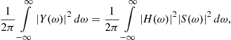 (14.68)
where ![]() denote the Fourier transforms of the channel output, channel impulse response, and input pulse, respectively. Note that the output energy in (14.68) depends on the spectral magnitude of the input pulse (steady-state)—not the phase. Thus, in theory an NLFM waveform that exactly matches the optimum pulse magnitude spectrum will achieve the same matching gains in the steady-state limit (infinite pulse duration) for all square integrable (finite norm) functions.
denote the Fourier transforms of the channel output, channel impulse response, and input pulse, respectively. Note that the output energy in (14.68) depends on the spectral magnitude of the input pulse (steady-state)—not the phase. Thus, in theory an NLFM waveform that exactly matches the optimum pulse magnitude spectrum will achieve the same matching gains in the steady-state limit (infinite pulse duration) for all square integrable (finite norm) functions.
2.14.6 Open issues and problems
Perhaps amongst the foremost challenges is the development of robust and effective adaptive methods that can accurately estimate the full dimensional transmit-receive channel in real-time and solve for the optimum transmit-receive configuration—no mean feat. A basic outline of methods that include traditional sample statistics methods, orthogonal MIMO waveform concepts for channel probing, and knowledge-aided (KA) methods for leveraging any and all prior and/or externally available channel information can be found in [22] (and references cited therein).
Even if real-time channel characterization methods can be developed, the issue of solving a generally constrained multidimensional transmit-receive waveform optimization problem remains. Here again it is desired to develop a set of efficient and reliable algorithms amenable to real-time implementation. Fortunately, steady advances in HPEC ensure that ever more increasing real-time compute power should be available.
2.14.7 Conclusions and future trends
In this chapter, the fundamental theory for joint optimization of the transmit and receive functions was developed from first principles and applied to the maximization of SINR, SCR, and correct classification for the target ID problem. Constrained optimization was introduced to address additional requirements that often arise in practice, such as the use of constant modulus waveforms to maximize transmitter efficiency. However, many theoretical and practical issues remain before the new field of adaptive transmit technology can be fully exploited.
As mentioned above, many challenges remain in realizing the full potential of joint transmit-receive optimization. Consequently, much of the current research trends in this area are focused on:
• Real-time methods for accurate multidimensional channel characterization.
• Robust and efficient algorithms for solving the generally constrained transmit-receive design equations.
• Leveraging of knowledge-aided (KA) methods such as those developed under the DARPA/AFRL KASSPER project [28,29].
• Combining other waveform diversity concepts with adaptive transmit-receive optimization to allow for enhanced multi-functionality.
Glossary
MIMO A system with multiple inputs and outputs. In radar it refers to multiple transmit and receive DoFs (usually multiple antennas for example)
SINR Signal-to-interference-plus-noise ratio. A measure of signal strength relative to all sources of interference (clutter, jamming, receiver noise, etc.)
Colored Noise A random (noise) process that has a non-identity matrix covariance matrix (usually involving non-zero off diagonal terms)
Whitening Filter The first stage in an optimum matched filter receiver when the additive noise has some correlation. The filter “whitens” the noise spectrum, which is then followed by a standard matched filter
Cauchy-Schwarz theorem In its simplest form, a theorem that states that the dot product of two vectors is maximum when they are co-linear
Multipath Electromagnetic propagation through a non-line-of-sight (NLOS) channel
FIR Filter Finite impulse response filter. A discrete time LTI tapped delay line filter
LFM Linear frequency modulation. A type of radar waveform whose instantaneous frequency varies linearly with time over a prescribed bandwidth
Radar Clutter Radar echo returns from objects other than the desired target(s). Ground reflections is the most common form of clutter
SCR Signal-to-clutter ratio. A relative measure of signal strength to clutter power
Signal Dependent Noise Interference whose statistics depend on the radar’s transmissions
Constant Modulus Refers to a class of waveforms whose complex envelope (modulation) has a constant modulus, i.e., ![]()
NLFM Nonlinear FM. A class of constant modulus waveform whose instantaneous frequency changes in a non-linear fashion
Acronyms
Acronyms that are commonly used in this chapter include the following:
AESA active electronically scanned array
CA-CFAR cell-averaging constant false alarm ratio
GMTI ground moving target indication
KASSPER knowledge-aided sensor signal processing and expert reasoning
LFM linear frequency modulation
PDF probability density function
PRF pulse repetition frequency
SINR signal-to-interference-plus-noise ratio
STAP space-time adaptive processing
Relevant Theory: Signal Processing Theory
See Vol. 1, Chapter 2 Continuous-Time Signals and Systems
See Vol. 1, Chapter 3 Discrete-Time Signals and Systems
See Vol. 1, Chapter 4 Random Signals and Stochastic Processes
See Vol. 1, Chapter 12 Adaptive Filters
References
1. Lawson JL, Uhlenbeck GE. Threshold signals. In: New York: McGraw-Hill; 1950; MIT Radiation Laboratory Series. vol. 24.
2. Guerci JR. Space-Time Adaptive Processing for Radar. Norwood, MA: Artech House; 2003.
3. Papoulis A. Signal Analysis. New York: McGraw-Hill; 1984.
4. Barton DK. Modern Radar System Analysis. Norwood, MA: Artech House; 1988.
5. Papoulis A. Circuits and Systems: A Modern Approach. New York: Holt, Rinehart and Winston; 1980.
6. Trees HLV. Detection, Estimation and Modulation Theory, Part I. New York: Wiley; 1968.
7. Horn RA, Johnson CR. Matrix Analysis. Cambridge (England), New York: Cambridge University Press; 1990.
8. Strang G. Introduction to Linear Algebra. Wellesley Cambridge Press 2003.
9. Pierre DA. Optimization Theory With Applications. Courier Dover Publications 1986.
10. Guerci JR, Pillai SU. Theory and application of optimum transmit-receive radar. In: The Record of the IEEE 2000 International Radar Conference. 2000;705–710.
11. Cook CE, Bernfeld M. Radar Signals. New York: Academic Press; 1967.
12. Richards MA. Fundamentals of Radar Signal Processing. McGraw-Hill 2005.
13. Lindenfeld MJ. Sparse frequency transmit-and-receive waveform design. IEEE Trans Aerosp Electron Syst. 2004;40:851–861.
14. Pillai SU, et al. Optimal transmit-receiver design in the presence of signal-dependent interference and channel noise. IEEE Trans Inform Theory. 2000;46:577–584.
15. Rabideau DJ. Closed loop multistage adaptive beamforming. In: Conference Record of the 33rd Asilomar Conference on Signals, Systems and Computers. 1999;98–102.
16. Van Trees HL, Detection E. Modulation Theory, Part II. New York: John Wiley and Sons; 1971.
17. Trees HLV. Detection, Estimation, and Modulation Theory: Radar-Sonar Signal Processing and Gaussian Signals in Noise. Krieger Publishing Co., Inc. 1992.
18. Pillai S, Burns C. Array Signal Processing. New York: Springer-Verlag; 1989.
19. Monzingo RA, Miller TW. Introduction to Adaptive Arrays. SciTech Publishing 2003.
20. Guerci J, Jaska E. ISAT—innovative space-based-radar antenna technology. In: IEEE International Symposium on Phased Array Systems and Technology. 2003;45–51.
21. R. Manasse, The Use of Pulse Coding to Discriminate Against Clutter, vol. AD0260230, Defense Technical Information Center (DTIC), June 7, 1961.
22. Guerci JR. Cognitive Radar: The Knowledge-Aided Fully Adaptive Approach. Norwood, MA: Artech House; 2010.
23. Ibragimov IA. On the composition of unimodal distributions. Theory Probab Appl. 1956;1:255.
24. Fang KT, Zhang YT. Generalized Multivariate Analysis. Beijing: Science Press; 1990.
25. Hsiang WY. On the sphere packing problem and the proof of Kepler’s conjecture. Int J Math. 1993;4:739–831.
26. Gander W, et al. A constrained eigenvalue problem. Linear Algebra Appl. 1989;114:815–839.
27. Youla DC, Webb H. Image restoration by the method of convex projections: Part 1 Theory. IEEE Trans Med Imag. 1982;1:81–94.
28. Gini F, Rangaswamy M, eds. Knowledge Based Radar Detection, Tracking and Classification Adaptive and Learning Systems for Signal Processing, Communications and Control Series. New York: Wiley-IEEE Press; 2008.
29. Guerci JR, Baranoski EJ. Knowledge-aided adaptive radar at DARPA: an overview. IEEE Signal Process Mag. 2006;23:41–50.