
SAR Interferometry and Tomography: Theory and Applications
Gianfranco Fornaro* and Vito Pascazio†, ‡, *Istituto per il Rilevamento Elettromagnetico Ambientale (IREA), Consiglio Nazionale delle Ricerche (CNR), Napoli, Italy, †Dipartimento di Ingegneria, Università degli Studi di Napoli Parthenope, Napoli, Italy, ‡Laboratorio Nazionale di Comunicazioni Multimediali, CNIT Complesso Universitario di Monte S. Angelo, Edificio Centri Comuni, Napoli, Italy, [email protected], [email protected], [email protected]
Abstract
Synthetic Aperture Radar (SAR) is among of the most used remote sensing systems for Earth observation and has wide application in security in both marine and terrestrial environments. The last decade has been a period of extraordinary development of SAR systems with an impressive growth in the number of launch and operational deployment of spaceborne SAR remote sensing systems. Enabling an extensive range of new applications is the advent of several very high resolution spaceborne SARs, such as TerraSAR-X/Tandem-X and the COSMO-SKYMED constellation. Very fine details of Earth surface are provided on a regular basis by data acquired and processed by those sensors. A significant contribution to the desire to field such systems has been the development of coherent processing techniques, in particular interferometry, that have dominated SAR applications since their first demonstration in the late 70s and early 80s. Evidence of the importance and versatility of radar interferometry is its application to such diverse area as the monitoring of volcanoes, earthquakes, landslides, ice sheet motion and anthropogenic sources such as ground pumping of water and oil. Development of innovative processing techniques, like permanent scatterer interferometry, polarimetric-interferometry and tomography have expanded the number of applications and data sets that can be successfully exploited. For example, permanent scatterer interferometry and tomography have revolutionized what can be done by SARs in urban environments. In this article we aim to provide a description of the some of the major developments in SAR interferometry and SAR tomography with particular emphasis on the digital signal processing aspects. We will illustrate SAR tomography using urban and infrastructures applications although it has other applications such as in forest and ice structure. Examples of applications of interferometry and tomography are provided to demonstrate the practical usefulness of the technological advances occurring on both the SAR system and data processing. With respect to other published tutorial on interferometry, we focus on the development of multibaseline/multipass coherent processing approach from a signal processing perspective with the aim to provide to readers a comprehensive description of the topics demanding to the reference bibliography deeper investigations.
Keywords
Synthetic Aperture Radars (SAR); Radar imaging; SAR Interferometry (InSAR); SAR Tomography (TomoSAR); Differential Interferometry (DinSAR); 3D-SAR imaging; 4D-SAR imaging
Acknowledgments
The Authors wish to thank the anonymous Reviewers for their comments which contributed to improve the quality of the paper, and Prof. Gilda Schirinzi, Prof. Alessandra Budillon, Prof. Giampaolo Ferraioli, and Dr. Fabio Baselice, of the Universitá di Napoli Parthenope, Italy, and Dr. Diego Reale of IREA-CNR, Napoli, Italy, for the valuable discussions about the main topics of the paper. Moreover, the Authors wish to thank Prof. Richard Bamler of DLR and Technical University of Munich, Germany, and Dr. Michael Eineider of DLR, Germany, and Dr. Alessandro Ferretti, of Telerilevamento Europa (TRE), Italy, for providing some of the images included in this paper. The Authors wish to thank also Prof. Fabrizio Lombardini of University of Pisa for providing the Capon results relevant to the San Paolo Stadium data set, and Dr. Nicola D’Agostino of the Istituto Nazionale di Geofisica e Vulcanologia for providing the GPS data used in Figure 20.25.
2.20.1 Introduction
During the 19th century, the theory of electromagnetic fields became a firmly established science: Maxwell’s equations accurately described the propagation of the fields, Marconi’s wireless experiments demonstrated the possibility of wireless communication at large distances. Nevertheless, even since that early time it was evident that electromagnetic waves could be not only used for communication but also to obtain information, or better to “sense” the environment and the objects without being in contact with them.
Remote sensing is today well established and intensively used for acquiring information about the Earth’s surface [1]: among the most used remote sensing systems, active microwave sensors and particularly Synthetic Aperture Radar (SAR) have gained an increasing interest from both a scientific and industrial viewpoint. This success is a consequence of the capability of the sensor to operate independently of an external illumination source (day and night) and practically in almost any meteorological condition.
2.20.1.1 Microwave high resolution imaging
Active sensors make use of radars, typically installed on spacecraft, or on aircraft, or even on ground. They transmit a coherent (i.e., well controlled at the level of a single oscillation) signal and record the echoes scattered back to the sensor from the observed area. Accordingly, they are independent from any external illumination sources: this peculiarity, together with the fact that they work at wavelength that are, differently from optical and infrared sensors, almost immune to the presence of clouds and fog, provide the system with the possibility to operate day and night and also in adverse weather conditions.
Modern SAR sensors transmit signals whose bandwidth is of the order of tens/hundreds MHz, thus leading to spatial resolution along the range (typically called across track direction) of the order of meters or fraction of meter.
For comparable optical aperture and antenna size, the spatial resolution along the flight track of images acquired by microwave sensors should be several order of magnitude worse than the optical images. This drawback is however overcome by the possibility to synthesize a very large antenna (of the order of few kilometers) by moving a much smaller real antenna along a straight trajectory corresponding to the platform flight track. This possibility, first postulated by Wiley [2] with the Doppler beam sharpening concept, is a direct consequence of the coherent nature of the system.
The operation of synthesizing a large antenna is today carried out typically off-line, after the downlink to a ground station, via a digital processing operation, usually referred to as SAR focusing operation, that, coherently combine on a 2D domain the echoes received from the radar at different positions. The obtained images are characterized by a resolution along the direction of array synthesis (typically referred to as along track direction) of the order of the length of the physical antenna dimension, independently from the wavelength and the height of the platform. Depending on the operative mode (scan, strip, and spot-mode) and on the fact that the platform can be disturbed during its motion by turbulences as in the airborne case, this operation can be in some cases more problematic.
SAR images are complex entities where the intensity basically measures the energy backscattered by the ground targets toward the sensor, which depends on the geometric (shape, roughness, and slope) and on physical (conductivity and permittivity) properties of the observed scene.
SAR sensors provide information about the observed scene complementary to that provided by optical systems. SAR images are nowadays used in many areas of interest: In glaciology they are used for glaciers monitoring and snow mapping, in agriculture for crop classification and soil moisture monitoring, in forestry for biomass estimation, etc. They are also used in environment monitoring for the detection of oil spills, flooding, as well as to monitor the urban growth or moving targets.
The technique that has opened probably the widest range of application is SAR Interferometry [3,4].
As in any electromagnetic coherent system the phase information is related to the travelled path, that is the distance target-sensor (range). Radar measurements therefore embed the information of distances with extreme high accuracy, on the order of wavelength fraction: due to the randomness of the scattering mechanism this information can be however extracted only as a relative measurement between different images. SAR Interferometry (InSAR) is a technique that, by exploiting at least two SAR images acquired from slightly different angles, allows retrieving the topography of the observed scene. A single SAR image provides measurement of measure the backscattering scene property only on a 2D domain, i.e., by performing a projection onto the plane containing the flight direction and the radar line of sight. Similarly to the human eyes system, height sensitivity can be achieved by combining two images of the same area acquired from two slightly different positions. The key principle of SAR interferometry is the use of the phase difference between SAR images for the accurate measurement of the distances of a target from two sensors displaced in location in order to create a parallax.
The two images can be acquired simultaneously if two antenna are present at the same time on the platform (single-pass interferometry) or through different passes of the same antenna (repeat-pass interferometry). In the latter case changes of the scene backscattering properties and variations of the phase delay contribution from the atmosphere may strongly impair the accuracy of the results. The accuracy of the topography estimation depends on the component orthogonal to the line of sight of the antenna vector separation commonly referred to as (spatial) baseline: for this reason this technique is also referred to as across-track interferometry.
As an alternative to topographic mapping, when the two antennas are present on the same platform and are separated along the flight direction, they acquire images repeated with a revisit of a few milliseconds. This is the case of the along-track interferometry which allows monitoring fast movements of targets on the ground. Applications concern for example the estimations of ocean currents or moving detection and velocity estimation [5].
An interesting extension of across and along-track InSAR is the Differential SAR Interferometry (DInSAR): by exploiting phase difference of images acquired at times (epochs), separated typically by some days, it allows accurately monitoring slow displacements over the epoch sequence. Differential interferometric data can be acquired by radar observations separated in time either from a single radar on one platform (e.g., ERS-1, JERS-1, ENIVSAT, TerraSAR-X) or from multiple radars on different platforms provided the radar have similar radar operating a viewing parameters (e.g., Cosmo Skymed constellation). Since the precision of radar in estimating distance is in the order of fraction of wavelength, DInSAR can estimate movements with sub-centimetric accuracy using L-, C-, or X-Band radars.
Major applications of this technique regard the natural hazard and security area. Besides, by exploiting archives of past images multipass techniques are also extremely useful to provide a past monitoring.
Interferometry applications have dramatically increased the use of microwave remote sensing for the environment monitoring: This is also testified by the growing interest of the major international space agencies in the development and launch of spaceborne SAR sensors satellites. The twin satellites ERS-1 and ERS-2 [6] of the European Space Agency (ESA), operative since 1992 and 1996, respectively, each one with a revisiting time of 35 days each, were characterized by the possibility to acquire a pairs of tandem images, i.e., interferometric images separated by only one day. ERS sensors from nineties to the first decade of 2000 were the very first systems used for the operative demonstration and routinely application of interferometry. Their acquisitions have been deeply exploited for years to develop most of the interferometric processing algorithm currently used and to demonstrate the potentials of the application of SAR Interferometry in several natural risk areas. Recently, the Italian Cosmo Skymed [7] and German TerraSAR-X [8] missions improved the quality of SAR product by providing images with spatial resolution up to one meter. Together with its twin satellite TanDEM-X, TerraSAR-X is going to provide the most accurate Digital Elevation Model (DEM), i.e., the topography, of the Earth on a global scale with a relative accuracy of 2 m for slope lower than 20° and 4 m for higher slopes with a spatial grid of 12 m. From the other side, the Italian COSMO-Skymed mission [7] is, worldwide, the unique constellation of more than two SAR sensors exploited also for civilian applications. It is composed of four medium-size satellites, each one equipped with an X-band high-resolution SAR system, allowing acquiring images on the same area every 4 days on average, thus both reducing the effects of decorrelation and allowing a more frequent imaging which is useful for interferometric application to cases of emergency.
Polarimetry [9–16] and Polarimetric SAR interferometry [17,18] and are techniques that use multi-polarization channels to extract further information on the scattering mechanism. Polarimetric information allows separating different scattering mechanisms. Whereas SAR polarimetry is a technique that use single antenna data, Polarimetric SAR interferometry use data acquired by two antennas. The former has a wide use in the field of classification, the latter allows generating interferograms corresponding to different scattering mechanisms and has an area of application in the field of forest height retrieval and biomass estimation.
The advances in the SAR hardware has allowed to reach very high imaging resolutions at microwaves on the order of a meter and has in parallel stimulated the development of advanced processing techniques able to extract from the data the highest possible information content.
One of the most important and recent innovations in SAR processing is associated with the extension of the imaging process form a 2D domain to a multi-dimensional domain. The so-called SAR Tomography has been among the first examples giving to SAR the ability of reconstructing images of the backscattering property of the scene also along the direction (elevation) orthogonal to the two classical dimension (azimuth and range). The key aspect of this technique is the possibility to synthesize, similarly to the flight direction (azimuth) an array also along the “height” direction to sharpen and steer the beam in such a way to measure the backscattering characteristics of the scene along the elevation direction and hence to generate full 3D images.
SAR Tomography allows vertically profiling (3D imaging) the backscattering to detect targets which interfere in the same pixel of a single SAR image and even monitoring, with the extension of the imaging properties to the time direction (4D Imaging), their individual deformation. Beside the application to a distributed scenario such as forest where the scattering is distributed along the height, the tomographic technique also provide significant advances in the application to the imaging and monitoring of in areas characterized by an high density of scatterers, such as urban areas, opening the possibility to achieve dense imaging and monitoring of single buildings and individual structures from the space, for the first time comparable to what obtainable with in situ systems like laser scanner [19,20].
Polarimetric SAR tomography [21–24] takes benefits of both polarimetry and tomography: by accessing the multibaseline information on different polarization channels, it allows retrieving scattering profiles along the elevation direction associated with different scattering mechanisms such as single bounce, double bounce and volume scattering. This work concentrates on the development of SAR interferometry (including multipass Differential SAR Interferometry) and Tomography for 3D reconstruction and target deformation monitoring.
2.20.2 Basics concepts in SAR imaging and SAR interferometry
2.20.2.1 High resolution image formation
Among the several parameter characterizing an image, resolution plays certainly a major role. In the radar case the resolution along the range coordinate depends on the system bandwidth [25,26]. Large bandwidths are obtained, with simplified (i.e., low peak power) hardware, by transmitting long duration linear frequency modulated (chirp) pulses which are, after echo reception, compressed (typically on the ground) via correlation techniques: this operation is commonly referred to as range pulse-compression or range focusing (see Figure 20.1).

The transmitted chirp pulse has the following expression:
![]() (20.1)
(20.1)
wherein rect[![]() ] is the window function,
] is the window function, ![]() is the pulse duration, and
is the pulse duration, and ![]() is the Chirp rate
is the Chirp rate ![]() . The correlation of the response of a target at range r with the transmitted pulse replica provides the expression of the range impulse response function (IRF), also known as range Point Spread Function (PRF):
. The correlation of the response of a target at range r with the transmitted pulse replica provides the expression of the range impulse response function (IRF), also known as range Point Spread Function (PRF):
![]() (20.2)
(20.2)
with c being the light-speed and ![]() the bandwidth of the transmitted pulse. The (3 dB) range resolution is numerically given by [27]
the bandwidth of the transmitted pulse. The (3 dB) range resolution is numerically given by [27]
![]() (20.3)
(20.3)
Such a resolution value is also referred to as slant range resolution to highlight that it refers to the line-of-sight (LOS) direction. Scaling factors derived by standard trigonometry should be applied to achieve the resolution along the main scene direction, for instance along the direction corresponding to the projection of range onto the local cartographic reference system usually referred to as ground range resolution:
![]() (20.4)
(20.4)
where ![]() is the so-called incident angle, defined as the angle between the radar LOS and the local normal to the surface at the point of the reflection on the ground (see Figure 20.2), and
is the so-called incident angle, defined as the angle between the radar LOS and the local normal to the surface at the point of the reflection on the ground (see Figure 20.2), and ![]() is the terrain slope. The ground range resolution is, of course, coarser than the slant range resolution.
is the terrain slope. The ground range resolution is, of course, coarser than the slant range resolution.

Figure 20.2 SAR range resolution. ![]() is the slant range resolution,
is the slant range resolution, ![]() is the ground range resolution,
is the ground range resolution, ![]() is the look angle,
is the look angle, ![]() is the incidence angle, and
is the incidence angle, and ![]() is the local terrain slope. In absence of topography
is the local terrain slope. In absence of topography ![]() , it results that
, it results that ![]() .
.
Note that in the absence of terrain slope, the incidence angle is equal to the angle ![]() (known as look angle and defined with respect to the nadir direction) only when the Earth curvature can be neglected, i.e., as in the case of airborne sensors operating at low altitude.
(known as look angle and defined with respect to the nadir direction) only when the Earth curvature can be neglected, i.e., as in the case of airborne sensors operating at low altitude.
In case of flat ground and if the SAR antenna beamwidth in the range direction is not too big, as usually occur for instance for new generation X-band SAR sensors, the ground resolution is almost constant along the footprint. Differently, in case of non-flat ground, as shown in Figure 20.3, the ground resolution can change significantly, as effect of topography, giving rise to the well known effects of foreshortening, layover, and shadowing. Under conditions of foreshortening different resolution cells can contain contribution of very different, in terms of dimension, ground areas (see Figure 20.3b). Layover is beyond the limit case just described: in this case, points more distant in the ground can appear closer to the SAR radar sensor, and are mapped erroneously in the SAR image (see Figure 20.3c). Such effect is very common in mountainous areas with steep slopes, and in urban areas [4]. The shadowing effect occurs when ground area are masked by reliefs, as in Figure 20.3d. In this last case, a slant range resolution cell does not map any ground area (the ground area BC in Figure 20.3d is not seen from the SAR antenna). The above presented distortion effects makes that SAR images of mountain and urban areas can look very different from optical images, as an effect of geometrical distortions.
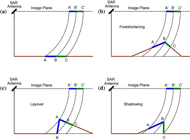
Figure 20.3 SAR distortion effects: (a) normal conditions, (b) foreshortening, (c) layover, and (d) shadowing.
In the azimuth direction the focusing operation is necessary to synthesize a long antenna with higher resolution capabilities, that is for achieving the beam sharpening.
With reference to Figure 20.4 where the system imaging geometry represented in the flight direction, the system “senses” the scene by transmitting pulses at regular time instants, regulated by the pulse repetition frequency. The echoes collected in each position may be coherently processed in such a way to synthesize (digitally) an antenna whose dimension is equal to the footprint (X) of the real antenna [25,28]:
![]() (20.5)
(20.5)
where ![]() is the wavelength, L is the azimuth length of the real antenna, and r is the range of the target (range). Note that
is the wavelength, L is the azimuth length of the real antenna, and r is the range of the target (range). Note that ![]() is the angular aperture of the real SAR antenna in the azimuth direction. The final resolution of the image, provided by the synthetic antenna is [25]:
is the angular aperture of the real SAR antenna in the azimuth direction. The final resolution of the image, provided by the synthetic antenna is [25]:
![]() (20.6)
(20.6)
where the resolution gain factor 2 in the first equality is associated with the capability of the array to transmit and receive the radiation from each position of the real antenna during the synthetic antenna formation.
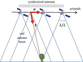
Figure 20.4 System geometry in the azimuth direction. The movement of the platform allows to synthesize a larger antenna thus achieving a sharpening of the beam of the real antenna.
The time interval in which the scatterer is illuminated is referred to as integration time: for a standard operating mode, as that illustrated in Figure 20.4 (referred to as stripmap mode), it is trivially given by the ratio between the real antenna footprint and the platform velocity (v).
A dual approach used for the computation of the azimuth resolution of the focused image is provided by the so called Doppler analysis which states that when either transmitters or receiver are subject to a uniform motion, the received radiation is subject to a frequency shift (called Doppler shift) equal ![]() , with
, with ![]() being the velocity vector (in our case of the platform) and
being the velocity vector (in our case of the platform) and ![]() being the versor of the receiving radiation (in our case the direction locating the scatterer from the platform). It is therefore clear that, during the integration interval, the echo from the target sweeps an interval from
being the versor of the receiving radiation (in our case the direction locating the scatterer from the platform). It is therefore clear that, during the integration interval, the echo from the target sweeps an interval from ![]() to
to ![]() , which corresponds to a Doppler frequency interval from
, which corresponds to a Doppler frequency interval from ![]() to
to ![]() . Accordingly, the Doppler bandwidth amounts to:
. Accordingly, the Doppler bandwidth amounts to:
![]() (20.7)
(20.7)
Such a bandwidth is able to provide pulses with time duration equals L/(2v), which corresponds a spatial extent of about L/2. Unfortunately, the relative motion between the sensor and the target introduces also linear (phase) distortions as well as motion through resolution cell. Therefore, to provide short duration pulses the phase distortions affecting the available bandwidth must be compensated at the azimuth focusing level with the use of filters which are intrinsically 2D and also space variant only (for rectilinear tracks) with the range. The SAR focusing topic is out of the scope of this work, readers can refer to [25,28].
2.20.2.2 Operational modes
The classical operational mode of a SAR system considers the antenna pointing with a fixed offset from the flight direction, non-necessary orthogonal (i.e., broadside) pointing: this is referred to as Stripmap mode to highlight the fact that the scene is illuminated along a strip. The stripmap imaging mode geometry is depicted in Figures 20.4 and 20.5a.

In this way the integration time for forming the image of a target is, as discussed in the previous section, limited by the ratio between the real antenna azimuth footprint dimension and the platform velocity. This poses a limitation on the maximum achievable resolution. Another limitation of this imaging mode is associated with the coverage of the imaged strip in the slant range direction, which is in this case provided by the ground range extent of the real antenna footprint [25]. Slant range coverage and imaging resolution can be traded-off by operating a beam steering during the acquisition. Beside the classical stripmap mode, the two most known operational mode are spotlight and scan mode.
In the Spotlight mode the antenna beam is steered backward with respect to the antenna flight direction in such a way to collect data from a fixed area on ground on a longer (compared with the classical stripmap mode) flight segment [26,29,30]. The spotlight imaging mode geometry is depicted in Figure 20.5b.
In particular with respect to the stripmap mode (Figure 20.5) where the beam orientation is fixed, in the spotlight mode what is fixed is the illuminated area: this spotlight configuration is usually referred to as staring spotlight mode. A configuration that allow obtaining illumination interval and hence resolutions between the stripmap and staring spotlight mode is the so called sliding spotlight in which the angular beam steering rate is reduced in such a way to allow the footprint to slide on the ground [31,32]. With respect to the staring spotlight, the resolution loss is compensated by an increase of the azimuth coverage.
A mode complementary to the spotlight is the ScanSAR mode [33] whose geometry is shown in Figure 20.6. In this case the antenna is steered in the range direction to increase the range coverage. During the aperture synthesis in azimuth, the beam is regularly steered in range to sweep among a fixed number (typically 2–4) of adjacent range subswaths. The sweep mechanism is carried out in such a way to avoid gaps along the azimuth direction over the subswaths, i.e., to avoid the presence of areas which are not illuminated in the azimuth direction. The data collected in an illumination sub-interval for a generic subswath is called burst. In the stripmap case each target is imaged from the whole antenna beam and therefore the radiometric accuracy is preserved, that is homogenous area are imaged in a (average) constant backscattering level. In the ScanSAR case, as the target is seen only from a, or from a few small portions of the azimuth beam during the burst acquisition, not only we have a reduction of the azimuth resolution (this is the price for the increase in the range cover), but also different areas can be seen by different portions of the azimuth antenna beam. The latter effect produces radiometric losses seen as stripes along the azimuth (scalloping): homogenous area are imaged in a variable backscattering level. A mitigation of the scalloping problem is achieved by the adopting a TOPS (literally reverse of SPOT) acquisition mode [34]. In this case, in addition to the range steering, a steering in azimuth, with a forward rotation (i.e., opposite to that of the SPOT mode), is carried out to allow the azimuth beam to run forward, faster that the platform, in such a way that almost all scatterers in azimuth are imaged by the highest possible beam portion.
The azimuth resolution for the different modes can be evaluated by referring to the Doppler bandwidth, evaluated in (20.7), which can be written as a product of the Doppler rate ![]() and the integration time
and the integration time ![]() :
:
![]() (20.8)
(20.8)
Equation (20.8) follows directly from the fact that the signal collected along the azimuth direction (slow time) is with a good approximation a linear frequency modulated pulse; the associated Doppler rate ![]() equals:
equals:
![]() (20.9)
(20.9)
In the Stripmap case the integration time is fixed by the real antenna beamwidth:
![]() (20.10)
(20.10)
By substituting Eqs. (20.10) and (20.9) in Eq. (20.8), Eq. (20.7) is obtained. In the Scansar and Spotlight cases, due to the range or azimuth antenna sweep, the integration time is fixed to a value which is lower and higher than the limit in (20.10), respectively, in order to select the wanted azimuth resolution.
It is important to point out also that, while in the Stripmap case the spectral properties of the received signal are time invariant along the azimuth, in the case of Scansar and Spotlight acquisition, due to the antenna steering, the spectral properties show an azimuth space variance. For instance, in the spotlight mode, and particularly in the sliding spotlight configuration, due to the difference between the platform and footprint velocity, the angular view of the system to the scene is azimuth dependent and accordingly, the received Doppler bandwidth is progressively translated from positive to negative frequencies. All these aspects must be accounted during post processing, such as for instance image resampling and/or image filtering as in the case of SAR interferometry [35].
2.20.3 SAR interferometry
SAR image is a 2D complex signal, resulting from the coherent processing of raw data acquired from the synthetic antenna [26]. The amplitude of the SAR images represents the reflectivity of the ground area under view while the phase of the SAR images is randomly distributed [26,36]. In addition to electromagnetic scattering properties of the targets, the latter embeds also very important geometrical measurements.
Such information can be extracted exploiting two [37–39] (or more than two [40–42] SAR complex images in the framework of SAR interferometry. In particular, the term SAR Interferometry (InSAR) is referred to all methods that employ at least two complex SAR images, exploiting mainly their phases, in order to derive more information about a ground scene respect to the information provided by a single SAR image. The additional information is provided when at least one among the key acquisition parameters of the SAR system is different from acquisition to acquisition.
There exist two possible main configurations of SAR Interferometry: across track interferometry [38] and along track interferometry [43]. In the across track configuration, two (or more) SAR sensors fly on two parallel flight lines and look at the ground from slightly different look angles. In the along-track configuration, two (or more) sensors fly on the same path, looking the scene from the same position but with a very small temporal gap. The across track InSAR configuration allows recovering the height profile of the ground area under observation, while the InSAR along track configuration is mainly used for measurement of fast displacements such as ocean currents [44] and for moving target detection and velocity estimation [45,46].
In all interferometric processing the starting point are the SAR complex images, that can be obtained by means of a two dimensional (2D) processing of the raw data acquired from the SAR sensors [47]. The SAR complex images z(x,r) are representative of the reflectivity of the ground scene, in the sense that they are 2D discrete complex signals of the azimuth (x) and range (r) coordinates, where each sample (an image pixel) embeds the mean reflectivity characteristics of a sampling cell of the ground scene.
2.20.3.1 Across-track SAR interferometry for measuring the surface topography
The regular and controlled oscillation of coherent radiation used in SAR systems allows determining with high accuracy the variations of the propagation distance: such a basic property is the key principle of interferometric techniques.
A single SAR image provides measurement about the backscattering scene property along two directions: The target range (i.e., the distance of the target from the illumination track) and the position of the target along the track (the azimuth direction). Hence, no information is provided on the angle under which the target is imaged (look angle). Knowledge of the latter information completes the set of coordinates in a cylindrical reference system with the axis coincident with the track, thus allowing a full localization of the scatterers in 3D and therefore an estimation of topography.
Similar to the mechanism used in human visual system for the determination of the depth, SAR interferometry is a technique that exploits the parallax in the view of the scene to allows extending the capability of a single SAR system to the reconstruction of the scene elevation profile: as SAR is sensitive to distance whereas the visual system is sensitive to angles, the mechanism is indeed slightly different.
Figure 20.7 shows the geometry of a basic (two-antenna) interferometric acquisition in the plane orthogonal to the flight track: it is clear that by measuring the range of the target with a single (master) SAR system (say the blue line) it is not possible to uniquely localize the position of the scatterer because at the same range would be located all of the points distributed on a equi-range curve (the blue1 one) in the elevation beam (dash line).

By using a second (slave) antenna that images the scene from a different look angle the system is able to measure also the range from a second location [48]: there is then only one point (the intersection of the two equi-range, i.e., blue and red lines in Figure 20.7) that obey to the distance measurements pair. The larger the separation between the two antennas, the sharper the crossing and hence the higher the height accuracy. As in the visual system the 3D sensitivity is given by the difference in the location of the object in the two images at the different eyes [37], the accuracy of the stereometric system in Figure 20.7 is related to the variation of the distance of the target from one to the other antenna (range difference). To provide sufficient accuracy in such a range variation, SAR interferometry uses the phase difference between the two SAR images: the path difference is hence measured to an accuracy which is a fraction of the wavelength (centimeters at microwaves).
Specifically, the terms that plays the key role in the determination of the height is the path difference ![]() . In particular, at large distances it can be shown that the (variation of) the path difference (with respect to a reference point for instance located on a plane) is [37,39]:
. In particular, at large distances it can be shown that the (variation of) the path difference (with respect to a reference point for instance located on a plane) is [37,39]:
![]() (20.11)
(20.11)
where (see Figure 20.7) ![]() is the variation of the look angle between the master and slave antenna,
is the variation of the look angle between the master and slave antenna, ![]() is the orthogonal baseline component, that is the component orthogonal to the (master) line of sight of the vector (baseline) connecting the two satellites, and
is the orthogonal baseline component, that is the component orthogonal to the (master) line of sight of the vector (baseline) connecting the two satellites, and ![]() is the incidence angle, that is the angle between the vertical direction related to the target and the direction of the incoming radiation (line of sight). It is however important to note that Eq. (20.11) represent a simplification of the true scenario which is useful to understand the key principles of across-track interferometry. In the reality, the height is referred to a geographic or cartographic reference system and determined by measuring
is the incidence angle, that is the angle between the vertical direction related to the target and the direction of the incoming radiation (line of sight). It is however important to note that Eq. (20.11) represent a simplification of the true scenario which is useful to understand the key principles of across-track interferometry. In the reality, the height is referred to a geographic or cartographic reference system and determined by measuring ![]() and by knowing the orbital state vectors [49].
and by knowing the orbital state vectors [49].
In SAR interferometry the path difference is measured to accuracy of the order of the wavelength by using the phase difference signal:
![]() (20.12)
(20.12)
For application to topographic mapping the two interferometric images can, or better should be acquired at the same time by two antennas on the same platform (bistatic system). This is because changes in the scattering properties, as well as differences in the propagation phase delay through the atmosphere strongly impact the quality of the retrieved DEM. In the case of the Shuttle Radar Topography Mission (SRTM) in 2001 an extensible boom 60 m long was mounted on-board the Shuttle to separate the slave from the master antenna available in the fuselage [50]. The German TanDEM-X mission of 2010 is instead the first example of a bistatic system composed by two twin satellites (TerrSAR-X and Tandem-X) orbiting in a close (500 m one behind the other) formation [51].
2.20.3.2 Statistical characterization of across-track SAR interferometric signals
As mentioned before, an Across Track SAR interferometric (InSAR) system is used to reconstruct earth topography, providing high precision Digital Elevation Model (DEM) of Earth surface. The geometry of an InSAR system has already been shown in Figure 20.7, where two SAR systems look at the scene from two slightly different tracks. As already introduced, the distance b between the two SAR tracks is called baseline, its component orthogonal to the look direction ![]() is the orthogonal baseline, while its component parallel to the look direction (to the slant range)
is the orthogonal baseline, while its component parallel to the look direction (to the slant range) ![]() is the parallel baseline.
is the parallel baseline.
In order to understand how an InSAR system works, consider the distance ![]() between the first SAR antenna
between the first SAR antenna ![]() and a point target T on the ground, and the distance
and a point target T on the ground, and the distance ![]() between the second SAR antenna
between the second SAR antenna ![]() and the same point target T, as shown in Figure 20.7, while
and the same point target T, as shown in Figure 20.7, while ![]() and
and ![]() denote the angles at which the two antennas look at the point target on the ground (slightly different from each other).
denote the angles at which the two antennas look at the point target on the ground (slightly different from each other).
Consider now the two complex (envelope of the) images ![]() and
and ![]() obtained processing raw data collected by the two SAR sensors, where (n,m) are the discrete coordinates corresponding to the continuous azimuth and range coordinates (x,r). Such images can be considered as random processes whose expression is [52]:
obtained processing raw data collected by the two SAR sensors, where (n,m) are the discrete coordinates corresponding to the continuous azimuth and range coordinates (x,r). Such images can be considered as random processes whose expression is [52]:
![]() (20.13)
(20.13)
where ![]() is the complex envelope of the (deterministic) ground reflectivity function (which, in first approximation, can been assumed to be constant with the antenna position k
is the complex envelope of the (deterministic) ground reflectivity function (which, in first approximation, can been assumed to be constant with the antenna position k ![]() 1, 2, since, as commented above, the view angles change only slightly from one position to another),
1, 2, since, as commented above, the view angles change only slightly from one position to another), ![]() are phase factors related to the different propagation paths between the two antenna positions and the point target, and
are phase factors related to the different propagation paths between the two antenna positions and the point target, and
![]() (20.14)
(20.14)
is the random process representing the multiplicative speckle noise at the kth antenna, typical of any coherent system, which is commonly assumed to be a complex Gaussian correlated process with zero mean and unit variance [53]. Of course, ![]() are also random processes.
are also random processes.
As result of the SAR signal model given by (20.13) and (20.14), the phase of a SAR image pixel (n,m) is given by three main contributions:
• a first term ![]() , representing the phase shift induced by the scattering mechanism; it is deterministic, and it is the same for the two antennas;
, representing the phase shift induced by the scattering mechanism; it is deterministic, and it is the same for the two antennas;
• a second term ![]() , representing the phase shift due to the different propagation; it is deterministic, and it is depends on the antenna;
, representing the phase shift due to the different propagation; it is deterministic, and it is depends on the antenna;
• a third term ![]() , induced by the coherent nature of the SAR processing; it is
, induced by the coherent nature of the SAR processing; it is ![]() , and it is depends on the antenna.
, and it is depends on the antenna.
Other phase terms related to geometrical uncertainties, to random propagation effects, or to the changes of the scattering mechanism between the two SAR image acquisitions (for instance, due to the time delay between the two acquisitions) can be also present in Eq. (20.13).
After a processing called image registration which aims to locate the response of a target in the azimuth range pixel in the two images same pixel [37,54], the two SAR images ![]() and
and ![]() are used to build the so-called multi-look SAR interferogram:
are used to build the so-called multi-look SAR interferogram:
 (20.15)
where arg(![]() denotes the principal value of the phase,
denotes the principal value of the phase, ![]() is the number of looks [26], and the explicit dependence on (n,m) has been understood (the same will be made in the following). Equation (20.15) represents, for homogeneous targets, the Maximum Likelihood Estimator (MLE) of the interferometric phase [39]. In the following, we will consider the single look case, with
is the number of looks [26], and the explicit dependence on (n,m) has been understood (the same will be made in the following). Equation (20.15) represents, for homogeneous targets, the Maximum Likelihood Estimator (MLE) of the interferometric phase [39]. In the following, we will consider the single look case, with ![]() .
.
From (20.12) and (20.13), it is easy to show that the interferometric phases are related to the observed scene height profile through the well known mapping [3,53]:
![]() (20.16)
(20.16)
where ![]() denotes the modulo
denotes the modulo ![]() operation and
operation and
![]() (20.17)
(20.17)
is the decorrelation phase noise related to the phase differences of the speckle. In Eq. (20.16) it has been assumed, as commented before, that the scattering phase term ![]() , is constant in the two SAR images, so their differences vanishes.
, is constant in the two SAR images, so their differences vanishes.
The problem to be solved in across track InSAR consists of estimating the height values ![]() , starting from the measured (then, noisy) wrapped phases
, starting from the measured (then, noisy) wrapped phases ![]() . Such problem is worldwide known as phase-unwrapping problem, as it amounts to find the unwrapped phase
. Such problem is worldwide known as phase-unwrapping problem, as it amounts to find the unwrapped phase ![]() (not constrained to belong to the interval [0,2
(not constrained to belong to the interval [0,2![]() )) corresponding to the measured wrapped phase
)) corresponding to the measured wrapped phase ![]() (constrained to belong to the interval [0,2
(constrained to belong to the interval [0,2![]() )) [55]:
)) [55]:
![]() (20.18)
(20.18)
The unwrapped phase will be proportional to an estimate of the height h, according to the model given by Eq. (20.12):
![]() (20.19)
(20.19)
Once that the phase unwrapping problem (20.18) has been solved, an estimate of the height profile can be obtained from Eq. (20.19).
Equation (20.19) shows how much sensitive is the unwrapped phase with the height. Considering a fixed geometry for the satellite (or airplane) carrying the SAR antennas (![]() and
and ![]() are fixed), it is easy to understand that the larger the orthogonal baseline and the larger the frequency, the more sensitive is the SAR interferometer. In other words, if we want to measure the height profile h, it could seem more convenient to use a larger baseline and a higher frequency, because for a given variance of the phase noise, the corresponding height variance (inaccuracy) decreases (see Eq. (20.19)). However, an increase of the baseline value may contributes to decorrelate the two speckle phase contributions (
are fixed), it is easy to understand that the larger the orthogonal baseline and the larger the frequency, the more sensitive is the SAR interferometer. In other words, if we want to measure the height profile h, it could seem more convenient to use a larger baseline and a higher frequency, because for a given variance of the phase noise, the corresponding height variance (inaccuracy) decreases (see Eq. (20.19)). However, an increase of the baseline value may contributes to decorrelate the two speckle phase contributions (![]() and
and ![]() , thus increasing the interferometric phase noise (geometrical or spatial decorrelation) [56,57]. For a distributed scattering the correlation between the two speckle contributions decreases linearly with the increase of the baseline [37,39], for a point scatterer the decorrelation disappear because such targets are not affected by speckle. The difference between such two scattering mechanisms influences also the multipass interferometric processing chains (see Section 2.20.4). In any case an increase in the baseline impact also the degree of complexity of the phase unwrapping step described in the following sections.
, thus increasing the interferometric phase noise (geometrical or spatial decorrelation) [56,57]. For a distributed scattering the correlation between the two speckle contributions decreases linearly with the increase of the baseline [37,39], for a point scatterer the decorrelation disappear because such targets are not affected by speckle. The difference between such two scattering mechanisms influences also the multipass interferometric processing chains (see Section 2.20.4). In any case an increase in the baseline impact also the degree of complexity of the phase unwrapping step described in the following sections.
Before describing in the following sub-section part the several methods that have been proposed in the scientific literature to solve the phase unwrapping problem [42,58–63], it is important to describe the random nature of the SAR complex signal and of the SAR phase terms.
Consider the random terms ![]() given by (20.14), representing the multiplicative speckle noise present in the SAR complex signals
given by (20.14), representing the multiplicative speckle noise present in the SAR complex signals ![]() given by (20.13). Such random terms can be modeled as zero mean, mutually correlated Gaussian complex variables with unit variance, which assume uncorrelated values in adjacent pixels, and have real and imaginary parts mutually uncorrelated [52]. By understanding the dependence on range and azimuth discrete co-ordinates n and m, for the sake of simplicity of notation, we can consider the vector:
given by (20.13). Such random terms can be modeled as zero mean, mutually correlated Gaussian complex variables with unit variance, which assume uncorrelated values in adjacent pixels, and have real and imaginary parts mutually uncorrelated [52]. By understanding the dependence on range and azimuth discrete co-ordinates n and m, for the sake of simplicity of notation, we can consider the vector:
![]() (20.20)
(20.20)
whose (real valued) elements ![]() and
and ![]() , with k
, with k ![]() 1,2, denoting the cosine and sine components of the speckle signal
1,2, denoting the cosine and sine components of the speckle signal ![]() , are zero mean Gaussian random variables. The assumed statistical model implies that [52]:
, are zero mean Gaussian random variables. The assumed statistical model implies that [52]:
Note that the ![]() independence is true if the speckle band-pass spectrum is Hermitian respect to the central frequency, assumption which can be considered always satisfied since the speckle vector
independence is true if the speckle band-pass spectrum is Hermitian respect to the central frequency, assumption which can be considered always satisfied since the speckle vector ![]() is related to the complex envelope of a modulated real signal [64]. Moreover, from the assumption (b), it stems that
is related to the complex envelope of a modulated real signal [64]. Moreover, from the assumption (b), it stems that ![]() .
.
In these assumptions, the probability density function of the vector ![]() is given by [65]:
is given by [65]:
![]() (20.21)
(20.21)
where ![]() , and C is the covariance matrix given by:
, and C is the covariance matrix given by:
 (20.22)
where ![]() is the correlation coefficient of
is the correlation coefficient of ![]() and
and ![]() , which by virtue of assumption (b) assume the same value of the correlation coefficient of
, which by virtue of assumption (b) assume the same value of the correlation coefficient of ![]() and
and ![]() , given by:
, given by:
 (20.23)
where ![]() denotes expectation. Note that in Eq. (20.23) the terms present at the denominator are equal to one, as they represent the unit variance of the considered processes, so that their explicit presence should not be necessary. Nonetheless, we use such definition, as it is valid also in the case of not-normalized processes.
denotes expectation. Note that in Eq. (20.23) the terms present at the denominator are equal to one, as they represent the unit variance of the considered processes, so that their explicit presence should not be necessary. Nonetheless, we use such definition, as it is valid also in the case of not-normalized processes.
We note that, according to the assumptions (a) and (b), ![]() given by (20.23) is equal to the interferometric coherence usually employed in InSAR systems [57], defined starting from complex signals [3]:
given by (20.23) is equal to the interferometric coherence usually employed in InSAR systems [57], defined starting from complex signals [3]:
 (20.24)
Note that first result of Eq. (20.24)![]() implies that the coherence
implies that the coherence ![]() of the (complex) speckle noise is real valued, due to the above assumptions (a) and (b). Note also that the module of the coherence
of the (complex) speckle noise is real valued, due to the above assumptions (a) and (b). Note also that the module of the coherence ![]() of the complex received signals
of the complex received signals ![]() and
and ![]() is, in module, equal to the coherence
is, in module, equal to the coherence ![]() of the (complex) speckle noise.
of the (complex) speckle noise.
Starting from Eq. (20.21), it is possible to derive, by a change of variable from Cartesian to polar (from ![]() to
to ![]() , and following integration with respect to
, and following integration with respect to ![]() and
and ![]() , the pdf of the single-look speckle phase difference
, the pdf of the single-look speckle phase difference ![]() [53]:
[53]:
 (20.25)
where the dependence of phase difference ![]() and
and ![]() on (n,m) has been, as before, understood.
on (n,m) has been, as before, understood.
The coherence coefficient ![]() is influenced by all factors that cause differences between the two complex speckle images
is influenced by all factors that cause differences between the two complex speckle images ![]() and
and ![]() . The larger these differences, the smaller the coherence coefficient’s value. A coherence reduction can be induced by actual physical changes occurring between the acquisition times of the two data sets (temporal decorrelation) and/or by changes of the ground reflectivity when it is seen from different angles (spatial decorrelation) [57]. Note that also the coherence is a function of the ground coordinate pair (n,m), so that it may change across the image.
. The larger these differences, the smaller the coherence coefficient’s value. A coherence reduction can be induced by actual physical changes occurring between the acquisition times of the two data sets (temporal decorrelation) and/or by changes of the ground reflectivity when it is seen from different angles (spatial decorrelation) [57]. Note that also the coherence is a function of the ground coordinate pair (n,m), so that it may change across the image.
The plot of the speckle phase difference pdf (20.25) for different values of the coherence coefficient is given in Figure 20.8. It has to be noted that the pdf become less picked by reducing the coherence value. The smaller the coherence value, the larger the variance of the speckle phase noise.
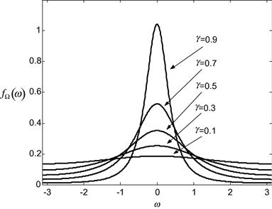
Figure 20.8 Interferometric phase pdf plotted for different coherence values (0.01, 0.1, 0.25, 0.5, 0.7, and 0.9).
The joint pdf ![]() of the interferometric phases can be obtained from the joint pdf of the speckle noise phase
of the interferometric phases can be obtained from the joint pdf of the speckle noise phase ![]() given by Eq. (20.25) and plotted in Figure 20.8, exploiting the random variable transformation given by Eq. (20.16), which leads to:
given by Eq. (20.25) and plotted in Figure 20.8, exploiting the random variable transformation given by Eq. (20.16), which leads to:
![]() (20.26)
(20.26)
where the dependence of phase difference ![]() , and
, and ![]() on (n,m) has been again understood. The pdf’s (20.26) have the same shape of pdf of Eq. (20.25), but they are centered on the value
on (n,m) has been again understood. The pdf’s (20.26) have the same shape of pdf of Eq. (20.25), but they are centered on the value ![]() h.
h.
Such pdf family, that as it can be noted is parametrized by the height h, will be used as starting point of some of the phase unwrapping methods described in the following section.
The pdf (20.26) of the interferometric phase is strongly influenced by the coherence. Such parameter can be written as the product of four main contributions [3,39,57]:
![]() (20.27)
(20.27)
where ![]() represents the influence of thermal noise in the receiver,
represents the influence of thermal noise in the receiver, ![]() represents the decorrelation effects due to the different SAR view acquisition angles, depending upon the spatial baseline,
represents the decorrelation effects due to the different SAR view acquisition angles, depending upon the spatial baseline, ![]() represents the decorrelation effects due to volume scattering mechanisms, and
represents the decorrelation effects due to volume scattering mechanisms, and ![]() represents the so called temporal decorrelation effects [3,4].
represents the so called temporal decorrelation effects [3,4].
The first factor in Eq. (20.27) can be computed starting from the circular Gaussian and independent nature of thermal noise and is given by:
![]() (20.28)
(20.28)
where ![]() and
and ![]() are the signal to noise ratio on the two receiving SAR interferometric antennas [4,53,57].
are the signal to noise ratio on the two receiving SAR interferometric antennas [4,53,57].
The second factor in Eq. (20.27) is the so-called geometric coherence, also referred to as angular or baseline coherence; it is present for all scattering situations, it depends on the system parameters and on the overall observation geometry, including the different SAR view acquisition angles, and depending upon the spatial baseline.
Geometric coherence values can be easily computed, in case of flat terrain, and for a white scattering process, leading to [3]:
 (20.29)
where ![]() is the orthogonal baseline and
is the orthogonal baseline and ![]() is the orthogonal critical baseline given by:
is the orthogonal critical baseline given by:
![]() (20.30)
(20.30)
where all symbols in Eq. (20.30) have been previously introduced.
Geometric decorrelation effects, for flat terrain geometry, can be explained also from the so-called spectral shift effect [55]. This interpretation allows also to derive a filtering strategy of the interferometric channels aimed at mitigating such decorrelation. Such proper processing is also called “common band filtering” [55,66], because requires to process, to maximize the geometric coherence value, the common (overlapped) part of the spectrum of the two interferometric signals. The larger the baseline, the larger the terrain slope, the less the common part of the two spectra, and the larger the decorrelation effects. For a non-flat topography the approach in [67] can be adopted. For the ERS and ASAR-ENVISAT sensors, the critical baseline is of about 1100 m for ![]() , while for the last generations high resolution systems such as COSMO-Skymed and TerraSAR-X, this value is significantly enlarged. Therefore, for these new generation sensors, thanks to fact that the distribution of the baseline values is bounded by an “orbital tubes” significantly smaller than the critical baseline, such common band filtering is typically not required.
, while for the last generations high resolution systems such as COSMO-Skymed and TerraSAR-X, this value is significantly enlarged. Therefore, for these new generation sensors, thanks to fact that the distribution of the baseline values is bounded by an “orbital tubes” significantly smaller than the critical baseline, such common band filtering is typically not required.
Similar effects can be induced also in the azimuth direction by the presence of variations of the azimuth antenna pointing [67]. This effect can be critical in some acquisition modes where antenna steering is present, such as in ScanSAR and Spotlight modes. Also in this case, the larger the acquisition geometric diversity, the less the spectra overlapping, and the larger the decorrelation effects.
The third factor in Eq. (20.27)![]() , is the volume coherence, it is due to volume scattering, and it is the effect induced by the scattering layer to increase the size projected range cell, and consequently, to decrease the correlation distance. As in the case of
, is the volume coherence, it is due to volume scattering, and it is the effect induced by the scattering layer to increase the size projected range cell, and consequently, to decrease the correlation distance. As in the case of ![]() , it is dependent on the spatial baseline.
, it is dependent on the spatial baseline.
The last factor in Eq. (20.27)![]() represents the so called temporal decorrelation [57] due to the instability of scattering mechanisms in the two different acquisition times, as the structure of the scatterer can change in the meantime between the two acquisitions. Such effect can be very important when the two SAR images are acquired at distance of several days or months in the case of vegetated or agricultural areas, or in presence of different climatic conditions.
represents the so called temporal decorrelation [57] due to the instability of scattering mechanisms in the two different acquisition times, as the structure of the scatterer can change in the meantime between the two acquisitions. Such effect can be very important when the two SAR images are acquired at distance of several days or months in the case of vegetated or agricultural areas, or in presence of different climatic conditions.
2.20.3.3 The differential SAR interferometry technique for measuring displacements
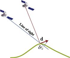
Differential Interferometry (DInSAR) is a particular configuration of SAR interferometry. The reference geometry is the same of the classical InSAR case, but the target on the ground is allowed to move, displacing of say ![]() , between the two successive passes (see Figure 20.9).
, between the two successive passes (see Figure 20.9).
In the following, for sake of simplicity, we indicate deterministic and stochastic terms all with non-capital symbols: the nature is specified whenever ambiguous. In this case, the interferometric phase is composed by three main factors:
![]() (20.31)
(20.31)
where ![]() is the measured range variation that, in the far field observation approximation, is equal to the component of the displacement along the line of sight,
is the measured range variation that, in the far field observation approximation, is equal to the component of the displacement along the line of sight, ![]() is the phase contribution corresponding to the target height as in Eq. (20.12),
is the phase contribution corresponding to the target height as in Eq. (20.12), ![]() is a stochastic term associated with the variation, between the two passes, of the wave propagation delay through the atmosphere,
is a stochastic term associated with the variation, between the two passes, of the wave propagation delay through the atmosphere, ![]() is the phase noise which in this case includes also the temporal decorrelation effects in addition to the decorrelation noise due to the speckle (
is the phase noise which in this case includes also the temporal decorrelation effects in addition to the decorrelation noise due to the speckle (![]() in Section 2.20.3.2). In the cases in which the topographic contribution is limited, that is if the baseline is negligible and/or an external DEM is available to compute and cancel out
in Section 2.20.3.2). In the cases in which the topographic contribution is limited, that is if the baseline is negligible and/or an external DEM is available to compute and cancel out ![]() from Eq. (20.31), and in the case of a predominance of the deformation component and/or limited effects of atmosphere, displacements can be measured to accuracy which are on the order of the wavelength. By using this classical two passes DInSAR configuration in the past Scientists have been able to capture the surface deformation field generated by major earthquakes, or highlight deformation associated with volcanic activities.
from Eq. (20.31), and in the case of a predominance of the deformation component and/or limited effects of atmosphere, displacements can be measured to accuracy which are on the order of the wavelength. By using this classical two passes DInSAR configuration in the past Scientists have been able to capture the surface deformation field generated by major earthquakes, or highlight deformation associated with volcanic activities.
The idea of mapping ground deformation via the interference of signals acquired by SAR systems was demonstrated for airborne systems in [43] and for the very first time using real data from the European Remote Sensing Satellite (ERS) in keystone experiments by [68], for ice-stream velocity measures in Antarctica, and by [69] for the co-seismic deformation field generated by the Landers earthquake (CA-USA). The Landers result received cover of Nature (vol. 364, 8 July 1993, Issue No. 6433) with a title “The image of an Earthquake” that translates the importance of the achievements and of the DInSAR technology with reference to application to seismic and to geo-hazards in general.
Today, with the availability of many SAR sensors with interferometric capabilities orbiting around the Earth, co-seismic, i.e., before and after main seismic events (see Figure 20.10), DInSAR data are almost analyzed routinely by scientists to study the displacements induced by known and unknown geological faults that are the causes of catastrophic events all over the world.

Figure 20.10 Co-seismic interferogram of the Bam earthquake obtained by a combination of Envisat Advanced Synthetic Aperture Radar (ASAR) Wide Swath Mode (WSM) image with an Image Mode (IM) image.Polimi/Poliba.
An example of measurement of DInSAR co-seismic displacement is reported to provide an idea of the powerfulness of this technology with reference to the 6.6 Mw Iran earthquake in 2003 that stroke the city of Bam. The image Figure 20.10, shows the co-seismic interferogram obtained by interferometric combination of the SCANSAR (Wide Swath Mode) acquisition of September 24th, 2003 and the STRIPMAP (Image Mode) acquisition of December 3rd, 2003: each color-cycle correspond to 1.55 cm in the line of sight. The coherence of the data and therefore the quality of the interferogram is very high due to the arid nature of the region: each color-cycle correspond to 2.8 cm displacement in the line of sight.
A key factor in such application is associated with the revisiting time. The retired satellites ERS-1, ERS-2, and ENVISAT of the Europen Space Agency have been the satellites on which repeat pass interferometry has been experimented for the very first time. These satellites were characterized in the normal operational situation by a strip width of approximately 100 Km EW and a revisiting time (i.e., the time necessary to repeat approximately the same orbit) of 35 days. The revisiting time poses a limitation to the minimum number of days necessary to generate an interferogram. The new generation of sensors operating at slightly lower orbits with respect to ERS and ENVISAT, such as TerraSAR-X and Tandem-X allows reducing the revisiting time to 11 days. The Italian COSMO-SkyMed (CSK) constellation is a constellation formed by four SAR satellites that acquires data for interferometric use, regardless of the specific satellite. This peculiarity allows CSK to provide the highest maximum revisit rate of an area of interest, that is one acquisition every 4 days (on average) for the whole constellation, instead of one acquisition every 16 days for a single satellite. CSK and TerraSAR-X provide spatial resolution (between ![]() and
and ![]() one order of magnitude better than the previous available C-Band satellite SAR data.
one order of magnitude better than the previous available C-Band satellite SAR data.
These systems operates in X-band and are characterized by higher spatial resolution with respect to the past ESA C-Band satellites; the counterpart of these advantages are however the reduced swath coverage which in the classical stripmap imaging mode reduces to 40 Km in the EW direction. An example of co-seismic interferogram obtained with a 8 days temporal baseline form COSMO-Skymed data is discussed in the following. On 6 April, 2009 the MW 6.3 L’Aquila earthquake occurred in the Central Apennines (Italy) causing extensive damage to the town of L’Aquila and killing 300 inhabitants. The event epicenter was located few kilometers southwest of the town of L’Aquila, the main shock nucleated at a depth of ![]() 9 km, was preceded by a preseismic sequence with the largest shock having a ML 4 magnitude, and was followed by a vigorous aftershock sequence. In Figure 20.11 it is shown the interferogram evaluated by the CSK pair of April 4th and April 12th: the activated fault is located NW-SE emerging to the right of the dense fringes area: each color-cycle correspond to 1.55 cm in the line of sight.
9 km, was preceded by a preseismic sequence with the largest shock having a ML 4 magnitude, and was followed by a vigorous aftershock sequence. In Figure 20.11 it is shown the interferogram evaluated by the CSK pair of April 4th and April 12th: the activated fault is located NW-SE emerging to the right of the dense fringes area: each color-cycle correspond to 1.55 cm in the line of sight.

Figure 20.11 Co-seismic interferogram of 6 April 2009 6.0 Mw l’Aquila earthquake in Italy. COSMO-Skymed acquisitions of 4 April 2009 and 12 April 2009.
Since then, many experiments showed the potentiality of the technique in detecting deformation phenomena not only associated with earthquakes [70] but also in volcanic areas [71,72] and of glaciers [73].
However, in order to fully exploit the potentiality of the SAR technology in order to measure deformation with a centimetric/millimetric accuracy two or few images are typically not sufficient. At such accuracy level the presence of the atmospheric component and additional disturbing contributions such as orbital inaccuracies cannot be in fact neglected. For sake of simplicity we indicate still with ![]() the differential interferometric phase obtained after the subtraction of the contribution associated with the DEM (differential interferogram). We have therefore:
the differential interferometric phase obtained after the subtraction of the contribution associated with the DEM (differential interferogram). We have therefore:
![]() (20.32)
(20.32)
where ![]() is associated with orbital inaccuracies which affect the computation of the phase contribution associated with the topography (baseline error): as for Eq. (20.31), the noise term is associated with the noise contributions such as decorrelation of the response not only due to variation of the speckle contribution due to the angular imaging diversity (spatial baseline decorrelation), but also to changes of the backscattering response over the time (temporal decorrelation). Availability of on board GPS systems allows significantly mitigating the effects of orbital errors; for airborne systems which are subject to trajectory deviations due to turbulence the GPS must be integrated with accurate inertial navigation systems. Due to the DEM subtraction
is associated with orbital inaccuracies which affect the computation of the phase contribution associated with the topography (baseline error): as for Eq. (20.31), the noise term is associated with the noise contributions such as decorrelation of the response not only due to variation of the speckle contribution due to the angular imaging diversity (spatial baseline decorrelation), but also to changes of the backscattering response over the time (temporal decorrelation). Availability of on board GPS systems allows significantly mitigating the effects of orbital errors; for airborne systems which are subject to trajectory deviations due to turbulence the GPS must be integrated with accurate inertial navigation systems. Due to the DEM subtraction ![]() is now the residual target height, i.e., the height of the target with respect to the reference DEM. Accordingly, to have the possibility to achieve measurement of small deformation components, use of accurate external DEM as well as small baseline separations, is mandatory. In any case the atmospheric component plays a major role because it causes the presence of errors which are spatially correlated and therefore may be mixed with possible deformations.
is now the residual target height, i.e., the height of the target with respect to the reference DEM. Accordingly, to have the possibility to achieve measurement of small deformation components, use of accurate external DEM as well as small baseline separations, is mandatory. In any case the atmospheric component plays a major role because it causes the presence of errors which are spatially correlated and therefore may be mixed with possible deformations.
The atmospheric contribution is typically separated in two components: a turbulent component which is associated with the air inhomogeneity and that causes a spatial variation of the Atmospheric Phase Delay (APD) and a stratified component which is associated with the vertical stratification of the atmosphere. Both these terms occur in the lower part of the atmosphere, the troposphere, whereas contribution in the upper part of the atmosphere mainly show contributions which are very low spatial variable and can be misinterpreted as orbital inaccuracies. The former is commonly referred to as wet component and is dependent on the relative humidity, the latter, also referred to as hydrostatic or improperly as dry component, is responsible of a contribution which is highly correlated with the topography and therefore almost negligible on quasi flat areas. A model that describes the statistical behavior of the turbulent component is due to Kolmogorov. In this case the turbulence is assumed spatially stationary and isotropic. The refractivity index, i.e., the excess in parts per million of the reflectivity index with respect to the vacuum, that provided the increase in the path difference due to the crossing of the atmosphere can be modeled in terms of the variogram, i.e., the variance of the difference of the refractivity contributions between two points. For separations below the order of a kilometer, the variance of the difference of the refractivity between two points small and decreasing with a power of 2/3 of the distance. A more thoughtful characterization and analysis of the tropospheric contribution can be found in [74].
The temporal correlation of the atmosphere is however typically low: this means that APD contributions over different epochs can be averaged together to diminish it contribution on the path difference. Therefore to measure small (up to millimeter per year) displacements and to handle the problem of monitoring at high resolution ground scatterers, techniques based on the use of several images acquired over the same scene have been developed. In fact, by exploiting a higher dimensional acquisition space, the “phase firms” of the different components such as DEM error, displacement, and APD can be deterministically or stochastically characterized and estimated directly from the received data. This topic is treated in more details in Section 2.20.5.
2.20.3.4 Phase unwrapping
Unwrapping aims at reconstructing an unrestricted (absolute2) signal starting from a measured wrapped signal version restricted a reference interval. In the case of interferometry, the phase is intrinsically wrapped in the (![]() ) interval being extracted from complex values. Accordingly, we have:
) interval being extracted from complex values. Accordingly, we have:
![]() (20.33)
(20.33)
where ![]() and
and ![]() are the restricted (wrapped) and unrestricted (absolute) phase. Phase unwrapping is a step necessary to reconstruct a phase signal
are the restricted (wrapped) and unrestricted (absolute) phase. Phase unwrapping is a step necessary to reconstruct a phase signal ![]() which is an estimate of
which is an estimate of ![]() .
.
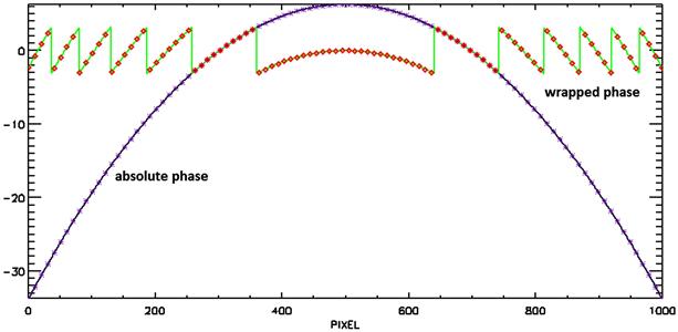
Figure 20.12 reports an example in a 1D case: phase unwrapping aims to estimate the absolute phase (shown in blue) starting from the measured restricted phase (shown in red).
It should also be noted that the term “absolute” phase in the interferometric context is typically used to refer to the phase corresponding to ![]() which has been corrected by an offset to account for the correct number of global cycles which are lost due to the wrapping operator and for the timing errors. In SAR interferometry such an offset is commonly evaluated after phase unwrapping by using one or more reference points with a known topography.
which has been corrected by an offset to account for the correct number of global cycles which are lost due to the wrapping operator and for the timing errors. In SAR interferometry such an offset is commonly evaluated after phase unwrapping by using one or more reference points with a known topography.
The problem of unwrapping is ambiguous as it admits in principle infinitely many solutions (the wrapped phase can be itself a possible absolute phase), and a reasonable solution can be obtained by imposing a certain degree of continuity: the absolute phase in Figure 20.12 is, among all possible absolute phase functions corresponding to the measured wrapped phase, the continuous one. Unfortunately, in real cases, in addition to the noise, the problem is further complicated by the presence of a finite sampling rate, see the measured red diamond samples in Figure 20.12 and the absolute black star samples corresponding to the absolute phase. Moreover, the actual solution could be locally not continuous.
In the following, some popular approaches to solve the phase unwrapping problem and to recover the height profile of the ground scene will be described.
2.20.3.4.1 Residue cut algorithms for PhU
Residue cut [75], also known as branch-cut algorithms have been a workhorse for the PhU for many years prior to the advent of more effective solutions based on Least Square and optimizations based on Linear Programming algorithms. The starting point of this approach is the estimation of the absolute phase variations along arcs ![]() wrapped phase variation
wrapped phase variation ![]() . In particular it results that
. In particular it results that
![]() (20.34)
(20.34)
where ![]() and where the first equality is taken as the definition of
and where the first equality is taken as the definition of ![]() that is of wrapped variation of the wrapped phase. Equation (20.34) states that, by wrapping the variation from sample to sample of the measured wrapped phase an estimate of the absolute phase variations can be retrieved provided that the latter is limited to the restriction interval, i.e., within the (
that is of wrapped variation of the wrapped phase. Equation (20.34) states that, by wrapping the variation from sample to sample of the measured wrapped phase an estimate of the absolute phase variations can be retrieved provided that the latter is limited to the restriction interval, i.e., within the (![]() ) interval.
) interval.
Following the stage of estimation of the absolute phase differences, an integration step of the estimated variations must be implemented to pass from ![]() to
to ![]() . Possible errors on a phase variation estimate, either due to an intrinsic variation of the absolute phase or to a missing wrapping jump due to the noise, propagates in all the subsequent samples during the integration process.
. Possible errors on a phase variation estimate, either due to an intrinsic variation of the absolute phase or to a missing wrapping jump due to the noise, propagates in all the subsequent samples during the integration process.
A way to control such errors is by measuring redundant variations: in the 1D case this is only possible if we measure the variations over non adjacent samples: this operation is however critical because of the higher probability to variations of the absolute phase larger than ![]() , thus impacting the validity of the approximation in Eq. (20.34). Fortunately, the 2D case allows having higher redundancy degree of even limiting the measurement of spatial variations over adjacent samples [76].
, thus impacting the validity of the approximation in Eq. (20.34). Fortunately, the 2D case allows having higher redundancy degree of even limiting the measurement of spatial variations over adjacent samples [76].
The basic idea of the residue cut algorithm is to follow elementary closed circuits defined on the set of image pixel and check for the presence of inconsistencies in the estimate of the absolute phase variation.
Following the stage of estimation of the absolute phase differences, the algorithm proceeds with the integration of the estimated variations but carries out a consistency check on the loops. By referring to Figure 20.13, we refer for simplicity to two elementary loops: the triangular shape of the circuits is a choice that is typically carried out when the phase unwrapping has to be carried out on a sparse grid. Assuming for instance an anticlockwise direction of the loops, it is clear that if the estimates of the true phase variation are correct, i.e., corresponding to the absolute phase we have:
![]() (20.35)
(20.35)
If, however, due to the wrapping operator in (20.34), at least one of the estimate is affected by errors, say ![]() for which we have that
for which we have that ![]() then the closed loops on the left in Eq. (20.35) do not sum up to zero:
then the closed loops on the left in Eq. (20.35) do not sum up to zero:
![]() (20.36)
(20.36)
In this situation, it is the loops are said to be affected by residues. It is clear that due to a choice of the loop orientation, residues appear always in pair. The line connecting the two residues, which are supposed to be located at the center of the loops, is referred to as cut and intersects the wrong absolute phase estimate: this phase variation is eliminated during the final integration patch covering all pixels.
2.20.3.4.2 Least squares and Green’s solution to PhU problem
We refer, for sake of simplicity, to a regular 2D grid (see Figure 20.14): it is possible to measure the horizontal ![]() (i,j) and vertical
(i,j) and vertical ![]() (i,j) variations between adjacent samples, leading to the measurement from the wrapped phase values of a 2D field
(i,j) variations between adjacent samples, leading to the measurement from the wrapped phase values of a 2D field ![]() , with
, with ![]() and
and ![]() , that represents an estimate of the gradient of the absolute phase.
, that represents an estimate of the gradient of the absolute phase.
Figure 20.14 Representation of the phase and phase variations on elementary closed loops for the phase unwrapping on a regular 2D grid.
As already explained in the previous section, the variation field should be zero curl, ![]() . Obviously, due to the 2
. Obviously, due to the 2![]() (multiple) errors that affect the variation field
(multiple) errors that affect the variation field ![]() , this condition is not always satisfied and therefore the result of the process of integration of the spatial variations to retrieve the unwrapped phase is dependent on the specific path. Instead of using circulation over elementary square paths to locate the presence of vortex (residues) and to trace cuts between opposite residues to avoid the integration path crossing areas over which summation over closed path is not zero, Least Squares and Green’s algorithm try to find a solution that carries out a global integration in such a way to mitigate the error propagation.
, this condition is not always satisfied and therefore the result of the process of integration of the spatial variations to retrieve the unwrapped phase is dependent on the specific path. Instead of using circulation over elementary square paths to locate the presence of vortex (residues) and to trace cuts between opposite residues to avoid the integration path crossing areas over which summation over closed path is not zero, Least Squares and Green’s algorithm try to find a solution that carries out a global integration in such a way to mitigate the error propagation.
Il particular the Least Squares approach looks for ![]() such that
such that ![]() is the “closest” (in some norm) to
is the “closest” (in some norm) to ![]() ; more specifically:
; more specifically:
![]() (20.37)
(20.37)
with typically ![]() . The least square solution
. The least square solution ![]() can be easily achieved by solving the Poisson equation [62,77]:
can be easily achieved by solving the Poisson equation [62,77]:
![]() (20.38)
(20.38)
for any ![]() internal to the domain of interest (say S), with the following boundary condition:
internal to the domain of interest (say S), with the following boundary condition:
![]() (20.39)
(20.39)
for any ![]() on the boundary (say C),
on the boundary (say C), ![]() being the normal unit vector on the boundary curve.
being the normal unit vector on the boundary curve.
An effective iterative implementation on a regular 2D grid can be achieved by iterating on each (internal) pixel the following equation:
![]() (20.40)
(20.40)
assuming left and right values of the unknown to be corresponding to the current and previous iteration, respectively. The iterative solution of (20.40) is appealing because it can be extended also to a sparse 2D grid via the use of triangulations. Iterative algorithms might be however time demanding depending on the size of the processed image: a more time-effective solution for a regular 2D grid is provided by frequency domain analysis. In particular, by using the Green’s function formulation it can be shown that the solution to (20.38) and (20.39) on a surface S with boundary C can be explicitly written as:
 (20.41)
wherein ![]() is approximated (in the discrete space case) with the variations measured from the wrapped data
is approximated (in the discrete space case) with the variations measured from the wrapped data ![]() and where g(r) is the free-space Green solution of the Laplace equation, i.e., :
and where g(r) is the free-space Green solution of the Laplace equation, i.e., :
![]() (20.42)
(20.42)
that is
![]() (20.43)
(20.43)
The solution in (20.41) is attractive because it allows to investigate analytically the spreading of errors related to the errors related to the substitution of the true gradient with the measured gradient, i.e., ![]() [61].
[61].
The Green solution requires, on the other hand, the knowledge of the true phase on the border, this problem can be solved by adopting an iterative scheme in which starting from ![]() is evaluated in all the points, including the boundary C. In the case of sparse grid of measurements where the boundary may be characterized by multiple curves, it is preferable to use the FD approximation to the differential equation.
is evaluated in all the points, including the boundary C. In the case of sparse grid of measurements where the boundary may be characterized by multiple curves, it is preferable to use the FD approximation to the differential equation.
2.20.3.4.3 Minimum cost flow solution to PhU problem
In both methods, FD approximation and Green, the solution do not honour the data, in the sense that ![]() is a multiple of 2
is a multiple of 2![]() because the Least Square solution intrinsically diffuse possible error in u over different pixels to achieve a global square minimum. Methods like the Minimum Discontinuity (MD) [78] and Minimum Cost Flow (MCF) allow “honouring” the data, by directly search in a discrete space the 2
because the Least Square solution intrinsically diffuse possible error in u over different pixels to achieve a global square minimum. Methods like the Minimum Discontinuity (MD) [78] and Minimum Cost Flow (MCF) allow “honouring” the data, by directly search in a discrete space the 2![]() multiple correction. The MD approach seeks for the 2
multiple correction. The MD approach seeks for the 2![]() k field that provides
k field that provides ![]() , with
, with ![]() collecting all the measured wrapped phase on the selected (full or sparse) grid, showing the minimum discontinuity between adjacent points. The MCF algorithm [60,79], operates in a similar way by seeking for the field of integers
collecting all the measured wrapped phase on the selected (full or sparse) grid, showing the minimum discontinuity between adjacent points. The MCF algorithm [60,79], operates in a similar way by seeking for the field of integers ![]() of correction to
of correction to ![]() (with minimum norm) such that the corrected variation field on a network defined over the set of available pixel is characterized by a null rotational component, i.e., it solves the problem:
(with minimum norm) such that the corrected variation field on a network defined over the set of available pixel is characterized by a null rotational component, i.e., it solves the problem:
 (20.44)
where ![]() is the (typically weighted) LP norm.
is the (typically weighted) LP norm.
The case ![]() is chosen for the capability to limit the number of points in which the correction is carried out, and at the same time allows using very efficient Linear Programming solvers [60].
is chosen for the capability to limit the number of points in which the correction is carried out, and at the same time allows using very efficient Linear Programming solvers [60].
More specifically typically a triangulation is carried out to define a network over the sparse grid of pixels selected according to a sufficient level of coherence. Letting ![]() be number of arcs of the network, the objective function to minimize is written as:
be number of arcs of the network, the objective function to minimize is written as:
 (20.45)
where ![]() is the weight associated with the jth arc, the PhU amounts to solve the following problem
is the weight associated with the jth arc, the PhU amounts to solve the following problem
 (20.46)
with ![]() integer, and being
integer, and being ![]() the generic elementary closed loop. Such a problem can be recast in a linear form as described in Ref. [60]. In particular the following change of variables is implemented:
the generic elementary closed loop. Such a problem can be recast in a linear form as described in Ref. [60]. In particular the following change of variables is implemented:
 (20.47)
thus leading to the following expression for the unknown vector and the objective function, respectively:
![]() (20.48)
(20.48)
Therefore the problem (20.46) can be recast in the more feasible form:
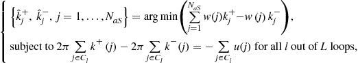 (20.49)
which is now linear with respect to the all the (positive integer) unknown ![]() and
and ![]() . It is a typical problem of Integer Linear Programming (ILP) solvable with computationally efficient techniques [60,79]. Thanks to the particular structure of the network, which is based on a triangulation, the ILP problem in (20.49) can be cast as a problem of flow optimization problem for which very efficient MCF solvers can be used. For all j, after that the integers
. It is a typical problem of Integer Linear Programming (ILP) solvable with computationally efficient techniques [60,79]. Thanks to the particular structure of the network, which is based on a triangulation, the ILP problem in (20.49) can be cast as a problem of flow optimization problem for which very efficient MCF solvers can be used. For all j, after that the integers ![]() and
and ![]() are estimated,
are estimated, ![]() is evaluated via (20.48) and used to correct the estimate of the variation over the arc of the network,
is evaluated via (20.48) and used to correct the estimate of the variation over the arc of the network, ![]() , spatial integration (which is no more dependent on the integration path) is applied to retrieve the unwrapped interferogram.
, spatial integration (which is no more dependent on the integration path) is applied to retrieve the unwrapped interferogram.
Reference [76] provides a complete comparison between the above PhU approaches.
2.20.4 Multibaseline SAR interferometry
The statistical approaches developed to solve the problem of Phase Unwrapping and SAR interferometry are based on the exploitation of the statistical model of the SAR interferometric signal [42]. The statistical techniques are in general based on the use of more than two SAR complex images (at least two interferograms) [40–42,80–82], and are often referred as multi-channel SAR Interferometry.
The basis geometry of a multi-channel SAR system is reported in Figure 20.15.
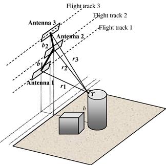
First consider the dual channel case (classical SAR Interferometry). As it has been shown in the previous sections, the actual measured values of the interferometric phase ![]() differ from the nominal ones by virtue of phase noise effects, as modeled by pdf described by Eq. (20.26). Once the data
differ from the nominal ones by virtue of phase noise effects, as modeled by pdf described by Eq. (20.26). Once the data ![]() has been observed, Eq. (20.26) can be seen as a function of the unknown parameter h, providing the single-interferogram likelihood function.
has been observed, Eq. (20.26) can be seen as a function of the unknown parameter h, providing the single-interferogram likelihood function.
The plot of the likelihood function (Eq. (20.26) as function of h) for a given measured value of the interferometric phase ![]() , and consequently of h, is shown in Figure 20.16, for two different coherence values (
, and consequently of h, is shown in Figure 20.16, for two different coherence values (![]() for the solid line,
for the solid line, ![]() for the dotted line). It shows very clearly that the likelihood function, due to its periodic nature (the period is
for the dotted line). It shows very clearly that the likelihood function, due to its periodic nature (the period is ![]() ), exhibits an infinite number of global maxima. Note also that the effect of different coherence values (the smaller the coherence value, the larger the variance of the pdf of the data) is to change the amplitude and the curvature of the likelihood function.
), exhibits an infinite number of global maxima. Note also that the effect of different coherence values (the smaller the coherence value, the larger the variance of the pdf of the data) is to change the amplitude and the curvature of the likelihood function.
Figure 20.16 Single-interferogram likelihood function for different coherence values (![]() for the solid line,
for the solid line, ![]() for the dotted line).
for the dotted line).
The Maximum Likelihood solution of the Single Interferogram InSAR problem is given by:
![]() (20.50)
(20.50)
Problem (20.50) admits the following infinite solutions [40,42,83]:
![]() (20.51)
(20.51)
as a direct consequence of the periodic nature of the likelihood function.
In order to resolve this ambiguity, we can introduce additional independent phase measures. Suppose we have multiple measures of wrapped phase ![]() , i
, i ![]() 2,…,N, obtained in N different acquisition conditions. Different wrapped phase values can be obtained, for instance, from SAR raw data acquisition from
2,…,N, obtained in N different acquisition conditions. Different wrapped phase values can be obtained, for instance, from SAR raw data acquisition from ![]() different flight track (baseline-diversity) as it is shown in Figure 20.15, or in
different flight track (baseline-diversity) as it is shown in Figure 20.15, or in ![]() sensor bands (frequency-diversity). For example, in the SIR-C/X-SAR mission X-, C-, and L-band data were acquired
sensor bands (frequency-diversity). For example, in the SIR-C/X-SAR mission X-, C-, and L-band data were acquired ![]() , while in the SRTM mission X- and C-band data were acquired (
, while in the SRTM mission X- and C-band data were acquired (![]() [50]. Each band could also be divided into sub-bands, so that
[50]. Each band could also be divided into sub-bands, so that ![]() sets of data at different frequencies could be available [42,80]. The band partition can be operated both along the range frequency band and the azimuth frequency band [42].
sets of data at different frequencies could be available [42,80]. The band partition can be operated both along the range frequency band and the azimuth frequency band [42].
Hence, the different wrapped phases are given by:
 (20.52)
where ![]() is the random process representing the phase of speckle noise at the ith antenna or in the ith band.
is the random process representing the phase of speckle noise at the ith antenna or in the ith band.
The choice of the number and kind of wrapped phase data sets, is a crucial points. A proper choice of the different flight tracks (hence, of the baselines), and/or of the different bands and sub-bands could allow to obtaining statistically independent wrapped phase data sets, as explained in Ref. [56,83]. In such case, the likelihood function relative to the single data set ![]() (n,m) is given by Eq. (20.26), evaluated at
(n,m) is given by Eq. (20.26), evaluated at ![]() and
and ![]() :
:
 (20.53)
where the dependence on (n,m) has been understood, and, in the case of N statistically independent wrapped phase data sets, the overall multi-interferogram likelihood function will be given by:
 (20.54)
where ![]() is the measured wrapped phase data vector. Note that we have a wrapped phase data vector for each position (n,m) on the ground. The plot of Eq. (20.54) for a given height value
is the measured wrapped phase data vector. Note that we have a wrapped phase data vector for each position (n,m) on the ground. The plot of Eq. (20.54) for a given height value ![]() for three values of the measured interferometric phases (suppose to consider four SAR image channels and then three interferograms), and for
for three values of the measured interferometric phases (suppose to consider four SAR image channels and then three interferograms), and for ![]() , i
, i ![]() 1,2,3, is shown in Figure 20.17. Note that the multiplication of the three single-interferogram likelihood functions, allows to avoid multiple global maxima present in each single-interferogram likelihood function, at least in the range of interest for h [83].
1,2,3, is shown in Figure 20.17. Note that the multiplication of the three single-interferogram likelihood functions, allows to avoid multiple global maxima present in each single-interferogram likelihood function, at least in the range of interest for h [83].
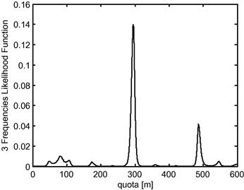
The ML estimate can be obtained by finding the unique value of h that maximize, for each position (n,m), the multi-interferogram likelihood function:
![]() (20.55)
(20.55)
The uniqueness results shown above can, in principle, also be obtained using only two interferograms: it suffices that the ratio between the period of the two single-interferogram likelihood functions is not rational, so that the overall double-frequency likelihood function is not periodic [84]. Hence, in the multi-interferogram case, the likelihood function will exhibit a single global maximum (the ML estimate).
In order to correctly implement (20.53) and (20.54), accurate knowledge of the single-interferogram likelihood functions is very important. While it can be easily obtained in the frequency-diversity case (frequencies are known with a very high precision), the same is not true for the baseline-diversity case, where baselines are known only to the precision of the inertial navigation systems, which are usually not able to achieve the required accuracy of fraction of wavelengths. A second difference is related to the fact that the different image pairs used to obtain the different wrapped phase values to be used in (20.53) are acquired in such a way that the independence of the wrapped phase values is seldom satisfied, so that model (20.54) is not valid. In this case, the determination of the multi-interferogram likelihood function would require joint statistical characterization of the different interferograms.
In Ref. [52], the joint pdf for the general case of correlated interferograms has been derived. The model given by Eqs. (20.13) and (20.14) can be generalized to the case of ![]() complex images
complex images ![]() .
.
With reference to the case of K = 3, whose geometry is shown in Figure 20.15, the interferometric phases, obtained by beating two of the three images given by Eq. (20.13) for ![]() , are:
, are:
![]() (20.56)
(20.56)
Generalizing results of Eqs. (20.16) and (20.17), the interferometric phases can be related to the observed scene height profile through:
![]() (20.57)
(20.57)
![]() (20.58)
(20.58)
Note that the three interferometric phases in Eqs. 20.56 and 20.57 are not independent each other, as each of them is univocally determined when the other two are known (f.i. ![]() . Hence, it suffices to consider only two of them. It is usually convenient considering the two interferograms obtained by referring the phase to the same master antenna, f.i. the antenna 1, then getting
. Hence, it suffices to consider only two of them. It is usually convenient considering the two interferograms obtained by referring the phase to the same master antenna, f.i. the antenna 1, then getting ![]() and
and ![]() .
.
Also in this more general multi-channel case, generalizing results relevant to two channels [52], it is possible to derive a closed form for the pdf ![]() of the interferometric speckle phase differences
of the interferometric speckle phase differences ![]() and
and ![]() [52]. Such pdf is completely symmetric respect to the interferometric phase values
[52]. Such pdf is completely symmetric respect to the interferometric phase values ![]() , and
, and ![]() , as shown in Ref. [52].
, as shown in Ref. [52].
The 2D representation of pdf ![]() is shown in Figure 20.18a, obtained with the values
is shown in Figure 20.18a, obtained with the values ![]() and
and ![]() (
(![]() , where the images coherence values have been computed according to the first order spatial decorrelation model introduced in Eq. (20.29), assuming
, where the images coherence values have been computed according to the first order spatial decorrelation model introduced in Eq. (20.29), assuming ![]() , and consequently
, and consequently ![]() , and
, and ![]() . We can notice the typical behavior met for a couple of correlated random variables. The joint pdf that would be obtained with independent interferograms, for the same parameters values used for the pdf of Figure 20.18a, is shown for comparison in Figure 20.18b.
. We can notice the typical behavior met for a couple of correlated random variables. The joint pdf that would be obtained with independent interferograms, for the same parameters values used for the pdf of Figure 20.18a, is shown for comparison in Figure 20.18b.
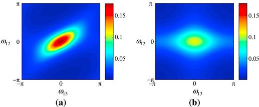
Figure 20.18 Second order pdf of dual baseline phase interferograms with ![]() , and
, and ![]() : (a) statistically dependent interferograms; (b) statistically independent interferograms.
: (a) statistically dependent interferograms; (b) statistically independent interferograms.
The 2D representation of the joint pdf ![]() for different baseline values
for different baseline values ![]() ,
, ![]() , and
, and ![]() , for
, for ![]() , and for the corresponding coherence values
, and for the corresponding coherence values ![]() ,
, ![]() , and
, and ![]() , is reported in Figure 20.19a. The joint pdf that would be obtained with independent interferograms, for the same parameters values used for the pdf of Figure 20.19a, is shown for comparison in Figure 20.19b. Note that the difference between pdfs of Figure 20.19a and b is less pronounced that the one between pdfs of Figure 20.18a and b, since in this case the statistical independence assumption is approximately met, because two of the three coherence values are very low.
, is reported in Figure 20.19a. The joint pdf that would be obtained with independent interferograms, for the same parameters values used for the pdf of Figure 20.19a, is shown for comparison in Figure 20.19b. Note that the difference between pdfs of Figure 20.19a and b is less pronounced that the one between pdfs of Figure 20.18a and b, since in this case the statistical independence assumption is approximately met, because two of the three coherence values are very low.
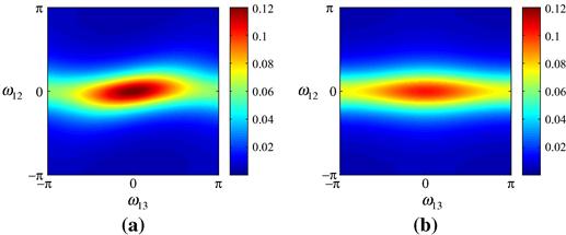
Figure 20.19 Second order pdf of dual baseline phase interferograms with ![]() , and
, and ![]() : (a) statistically dependent interferograms; (b) statistically independent interferograms.
: (a) statistically dependent interferograms; (b) statistically independent interferograms.
Also in this case the interferometric phases pdf can be obtained through a change of variables, generalizing what described for one variable in Eq. (20.26):
![]() (20.59)
(20.59)
The differences evidenced in Figures 20.18 and 20.19 for the speckle phases, with and without correlation, result also in the case of the interferometric phases ![]() and
and ![]() . In some conditions, the differences between the two cases pdfs can be more pronounced, in other less. Of course, in case of significantly correlated interferograms, the height estimation according (20.55) by using the joint pdf of independent interferograms (Eq. (20.54) in place of (20.59)) would lead to larger estimation errors both in terms of quadratic errors and bias, especially when the two joint pdfs assumes very different shapes [85]. Equation (20.59), which can be easily generalized to the case of more than two interferograms [52], is very general, and reduce to (20.54) in the case of independent (and hence, uncorrelated) interferograms.
. In some conditions, the differences between the two cases pdfs can be more pronounced, in other less. Of course, in case of significantly correlated interferograms, the height estimation according (20.55) by using the joint pdf of independent interferograms (Eq. (20.54) in place of (20.59)) would lead to larger estimation errors both in terms of quadratic errors and bias, especially when the two joint pdfs assumes very different shapes [85]. Equation (20.59), which can be easily generalized to the case of more than two interferograms [52], is very general, and reduce to (20.54) in the case of independent (and hence, uncorrelated) interferograms.
Use of pdf (20.59) in place of (20.54) allows to obtain better results in terms of accuracy (Bias and Cramer-Rao Lower Bounds) of the reconstructed ground height profiles [52,85].
2.20.4.1 Bayesian statistical solution to PhU problem
To solve the problem of the estimation of the ground elevation profile also Bayesian statistical techniques have been proposed [86–88]. In the framework of such techniques, in particular if a Maximum a Posteriori (MAP) estimation scheme is adopted, an a-priori joint pdf of the unknown height profile has to be introduced. It is based on the use of Markov Random Fields (MRF) as a-priori statistical term modeling pixels contextual statistical information in the 2D unknown height profile to be reconstructed. The MRF allows to describe the local spatial interaction between couples of pixels, through a set of model parameters (hyperparameters) which can be tuned following unsupervised procedures.
Consider a discrete (lexicographically ordered) two-dimensional (2D) points lattice ![]() , where
, where ![]() is the number of pixels of the SAR image, and let
is the number of pixels of the SAR image, and let ![]() the corresponding ground elevation values. Consider now an InSAR system, and let
the corresponding ground elevation values. Consider now an InSAR system, and let ![]() the wrapped phase values (single sample of a discrete interferogram) measured at the lattice point k and at nth interferogram. The wrapped phase values
the wrapped phase values (single sample of a discrete interferogram) measured at the lattice point k and at nth interferogram. The wrapped phase values ![]() relative to the position k can be structured and ordered in the following way: let
relative to the position k can be structured and ordered in the following way: let ![]() be the vector of the wrapped phases measured in k position at the N different interferograms, and
be the vector of the wrapped phases measured in k position at the N different interferograms, and ![]() be the vector collecting all available wrapped phase values. Then, h is the vector of the unknown height values, and
be the vector collecting all available wrapped phase values. Then, h is the vector of the unknown height values, and ![]() the vector of the all available data (multi-interferogram).
the vector of the all available data (multi-interferogram).
The MAP estimation can be formulated as:
![]() (20.60)
(20.60)
where ![]() is the a posteriori joint pdf of the unknown image,
is the a posteriori joint pdf of the unknown image, ![]() is the Bayesian likelihood function [89], and
is the Bayesian likelihood function [89], and ![]() is the a-priori pdf of the unknown image.
is the a-priori pdf of the unknown image.
The Bayesian likelihood function can be easily obtained by Eq. (20.59):
 (20.61)
where the statistical independence of the interferograms in the different ground positions ![]() has been exploited. The Bayesian likelihood functions are formally equal to the likelihood function that can be obtained in the classical statistical case; in the Bayesian framework, differently from the classical one, the unknown image is seen as a sample of a random vector H.
has been exploited. The Bayesian likelihood functions are formally equal to the likelihood function that can be obtained in the classical statistical case; in the Bayesian framework, differently from the classical one, the unknown image is seen as a sample of a random vector H.
The a-priori pdf ![]() is usually defined in such a way to express a-priori information about the unknown image, assigning high probability to particular pixels configurations. In the SAR interferometry case, being the unknown image representative of the ground elevation map of a geographic area, a strong contextual pixel information is very likely to be. In particular, it can be assumed that the unknown image can be modeled as a Markov Random Field (MRF) [90], a general image model able to represent contextual pixel information extending the 1-D Markov property to the 2-D case, whose corresponding joint pdf is given by a Gibbs distribution:
is usually defined in such a way to express a-priori information about the unknown image, assigning high probability to particular pixels configurations. In the SAR interferometry case, being the unknown image representative of the ground elevation map of a geographic area, a strong contextual pixel information is very likely to be. In particular, it can be assumed that the unknown image can be modeled as a Markov Random Field (MRF) [90], a general image model able to represent contextual pixel information extending the 1-D Markov property to the 2-D case, whose corresponding joint pdf is given by a Gibbs distribution:
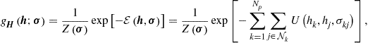 (20.62)
where ![]() is the so-called partition function (a constant factor needed to normalize the integral of the pdf to one),
is the so-called partition function (a constant factor needed to normalize the integral of the pdf to one), ![]() is the energy function,
is the energy function, ![]() is the potential function between
is the potential function between ![]() and
and ![]() is the neighbourhood system of kth pixel [91] (usually, the eight pixels around the kth one),
is the neighbourhood system of kth pixel [91] (usually, the eight pixels around the kth one), ![]() is the hyperparameter vector, and
is the hyperparameter vector, and ![]() are the hyperparameters. With such definition, the Gibbs-MRF model in Eq. (20.62), by means of the hyperparameters, well adapts to describe the image local nature, leading to a powerful and general model, well-suited to represent a very wide class of height profiles. The hyperparameter values are not know, of course, and they have to be estimated from the available interferometric data
are the hyperparameters. With such definition, the Gibbs-MRF model in Eq. (20.62), by means of the hyperparameters, well adapts to describe the image local nature, leading to a powerful and general model, well-suited to represent a very wide class of height profiles. The hyperparameter values are not know, of course, and they have to be estimated from the available interferometric data ![]() data.
data.
The solution procedure essentially consists of two steps: ML estimation (![]() of the hyperparameter vector
of the hyperparameter vector ![]() and MAP estimation (
and MAP estimation (![]() of the actual realization of height profile process H.
of the actual realization of height profile process H.
This approach can work very well [87], even if the method is always limited by the coherence value and by the corresponding number of available independent acquisitions of the same scene. The lower are the coherence values over the entire image, the larger is the total number N of needed interferograms to obtain good quality reconstructions.
Performance of the Bayesian method can significantly outperform the one relevant to classic approaches [85,92] depending on the capability to estimate the a-priori model of the unknowns.
2.20.4.2 Graph cuts solution to PhU problem
Statistical approaches, especially the Bayesian ones, have proved to be effective dealing with noisy data and big discontinuities. However these algorithms can be time consuming and computationally heavy due to the a-priori model (estimation of hyperparamenters) and to the optimization step. It is possible to overcome these limits by introducing a fast and efficient (in term of global optimization) algorithm to unwrap the interferometric phase in the multichannel configuration [85].
To reduce the computational time needed to unwrap the multichannel interferometric phase, two aspects can be taken in consideration: first, a non-local a-priori energy function, the Total Variation (TV) model [93], and secondly an optimization algorithm based on graph cuts, Ishikawa algorithm [94], have been exploited.
The a-priori energy corresponding to the TV model can be written as follows:
 (20.63)
Note that in this expression, ![]() is a scalar, making model in Eq. (20.63) a non local one, differently from the Bayesian model (20.62) presented in the previous section. This choice is done in order to make the algorithm faster. A non local a-priori model avoids the estimation of local hyperparameters
is a scalar, making model in Eq. (20.63) a non local one, differently from the Bayesian model (20.62) presented in the previous section. This choice is done in order to make the algorithm faster. A non local a-priori model avoids the estimation of local hyperparameters ![]() , as only one parameter
, as only one parameter ![]() for the whole image has to be estimated.
for the whole image has to be estimated.
Between the existing non local a-priori energy models, TV has been chosen, due to its main advantage: TV does not penalize discontinuities in the image while simultaneously not penalizing smooth functions either [93].
Given the TV a-priori energy model (20.63), the MAP estimation can be obtained from the minimization of the following function:
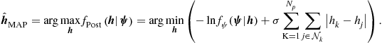 (20.64)
In order to minimize this energy function, graph-cut based optimization algorithms are used. Graph-cut optimization [95,96] is successful because the exact minimum or an approximate minimum with certain guaranties of quality can be found. Compared to the classical optimization algorithm, it provides comparable results with much less computational time and compared to the deterministic algorithm ICM [90], it avoids the risk of being trapped in local minima solution which can be far from the global one.
Let us, first, define a graph and a graph-cut problem. Suppose ![]() is a directed graph with non negative edge weights, where V is the set of vertexes and E the set of edges. This graph has two special vertexes (terminals) called the source s and the sink t. A s-t-cut C = {S,T} is defined as a partition of the vertexes into two disjoint sets S and T such that s
is a directed graph with non negative edge weights, where V is the set of vertexes and E the set of edges. This graph has two special vertexes (terminals) called the source s and the sink t. A s-t-cut C = {S,T} is defined as a partition of the vertexes into two disjoint sets S and T such that s ![]() S and t
S and t ![]() T. A cost of this cut is defined as the sum of weights of all edges that go from S to T. Figure 20.20a shows a simple graph made of four vertexes, two vertexes (x,y) plus the sink and the source (t,s). The edges are the links between the vertexes. An example of a cut is represented with the dashed line.
T. A cost of this cut is defined as the sum of weights of all edges that go from S to T. Figure 20.20a shows a simple graph made of four vertexes, two vertexes (x,y) plus the sink and the source (t,s). The edges are the links between the vertexes. An example of a cut is represented with the dashed line.

Figure 20.20 (a) Example of a graph construction and of a cut on it (dashed line); (b) Ishikawa Graph Construction—On the axes there are the pixels and the labels; data edges are depicted as black arrows; constraint edges are represented by horizontal arrows and penalty edges are depicted as dotted arrows; (c) Ishikawa edges weights—Representation of the edges for a vertex.
The minimum s-t-cut problem is to find a cut C with the smallest cost. This problem is exactly equivalent to its dual problem, which consists in computing the maximum flow from the source to the sink. Between the several algorithms proposed to solve the maximum flow problem, the one proposed in [97] turns to be the most adapted to computer vision problems.
To solve the MAP unwrapping problem, which means find the value of h that minimizes (20.64) the optimization procedure proposed by Ishikawa is implemented [94]. The interesting aspect of Ishikawa algorithm is that under some hypothesis on the energy to be minimized and if the graph is correctly constructed, the algorithm provides the global optimum of the considered energy.
Two hypothesis are at the base of Ishikawa algorithm: convexity of the a-priori energy and a linear order on the label set. Using the TV model the first hypothesis is satisfied. For the second hypothesis, in the case of phase unwrapping, the labels are the height of the image pixels. The heights are supposed to be represented as integers in the range {0,1,2,..,L−1}, where L is the size of the label sets. This condition satisfies the second hypothesis necessary for the Ishikawa graph construction.
Ishikawa method is based on computing a minimum cut in a particular graph. Ishikawa graph G = (V,E) contains ![]() nodes (
nodes (![]() is the size of the image and L is the size of the label set) denoted by {
is the size of the image and L is the size of the label set) denoted by {![]() }, plus two special nodes s and t. For each pixel k, we associate L nodes, that represent all the possible heights that the pixel k can take. The construction of Ishikawa graph, in case of a 1D image for legibility, is shown in Figure 20.20b.
}, plus two special nodes s and t. For each pixel k, we associate L nodes, that represent all the possible heights that the pixel k can take. The construction of Ishikawa graph, in case of a 1D image for legibility, is shown in Figure 20.20b.
Ishikawa graph contains three families of edges ![]() .
. ![]() is a set of directed edges called data edges (black arrows of Figure 20.20b). It represents the data energy term.
is a set of directed edges called data edges (black arrows of Figure 20.20b). It represents the data energy term. ![]() is a set of directed edges called penalty edges (dotted arrows of Figure 20.20b). It ensures that only one data edge is in the minimum cut for each pixel k. Finally,
is a set of directed edges called penalty edges (dotted arrows of Figure 20.20b). It ensures that only one data edge is in the minimum cut for each pixel k. Finally, ![]() is a set of constraint edges between all neighbor pixels (horizontal arrows in Figure 20.20b). It represents the a-priori energy term.
is a set of constraint edges between all neighbor pixels (horizontal arrows in Figure 20.20b). It represents the a-priori energy term.
To better understand how to set the edges weight for the multichannel phase unwrapping problem let us consider Figure 20.20c. The vertex ![]() is the vertex identified by the pixel k and the label l. The cost of the edges in Ishikawa graph are reported in Eq. (20.65). For more details on the graph construction see [94].
is the vertex identified by the pixel k and the label l. The cost of the edges in Ishikawa graph are reported in Eq. (20.65). For more details on the graph construction see [94].
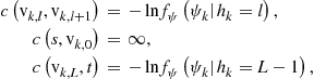 (20.65)
![]()
Constructing the Ishikawa graph as shown and finding the cut with a minimum cost on this particular graph allows to find the exact (global) optimum solution for the multichannel phase unwrapping problem given by Eq. (20.64). The main disadvantage of Ishikawa method is related to the memory load. In fact, the algorithm stores the whole graph and then performs the cut. This can be a problem when the size of the images largely increase.
Before using Ishikawa algorithm, the hyperparameter ![]() has to estimated. The hyperparameter
has to estimated. The hyperparameter ![]() depends both on data energy and on a-priori energy term. A method to perform the hyperparameter parameter is the analysis of the so called L-curve. To find automatically the corner of the L-curve, the triangular method described in [98] can be used, providing good results in limited time.
depends both on data energy and on a-priori energy term. A method to perform the hyperparameter parameter is the analysis of the so called L-curve. To find automatically the corner of the L-curve, the triangular method described in [98] can be used, providing good results in limited time.
2.20.5 Multipass interferometry
Advanced differential SAR interferometric (A-DInSAR) techniques process multitemporal data, acquired over repeat passes, to generate very accurate deformation time series and therefore to achieve a regular monitoring of the deformation of the observed scene. A-DInSAR techniques also mitigate most of the limitations of the standard single-interferogram approaches, such as temporal and geometric decorrelation and the atmospheric phase delay and, unlike conventional Interferometry, they allow increasing the measurement accuracy from centimeter up to millimeter. These techniques also improve standard approaches both in terms of deformation modeling capabilities and quality measurements.
We refer to the geometry depicted in Figure 20.21, where we assume that the satellite is collecting the data at time instants ![]() , with baselines
, with baselines ![]() , with respect to a reference image.
, with respect to a reference image.
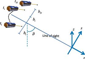
Let ![]() be the vector that collect the phase measurements,
be the vector that collect the phase measurements, ![]() . The following data model is assumed:
. The following data model is assumed:
![]() (20.66)
(20.66)
where ![]() is a vector of a-dimensional parameters that collect the angular variations corresponding to the baseline distribution
is a vector of a-dimensional parameters that collect the angular variations corresponding to the baseline distribution ![]() , d is the vector collecting the displacements at the different times,
, d is the vector collecting the displacements at the different times, ![]() ,
, ![]() , and
, and ![]() are respectively the unwanted vectors collecting the APD, also known as Atmospheric Phase Screen (APS) [74], the orbit errors and the noise, which, in this case, includes also the temporal decorrelation effects in addition to the spatial decorrelation contribution due to the speckle. Note that the elevations can be related to the target height z as s = h/sin (
are respectively the unwanted vectors collecting the APD, also known as Atmospheric Phase Screen (APS) [74], the orbit errors and the noise, which, in this case, includes also the temporal decorrelation effects in addition to the spatial decorrelation contribution due to the speckle. Note that the elevations can be related to the target height z as s = h/sin (![]() ).
).
The final aim of multipass DinSAR techniques is to reconstruct d, and especially for some specific applications to estimate s to correctly localize the target to which the displacements refer. In doing this the cancellation of the unwanted disturbance terms is carried out by using a proper modeling, of deterministic nature (such as for instance the baseline dependent term related to the target elevation and the orbit error which show a predictable spatial variability) and stochastic models, such as for the characterization and filtering of the atmospheric component.
Some remarks are now in order. First of all the phase of each single SAR image depends on the phase of the backscattering coefficient that, for distributed scatterers, can be strongly variable from pixel to pixel. Therefore interferograms must be formed in such a way to mitigate, as much as possible the effects of the backscattering coefficient. Secondly, the interferograms are extracted by complex numbers and therefore the phase values are wrapped, i.e., they are determined only on a basic interval of 2![]() size.
size.
With regards to the process of determining the set of interferogram to be used for the displacement estimation process, there are essentially two alternative options: the (temporal) Persistent Scatterers Interferometry (PSI) and the (spatial) Coherent Scatterers Interferometry (CSI) approaches. Almost all implementations of these class of approaches makes use of the model in Eq. (20.66).
The main difference between the two approaches is the basic assumption underlying the typology of the scattering which impacts the strategy followed in the interferogram generation and in the scale of analysis.
In the PSI case the interferometric analysis is carried out at the highest possible spatial resolution, the set of interferograms is generated with respect to the master image without taking any care to avoid large spatial and temporal baselines. This strategy is chosen in PSI because the technique is aimed at monitoring the deformation of dominant scatterers, i.e., of scatterers showing a persistency of the scattering mechanism over the time. Many natural reflectors, typically present over man-made structures, satisfy this requirement. In the PSI approach the use of large spatial baselines are functional to the achievement of a high accuracy in the estimation of the target elevation which provides a high accuracy in the localization of ground scatterers and therefore in the identification of the scatterers subject to possible deformations.
Most of PSI algorithms rely on the use of simplified version of the model in (20.66) in which the deformation is assumed to be linear i.e., ![]() where v is the deformation mean velocity and t is the vector collecting the time instants.
where v is the deformation mean velocity and t is the vector collecting the time instants.
In this case the phase vector ![]() is expressed as:
is expressed as:
![]() (20.67)
(20.67)
From Eqs. (20.66) and (20.67) it is evident that, besides the linear deformation approximation, other two assumptions are fundamental: that is the possibility to neglect the atmospheric contribution and the orbital inaccuracy. While the latter assumption does not play a critical role because the orbital errors are rather accurately modeled as spatial (azimuth-range) planar phase contributions that can be accurately estimated and compensated directly on the measured complex data in wide areas, neglecting the atmospheric phase pattern is a main issue. One possibility to handle the atmospheric contribution is by exploiting its the spatial correlation properties, specifically the fact that contributions on a scale of a few hundreds of meters are strongly correlated as explained in Section 2.20.3.3. Accordingly, this contribution can be estimated on a coarse grid and subtracted from the data. In the case of the original Persistent Scatterers algorithm of [99,100], the grid of pixels used for the estimation of the atmospheric phase pattern is selected by measuring the amplitude dispersion index, which is a proxy of the phase stability.
Following this compensation each pixel is investigated for the presence of scatterers with “persistent” properties, i.e., a parameter that describes the fit between the model and the real phase is considered:
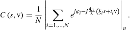 (20.68)
Equation (20.68) provides a normalized (in the [0,1] interval) measure, of the temporal (i.e., persistent) coherence property of scatterers: s (scatterer elevation) and v (velocity) are unknowns that are determined via a maximization
![]() (20.69)
(20.69)
It is interesting to note that by letting:
![]() (20.70)
(20.70)
where ![]() is the jth component of
is the jth component of ![]() .
.
Now, introducing:
![]() (20.71)
(20.71)
where ![]() is the jth component of
is the jth component of ![]() , and
, and ![]() is the jth component of t.
is the jth component of t.
Then Eq. (20.68) can be rewritten as:
![]() (20.72)
(20.72)
This equation highlights the fact that the PS approach uses indeed with unitary weighting all the interferograms ![]() , and therefore the whole information available in the data is used in the determination of the target height and velocity.
, and therefore the whole information available in the data is used in the determination of the target height and velocity.
Since the proposal of the PS technology, many other PSI techniques have been proposed: SPN [101], PSI-GENESIS [102], IPTA [103], SPINUA [104]. In most of the cases they differ essentially in the selection of the sparse grid over which the interferometric analysis is carried put. A solution that extensively use the model in (20.67) is the Persistent Scatterers Pairs (PSP) algorithm [105]. In this case the mitigation of the atmospheric contribution is carried out by considering the phase variation over spatial arcs: the atmospheric contribution as well as non-linear effects spatially slowly variable are automatically canceled provided that the length of the arc is sufficiently small. In the PSP case, the selection of the sparse grid of analysis is carried out by moving from a reference starting point to the adjacent points using the spatial arcs and the model in (20.67).
The capability of SAR to monitor deformation phenomenon up to centimeters by compensating topography and atmospheric disturbances via processing of stacks of data was for the first time provided by the group of Politecnico of Milan with the persistent scattereres technique. The examples included in the seminal papers [99,100] that demonstrated for the very first time the possibility to monitor demonstration with millimeter per year accuracy of to the Pomona (CA-USA). Among the first examples of application of the Persistent Scatterers is the monitoring of the Etna volcano (see Figure 20.22).
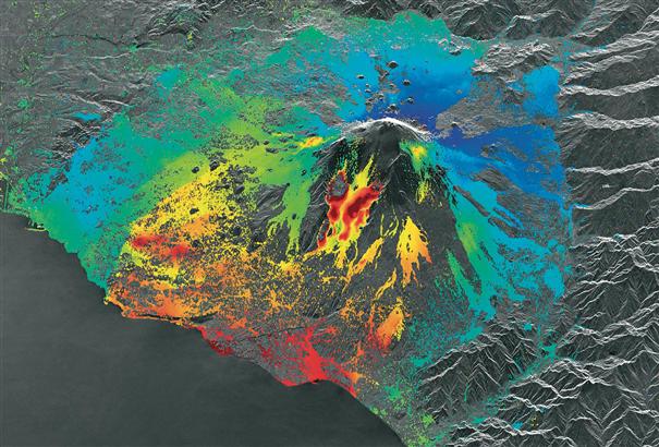
Figure 20.22 The persistent scattereres technique applied to the monitoring of the Etna volcano in the period 1995–1999, colorbar is saturated in the range (−30,30) mm/yr.Tele-Rilevamento Europa (T.R.E. s.r.l.) and Politecnico of Milano.
Currently Multipass DInSAR techniques, such as small baseline and persistent scatterers are applied to monitor deformation phenomena associated in seismogenetic areas [106], landslides [107], areas affected by underground excavation or water level changes [108] gas pumping and storage, etc. over wide areas.
An example of application of PSI on a national scale is provided in Figure 20.23.

Figure 20.23 Result of the PST project funded by the Italian Ministery of the Environment for monitoring the displacements in Italy via the Persistent Scatterers Interferometry technique. Data of the ESA ERS-1 and ERS-2 satellites.TREuropa.
Multipass DinSAR techniques allows also image and monitor ground scatterers with high spatial resolution. Persistent Scatterers Interferometry (PSI) techniques exploits all the available acquisitions in such a way to improve the performances with respect to this specific case.
PSI approach are designed to monitor deformation of dominant scatterers. PSI may however loose the capability of monitoring scatterers which shows non negligible temporal or spatial decorrelation: such scatterers are corresponding to areas in which the scattering is not concentrated in a dominant point but rather is distributed over the resolution cell.
Techniques complementary to PSI that uses only interferograms showing a sufficient high degree of spatial coherence [109–111], in this work referred to as coherent stacking interferometric (CSI) techniques, aims to overcome the problems of PSI related to distributed scattering.
In fact, following the lines of the classical (single-pair) DInSAR analysis, CSI techniques carry out an analysis of multilook interferograms: the multilook operation, i.e., a spatial averaging which is carried out by exploiting the hypothesis that the scattering is distributed, allows on one side accessing a measure of quality of the signal in each interferogram, i.e., the spatial coherence, and on the other side it allows increasing the signal phase quality though the averaging operation.
The first interferometric stacking technique proposed in the literature has been the Small BAseline Subset (SBAS) technique [109]. This technique makes use of a limitation on the spatial and temporal baselines to control the temporal and geometric (also known as angular) decorrelation phenomena which is more critical in the presence of distributed scattering.
As described in Section 2.20.3.2 geometrical decorrelation is a phenomenon which is associated with the fact that even small variations of the radar line of sight direction in the elevation direction induced by the orbital separation (spatial baseline decorrelation) and/or aspect angle (induced by doppler centroid vatiation); temporal decorrelation is due to changes over the time of the scattering. The SBAS technique uses only interferograms generated by choosing thresholds on the spatial and temporal baselines, that is the spatial orbital and temporal separations, respectively, and on the Doppler centroid difference (for systems suffering of large variation of the Doppler centroid) thus limiting the effects of angular and temporal decorrelation. Mathematically, letting ![]() the vector that collects the M (multilook) interferograms values in a generic pixel, we have:
the vector that collects the M (multilook) interferograms values in a generic pixel, we have:
![]() (20.73)
(20.73)
where ![]() is the multilook version of
is the multilook version of ![]() and A is a
and A is a ![]() matrix
matrix ![]() incidence matrix that describes the structure of the interferogram stack used in the processing: it is dependent on the pairing of the acquisitions in the interferogram generation. Equation (20.73) refers to the absolute phase values: hence the set of interferogram is unwrapped, (commonly via the Minimum Cost Flow algorithm [58–60,79]) and then (20.73) is inverted pixel by pixel to retrieve the phase signal over the stack of acquisitions.
incidence matrix that describes the structure of the interferogram stack used in the processing: it is dependent on the pairing of the acquisitions in the interferogram generation. Equation (20.73) refers to the absolute phase values: hence the set of interferogram is unwrapped, (commonly via the Minimum Cost Flow algorithm [58–60,79]) and then (20.73) is inverted pixel by pixel to retrieve the phase signal over the stack of acquisitions.
The SBAS approach, by using the Singular Value Decomposition [112] technique allows also handling the case in which, due to the limitations on the baselines, the acquisitions are grouped in different independent subsets leading to the case of ill-conditioning of the matrix A in (20.73). This latter feature allows also performing a “semi-coherent” combination of data of different sensors (f.i. ERS and ENVISAT), i.e., the combination of sets of coherent data for which are incoherent each other.
It is worth pointing out that the system in (20.73) is intrinsically invertible for each pixel up to a constant: typically this constant is set in such a way to have a null deformation at time ![]() . Moreover, as each interferogram is known up to a constant phase value, the solution of (20.73) for all pixels is known up to the deformation of a known point which must be set, as in classical leveling technology, as a reference point. After the inversion the deformation time series are separated from atmospheric contribution by using (20.66): in particular the deformation mean velocity and the residual topography are estimated by assuming for
. Moreover, as each interferogram is known up to a constant phase value, the solution of (20.73) for all pixels is known up to the deformation of a known point which must be set, as in classical leveling technology, as a reference point. After the inversion the deformation time series are separated from atmospheric contribution by using (20.66): in particular the deformation mean velocity and the residual topography are estimated by assuming for ![]() the model in (20.67). The linear motion and topography errors are subtracted from the data and the residuals are then filtered to separate the non-linear deformation component from the APD contribution: this separation relies on the assumption that the deformations are typically correlated spatially and temporally (slow deformations) whereas the atmosphere is spatially correlated but almost independent from epoch to epoch. The latter assumption is certainly valid for the turbulent component of the APD whereas it may be critical in case of dense temporal sampling (i.e., low revisiting time) for the stratified contribution (depending on the topography) which exhibit seasonal dependencies.
the model in (20.67). The linear motion and topography errors are subtracted from the data and the residuals are then filtered to separate the non-linear deformation component from the APD contribution: this separation relies on the assumption that the deformations are typically correlated spatially and temporally (slow deformations) whereas the atmosphere is spatially correlated but almost independent from epoch to epoch. The latter assumption is certainly valid for the turbulent component of the APD whereas it may be critical in case of dense temporal sampling (i.e., low revisiting time) for the stratified contribution (depending on the topography) which exhibit seasonal dependencies.
Differently from the SBAS approach where typically a degree of redundancy is imposed at the interferogram generation level to control the presence of possible unwrapping errors, the CPT technique uses a Minimum Spanning Three [113] strategy to connect the acquisition stack, and therefore to generate the interferograms. Another special feature of the CPT approach is related to the implementation of a step which allows, via modeling, to retrieve the linear deformation component and DEM error contribution prior to extraction of the non-linear component. In this sense the technique is very similar to the ESD approach proposed in [114].
The A-DinSAR techniques working at lower resolution, such as SBAS and CPT, allows to easily implement a two-stage, low-resolution and high-resolution, interferometric processing strategy for the evaluation of the deformation over at small and a high scale, respectively.
In other words, once the atmospheric phase component and the non-linear deformation are extracted, they are subtracted from the original data corresponding to each acquisition at full resolution. Such data can be used in conjunction with the model in (20.67) to perform, as in standard PSI, the estimation of the deformation at full resolution. It is worth noting that, due to the fact that the increase of resolution is aimed at analyzing dominant scatterers, it is not convenient at this stage the introductions of limitation on the baselines. Moreover, whereas common band filtering may be beneficial to counteract the geometrical decorrelation effect in case of distributed scattering, for the full resolution analysis tuned to dominant scattering such filtering can be deleterious because in this case it cannot be assumed that spectral components of the scattering mechanism are still independent.
A possibility that provides improved performances in the full resolution analysis is given by the use of imaging techniques. Based on a tomographic processing, multidimensional SAR imaging use both the amplitude and phase values of the received signal to perform a full resolution analysis that allows increasing the detection performances of persistent scatterers, as well as the estimation of their associated parameters, i.e., the velocity and the elevation. Furthermore, by analyzing the scattering distribution in the elevation/velocity plane, they allows identifying and separating the contributions of scatterers which are interfering in the same pixel. The interference of scatterers is particularly critical in the case of complex scenarios such as urban areas, in which the phenomenon of layover affect all the vertical structures. These topics are the subject of the SAR Tomography and Differential SAR Tomography techniques which are discussed in details later on.
Figure 20.24 provides an example of application of the SBAS based approach to the monitoring of wide areas [115]. Many deformation phenomena corresponding to natural hazard are evident (the Campi Flegrei caldera subsidence in Naples, the Colli Albani uplift in the south of Rome, etc.). Besides providing the measurement of deformation associated with progressive and regular hazard sources, such as subsidence due to water pumping, regular volcanic activities, etc., the multipass SAR technique is also particularly important in the post crisis phase. The recent literature includes many examples of application of the multipass DInSAR technique to the monitoring of post-seismic deformation. One of the most effective example of monitoring of post-seismic deformation is provided by the CSK constellation with reference to the l’Aquila earthquake. Starting from April 6th, 2009 date the CSK constellation (at that time operative with three satellites) was capable in six months to acquire different dataset with a rate that, for the best dataset, was the highest possible, i.e., about 1 acquisition each 5 days on average.

Figure 20.24 Example of a wide area monitoring using by combining the results of 3 ERS-Envisat frames from Naples to Rome.
Figure 20.25 shows the image corresponding to the mean post-seismic velocity: the red spot shows the deformation in correspondence of the Paganica San Demetrio fault. The time series also shows very clearly the typical exponentially decreasing post-seismic deformations.
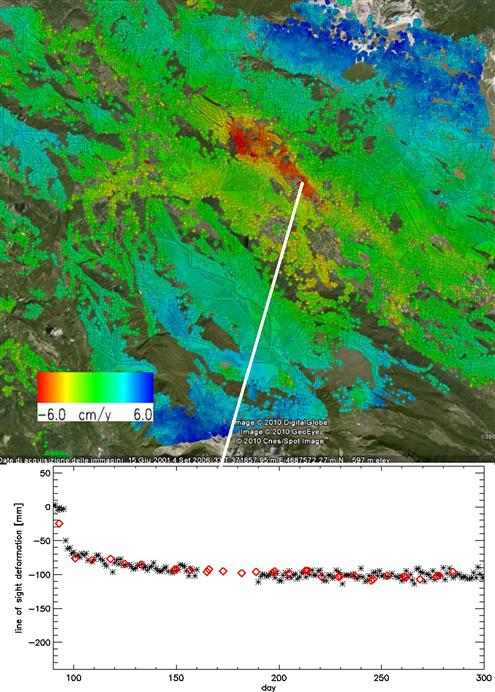
Figure 20.25 Post-seismic deformation monitoring over the l’Aquila area. Upper image: post-seismic mean deformation velocity. Lower image: comparison between GPS (black stars) and SAR measurements (red diamonds) [116]. (For interpretation of the references to color in this figure legend, the reader is referred to the web version of this book.)
Particularly relevant are the effects of uplift which are observed on the mountainous areas in the North and South area. Such effects are an evidence of the effects of the non-turbulent (stratified) component of the troposphere corresponding to the hydrostatic path delay, and show a seasonally variability. It is worth to note that the reduction of the wavelength with respect to C-Band data X-Band systems such as COSMO/SKYMED and TerraSAR-X, on one side provides a higher sensitivity to deformation, on the other side it introduces an amplification of the range variation component associated with ADP. The tropospheric component under investigation cannot be filtered via a simple approach based on the temporal independence of APD, as done in the classical multitemporal interferometric processing scheme described above. Such effects, whose compensation is of main importance for the application in emergencies situations (in which typically a few acquisitions are available), can be handled either by using external tropospheric delay measurements, provided for instance by GPS networks, of by subtracting from the interferograms the components highly correlated to the topography: the latter solution may be critical in cases in which the deformation signal is itself correlated with the topography (for instance, volcanoes inflation).
A final example of application of multitemporal DInSAR analysis is provided by the use of PSI on data acquired by the last generation, high resolution satellites. In Figure 20.26 it is shown the result of PSI applied to four ascending and descending tracks acquired by the TerraSAR-X system operating in the spotlight mode over the Berlin station. The figure provides the measurement of deformation caused by thermal dilations. At certain positions along the rail track, there is a ![]() phase change. At these locations rail expansion joints are installed and the rail tracks dilate horizontally and in opposite directions.
phase change. At these locations rail expansion joints are installed and the rail tracks dilate horizontally and in opposite directions.
Figure 20.26 Geocoded persistent scatterers obtained from a fusion of 4 different stacks (ascending & descending) of TerraSAR-X high resolution spotlight data [117]. Colors represent estimated amplitudes of seasonal deformation in west-eastern direction in the interval [+7, −7] mm.DLR and Technical University of Munich (TUM), Germany.
2.20.5.1 Multipass phase unwrapping
As already stated in Section 2.20.4, Phase Unwrapping is necessary to extract the APD component and to estimate the non-linear deformation signal at either small or large scale: PhU is by far the most critical step of any A-DInSAR technique.
Most of PhU algorithms have been developed in the context of SAR Interferometry, and make use of the pixel-to-pixels spatial variations. One of the most used algorithm is the Minimum Cost Flow (MCF) PhU [60,79]: it is based on the use of triangulations defined on the sparse grid of useful pixels and the PhU is cast as the problem to minimize the L1 norm of a vector that corrects the measured phase differences subject to the zero-curl (i.e., non rotational) constraint, that is the constraint that forces to zero the circulation of the unwrapped phase differences on all the triangles. Very efficient MCF solvers are available in the framework of network-flow algorithms [60].
The MCF technique, typically exploited for the unwrapping of single interferograms, has been also extensively used in the multitemporal DInSAR context where commonly several interferograms must be unwrapped. More specifically, phase unwrapping of DInSAR data stacks is carried out by independently unwrapping each interferogram with the MCF optimization approach (single-step PhU).
The single-step PhU discards any relationship between the different interferograms, which are indeed all related to the same wanted signals; particularly it neglects the typical inherent redundant nature of the interferogram stack.
To overcome this limitation, the single-step PhU has been recently integrated with Model Based (MB) phase unwrapping algorithm that exploits the model in (20.67) also at the phase unwrapping stage. More specifically, starting from the measured interferograms, the MB PhU estimates the variations of the topography (![]() and deformation mean velocity (
and deformation mean velocity (![]() over the set of spatial arcs defined on a grid of reliable pixels, i.e., with a coherence degree [118] which is above a threshold for a fixed percentage of the total number of interferograms:
over the set of spatial arcs defined on a grid of reliable pixels, i.e., with a coherence degree [118] which is above a threshold for a fixed percentage of the total number of interferograms:
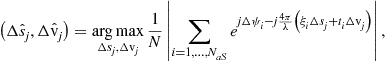 (20.74)
where ![]() is the variation of the wrapped phase measured on the jth (out of
is the variation of the wrapped phase measured on the jth (out of ![]() spatial arc.
spatial arc.
The set of all measured topography and deformation mean velocity deformation mean velocity, ![]() and
and ![]() , are then spatially integrated (generally in a Least-Square sense) over the network associated with the spatial arcs to retrieve the topography and deformation mean velocity at the pixel level. The phase signal corresponding to the signal component model is subtracted from each interferogram to ease the subsequent un-modeled unwrapping step, generally carried out with the application of the MCF algorithm applied independently to the each of the available interferograms [115,119].
, are then spatially integrated (generally in a Least-Square sense) over the network associated with the spatial arcs to retrieve the topography and deformation mean velocity at the pixel level. The phase signal corresponding to the signal component model is subtracted from each interferogram to ease the subsequent un-modeled unwrapping step, generally carried out with the application of the MCF algorithm applied independently to the each of the available interferograms [115,119].
Recently new algorithms has been proposed to improve the un-modeled PhU stage by exploiting the redundant nature of the interferograms [120–122].
A first contribution along this line is the two step PhU algorithm [122], where the use of a triangulation is in the spatial temporal baseline domain, see Figure 20.27, is used: each point represents an acquisition and arcs represents the interferograms. For each spatial arc, the interferometric measurements available in all the interferograms provide an estimate of the phase variations over the acquisition arcs in Figure 20.27. It is clear therefore that such phase variations must sum up to zero over closed circuits and therefore an MCF step can be therefore carried out in the acquisition domain to provide corrections of the phase variation over the selected spatial arc in each interferograms which are used for the subsequent MCF PhU implemented, as usual, in the spatial domain.

This two-step approach has the advantage to use the redundancy of the available interferograms, phase summation of interferograms over close loop should be zero, but imply a rigid scheme in the interferogram generation. The use of a triangulation does not allow fixing a limit to the baseline separation, as usually done in the SBAS approach, because the maximum baseline is defined by the triangulation scheme.
A solution to tackle problem is obtained by address the PhU problem in a generalized framework which makes use of the over-determined nature of the operator that relates the phase differences to the absolute phase values, [119]. More specifically, by referring to Figure 20.28 where a 3D representation of the stack of acquisition is shown, we let l and n indicating the pixel and the acquisition, respectively, and j the spatial arc. It is possible to define two operators implementing a differentiation along the acquisition (i.e., the interferogram generation) and along the space (spatial variation). A generic estimation of the absolute phase variation over the mth interferogram obtained by wrapping the difference of the interferogram phase values at the end point of a spatial arc can be seen as a result of a double differentiation (along the acquisitions and along the space) of the phase values:
![]() (20.75)
(20.75)
where ![]() and
and ![]() are the indexes of the acquisitions of the mth interferogram on the jth spatial arc,
are the indexes of the acquisitions of the mth interferogram on the jth spatial arc, ![]() and
and ![]() are the indexes of the acquisitions of the jth arc. Collecting all the measurements
are the indexes of the acquisitions of the jth arc. Collecting all the measurements ![]() and unknowns
and unknowns ![]() for any spatial arc and interferogram in the vectors u and
for any spatial arc and interferogram in the vectors u and ![]() . Accordingly the following linear system can be written:
. Accordingly the following linear system can be written:
![]() (20.76)
(20.76)
where ![]() is the matrix (typically with a number of rows larger than the number of columns due to the redundant selection of interferograms) that computes the differences at the right hand side of (20.75) along the acquisitions and space for all the interferograms (acquisition arcs) and spatial arcs; k is the vector of unknown 2
is the matrix (typically with a number of rows larger than the number of columns due to the redundant selection of interferograms) that computes the differences at the right hand side of (20.75) along the acquisitions and space for all the interferograms (acquisition arcs) and spatial arcs; k is the vector of unknown 2![]() multiples. From (20.76) it is evident that errors in the measurement of u move the vector out of the range of the operator
multiples. From (20.76) it is evident that errors in the measurement of u move the vector out of the range of the operator ![]() , and therefore the vector k must be selected as the vector that brings
, and therefore the vector k must be selected as the vector that brings ![]() }. It is natural, as in the minimum cost flow approach to look for a correction vector k to be with integer values and with a convenient weighted minimum norm. An effective, and less computational demanding approach, is by exploiting the null-space matrix associated with
}. It is natural, as in the minimum cost flow approach to look for a correction vector k to be with integer values and with a convenient weighted minimum norm. An effective, and less computational demanding approach, is by exploiting the null-space matrix associated with ![]() , i.e., the matrix Z whose rows are the vectors of the null space of
, i.e., the matrix Z whose rows are the vectors of the null space of ![]() }, i.e., such that
}, i.e., such that ![]() . By applying Z to the (20.76) we determine the a set of equations involving only the measurement u and the unknown vector k of 2
. By applying Z to the (20.76) we determine the a set of equations involving only the measurement u and the unknown vector k of 2![]() multiples. It is worth noting that in case triangulations are carried out in both the space and baseline domain Z is the matrix that evaluates the circulations over the elementary triangles. In conclusion, the vector k is determined by solving the following optimization problem:
multiples. It is worth noting that in case triangulations are carried out in both the space and baseline domain Z is the matrix that evaluates the circulations over the elementary triangles. In conclusion, the vector k is determined by solving the following optimization problem:
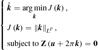 (20.77)
where Z is the Left Null Space matrix associated with ![]() . The null-space approach is characterized by the desirable feature of being an approach in which the degree and the typology of redundancy of the measured interferometric phase variations (double differences) shall not follow any specific constraint, such as the triangulation scheme in the baseline domain used in [122] that imposes a critical constraint on the generation of interferograms. This characteristic allow to freely generate the set of interferograms.
. The null-space approach is characterized by the desirable feature of being an approach in which the degree and the typology of redundancy of the measured interferometric phase variations (double differences) shall not follow any specific constraint, such as the triangulation scheme in the baseline domain used in [122] that imposes a critical constraint on the generation of interferograms. This characteristic allow to freely generate the set of interferograms.
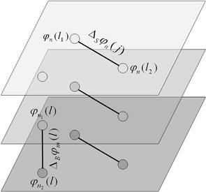
Figure 20.28 3D structure of the data corresponding to a multi-temporal multi-baseline acquisition data set: any horizontal layer corresponds to the spatial grid of a single acquisition. Vertical arcs are interferometric phase values in a pixel whereas horizontal arcs are spatial variations of interferometric phase.
2.20.6 SAR tomography
The classical SAR imaging allows high resolution capability in 2D, i.e., azimuth and range. Nevertheless, the reality is 3D and, either due to the coupling of the intrinsic side-looking geometry and the vertical structure of the targets, or to the penetration of the radiation below the imaged surface, the resulting image represents only a “projection” along the elevation direction of the illuminated 3D scene backscattering properties over the azimuth slant-range plane.
SAR tomography aims to achieving a 3D reconstruction by using the imaging diversity along the elevation direction (orthogonal to the azimuth and range plane) of (spatial) multibaseline acquisitions. In particular, as it is difficult and economically disadvantageous using several satellites to provide multibaseline acquisitions from spaceborne, SAR Tomography is typically implemented by using data corresponding to multiple passes of a single antenna SAR system over the same area. It is worth pointing out that 3D imaging capability is already available with interferometric SAR systems, relying only on the use of the phase difference between the signal acquired in at least two passes. However, InSAR implicitly assumes the presence of only a single scattering mechanism, i.e., do not comply with a possible integration (overlay) of the scattering along the elevation direction.
SAR Tomography is the extension of SAR interferometry to allow a full 3D imaging: it simply synthesize, as in the case of the azimuth direction where a array is (digitally) formed, an array also in the elevation direction by exploiting the different baselines available over repeated passes.
Most appreciable differences with respect to the azimuth synthesis is that passes are unevenly spaced in elevation and that the number of baselines is sensibly lower than the number of echoes collected in azimuth direction. The overall effect is a generally poor elevation resolution and the presence of significant distortions associated with possible excessive non-uniformity of passes.
Let us consider a multi-pass configuration exploiting N images acquired along N different orbits, not necessarily co-planar and not uniformly-spaced (see Figure 20.29). We denote with ![]() denote the nth orbit locations,
denote the nth orbit locations, ![]() , n = 1,…,N the orthogonal baselines of the nth orbit measured with respect a reference “master” orbit (
, n = 1,…,N the orthogonal baselines of the nth orbit measured with respect a reference “master” orbit (![]() in Figure 20.29), and
in Figure 20.29), and ![]() is the look angle. A ground height profile with three point scatterers (A, B, and C) lying in the same range-azimuth resolution cell is depicted.
is the look angle. A ground height profile with three point scatterers (A, B, and C) lying in the same range-azimuth resolution cell is depicted.

Letting ![]() be the signal in a fixed azimuth and range pixel at the generic nth antenna, we have [123–125]:
be the signal in a fixed azimuth and range pixel at the generic nth antenna, we have [123–125]:
![]() (20.78)
(20.78)
where ![]() (s) is the distance of the scatterer at elevation s from the nth antenna. The phase term is supposed to be not affected by APD component because the acquisitions are supposed to be simultaneous. In case of repeat pass acquisitions, the APD must be compensated. Moreover, in the latter case it is assumed that the target does not exhibit any deformation: this assumption will be relaxed for the description of the differential tomography.
(s) is the distance of the scatterer at elevation s from the nth antenna. The phase term is supposed to be not affected by APD component because the acquisitions are supposed to be simultaneous. In case of repeat pass acquisitions, the APD must be compensated. Moreover, in the latter case it is assumed that the target does not exhibit any deformation: this assumption will be relaxed for the description of the differential tomography.
The data are processed by via deramping, i.e., the distance ![]() (0) of a reference elevation point (0 in Figure 20.29) is subtracted from the data at each antenna: expanding
(0) of a reference elevation point (0 in Figure 20.29) is subtracted from the data at each antenna: expanding ![]() (0) and absorbing s-dependent terms in
(0) and absorbing s-dependent terms in ![]() (s), we have:
(s), we have:
![]() (20.79)
(20.79)
where the integral is limited to an interval of typically from few meters to hundreds of meters, and where:
![]() (20.80)
(20.80)
Equation (20.79) shows that the received data at the different antennas, in any fixed azimuth and range position, are samples of the Fourier Transform (FT) of the reflectivity function along the elevation direction at the frequencies described by Eq. (20.80), and follows the (LOS orthogonal component of) baseline distribution. SAR tomography processing aims at processing the data vector ![]() ] in such a way to achieve a reconstruction of the backscattering distribution
] in such a way to achieve a reconstruction of the backscattering distribution ![]() (s). This is carried out by inverting a discretized version of (20.79) at
(s). This is carried out by inverting a discretized version of (20.79) at ![]() elevation samples (bins)
elevation samples (bins) ![]() :
:
![]() (20.81)
(20.81)
where vector ![]() ]. Equation (20.81) provides the discrete model to be inverted in the framework of SAR tomography. Many solutions are available [124,126,127]
]. Equation (20.81) provides the discrete model to be inverted in the framework of SAR tomography. Many solutions are available [124,126,127]
2.20.6.1 Linear non-adaptive inversion for SAR tomography
A simple way to invert Eq. (20.81) and to recover the backscattering distribution is by applying the beamforming, i.e.,:
![]() (20.82)
(20.82)
that is:
![]() (20.83)
(20.83)
Note that the reconstruction of the backscattering sample ![]() is achieved via a filter
is achieved via a filter ![]() which does not depend on the data (non-adaptive inversion).
which does not depend on the data (non-adaptive inversion).
Another possibility is offered by the Singular Value Decomposition (SVD) analysis of the operator in Eq. (20.79), i.e., by the SVD decomposition of the matrix A in the discrete case. In this latter case the assumption on the support can lead to a slight degree of super-resolution with respect to the Rayleigh resolution limit for elevation, given by:
![]() (20.84)
(20.84)
where ![]() and
and ![]() are the maximum and minimum of {
are the maximum and minimum of {![]() }. The corresponding height resolution is given by:
}. The corresponding height resolution is given by:
![]() (20.85)
(20.85)
SVD decomposition provides the following fundamental equations pair:
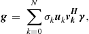 (20.86)
 (20.87)
where ![]() vector) and
vector) and ![]() vector) are the left (data) and right (unknown) singular vectors of A and
vector) are the left (data) and right (unknown) singular vectors of A and ![]() are the singular values. Note that we have assumed
are the singular values. Note that we have assumed ![]() , i.e., a sampling of the elevation interval in a number of points which is larger than the number of acquisitions thus translating in a underdetermined characteristic of the matrix A.
, i.e., a sampling of the elevation interval in a number of points which is larger than the number of acquisitions thus translating in a underdetermined characteristic of the matrix A.
Equations (20.86) and (20.87) represent the fundamental result of the SVD analysis: in particulars Eq. (20.86) states that in principle all the different vectors ![]() concur in the composition of the observed vector g; their contributions are however weighted by the singular values. Accordingly, low singular values
concur in the composition of the observed vector g; their contributions are however weighted by the singular values. Accordingly, low singular values ![]() indicates that the component along the corresponding data singular vector is attenuated by the imaging operator in the data formation and should be carefully treated when reconstructing the unknown via Eq. (20.87) because this data component may be overwhelmed by the unavoidable noise. As a result, typically the reconstruction in Eq. (20.87) is limited to the data and unknown singular vector pairs corresponding to significant singular values; the associated inversion scheme is referred to as Truncated SVD (TSVD). In the case in which the acquisitions are uniformly spaced with a separation of
indicates that the component along the corresponding data singular vector is attenuated by the imaging operator in the data formation and should be carefully treated when reconstructing the unknown via Eq. (20.87) because this data component may be overwhelmed by the unavoidable noise. As a result, typically the reconstruction in Eq. (20.87) is limited to the data and unknown singular vector pairs corresponding to significant singular values; the associated inversion scheme is referred to as Truncated SVD (TSVD). In the case in which the acquisitions are uniformly spaced with a separation of ![]() if the output sampling is chosen verifying the Nyquistic conditions, i.e.,
if the output sampling is chosen verifying the Nyquistic conditions, i.e., ![]() , i.e., N samples in the Nyquist interval
, i.e., N samples in the Nyquist interval ![]() with
with ![]() it can be shown that the operator
it can be shown that the operator ![]() in (20.81) is a Discrete Fourier Transform (DFT) matrix that is characterized by constant singular values. In such a case
in (20.81) is a Discrete Fourier Transform (DFT) matrix that is characterized by constant singular values. In such a case ![]() and therefore the direct and inverse operator in (20.86) and (20.87) becomes Hermitian conjugate pairs. In cases in which
and therefore the direct and inverse operator in (20.86) and (20.87) becomes Hermitian conjugate pairs. In cases in which ![]() the singular values shows a decay which translate the presence of a redundancy in the acquired spectral samples that can be exploited to increase the resolution of the reconstruction below the Rayleigh limit in (20.84).
the singular values shows a decay which translate the presence of a redundancy in the acquired spectral samples that can be exploited to increase the resolution of the reconstruction below the Rayleigh limit in (20.84).
In other words, by progressively restricting the elevation ROI with respect to ![]() , a smooth decay in the singular values is observed. For a reduction factor
, a smooth decay in the singular values is observed. For a reduction factor ![]() , if the noise is small enough, the truncation can be arrested to a number of singular values which is larger than FN: in this condition a degree of super resolution is achieved [124].
, if the noise is small enough, the truncation can be arrested to a number of singular values which is larger than FN: in this condition a degree of super resolution is achieved [124].
In addition to the super-resolution degree, the SVD decomposition allows also to reduce the level of sidelobes with respect to a reconstruction carried out by simple Beamforming.
2.20.6.2 Linear adaptive inversion for SAR tomography
A more general expression for the evaluation of ![]() is given by:
is given by:
![]() (20.88)
(20.88)
where ![]() is the filter for the estimation of
is the filter for the estimation of ![]() . Letting
. Letting ![]() , that is the data covariance matrix, a solution obtained mutatis mutandis from the spectral estimation theory such that:
, that is the data covariance matrix, a solution obtained mutatis mutandis from the spectral estimation theory such that:
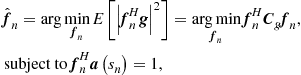 (20.89)
i.e., a solution that achieves the minimum output power, subject to unitary gain at the ‘frequency’ ![]() of interest (Capon filter), is provided by [128]:
of interest (Capon filter), is provided by [128]:
 (20.90)
Substituting (20.90) in (20.88) provides:
![]() (20.91)
(20.91)
It is interesting to note that ![]() , white data spectrum, leads to
, white data spectrum, leads to ![]() . The advantage of the Capon filer is the achievement of higher super-resolution for line spectra (i.e., concentrated scatterers along s) compared to the SVD. However a disadvantage of the Capon filter is the need to estimate the data Covariance matrix. This estimation is carried out via spatial averaging, and operation known in the SAR processing as multi-look:
. The advantage of the Capon filer is the achievement of higher super-resolution for line spectra (i.e., concentrated scatterers along s) compared to the SVD. However a disadvantage of the Capon filter is the need to estimate the data Covariance matrix. This estimation is carried out via spatial averaging, and operation known in the SAR processing as multi-look:
 (20.92)
where g(l) is the data vector in the lth pixel located close to the pixels in which the tomographic processing aims to provide an estimate of the backscattering distribution.
Note that this operation inevitably leads to a loss of azimuth-range resolution. Note also that the reconstruction of the backscattering sample ![]() is in this case data dependent (adaptive inversion).
is in this case data dependent (adaptive inversion).
An example of reconstruction of a 3D SAR image on real data is provided in Figure 20.30: in this case the results are the first one obtained by using spaceborne SAR data, specifically data acquired by the ERS sensor [124]. In the first three columns the reconstructions obtained by SVD and Capon are reported. In particular six sections in the azimuth-elevation plane (i.e., at constant slant range) of the San Paolo stadium in Naples are shows: the locations of the constant range are indicated by the horizontal white line in the last column showing the classical azimuth-range representation. It is evident the capability of the tomographic technique to capture the 3D shape of the structure. It is also evident for the Capon approach that the increase in the height resolution is paid in terms of spatial (azimuth and/or range) resolution losses.
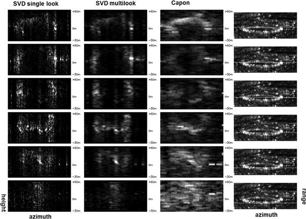
Figure 20.30 3D reconstruction of the San Paolo stadium in Naples via SVD. Left most column: elevation sections obtained by applying the SVD to the single look data. Second column: SVD with three looks. Third column Capon with five looks. In all cases the height scale is reported. Right column: azimuth range (averaged) image: the white horizontal lines indicate the position of the sections with the range.
2.20.6.3 Compressive sensing inversion for SAR tomography
A recent approach to solve the SAR tomography problem is based on Compressive Sensing [123,126,129]. Compressive Sensing CS is a model-based framework for data acquisition and signal recovery based on the premise that a signal having a sparse representation in one basis, can be reconstructed from a small number of measurements collected in a second basis, that is incoherent with the first [130]. In our case sparseness requires a small number of stable targets in the same range-azimuth resolution cell [123].
In SAR Tomography, this approaches is particularly effective [123,131] because on data acquired high frequency systems (C- or X-band sensors), the scattering in the same range-azimuth cell along the elevation occurs typically on a few concentrated scattering points, as shown in Figure 20.29.
Considering the tomographic model (20.81), the matrix A in the context of CS is called the measurement matrix [130]. As already commented before, the inversion of Eq. (20.81) is equivalent to an inverse FFT operation, and would provide an estimate of the reflectivity function with a nominal 3-dB elevation resolution given by Eq. (20.84).
In practical cases, the orbits are usually not uniformly spaced and the number N of the available acquisitions is generally much lower than the number of unknown samples ![]() . As mentioned before in Section 7.1, truncated SVD (TSVD) can be used [125] for the inversion of (20.52). An alternative technique is based on Compressive Sampling [126]. It exploits the sparsity property of the unknown vector
. As mentioned before in Section 7.1, truncated SVD (TSVD) can be used [125] for the inversion of (20.52). An alternative technique is based on Compressive Sampling [126]. It exploits the sparsity property of the unknown vector ![]() and allows obtaining very satisfactory reconstructions, even when a reduced number of acquisitions, almost randomly spaced within the overall elevation aperture, is available. Moreover, increased resolutions can be obtained adopting CS.
and allows obtaining very satisfactory reconstructions, even when a reduced number of acquisitions, almost randomly spaced within the overall elevation aperture, is available. Moreover, increased resolutions can be obtained adopting CS.
In the considered sparsity hypothesis, the sampled reflectivity function can be written as:
![]() (20.93)
(20.93)
where ![]() is the sparsity matrix and
is the sparsity matrix and ![]() is a sparse
is a sparse ![]() -dimensional vector. It has to be noted that in this case, by choosing sampling points to represent the unknown scattering distribution, and considering the circumstance that such function is sparse just in the domain of spatial samples (see also Figure 20.29, where only K = 3 scattering contributions are present in the whole scattering distribution along the elevation), the matrix
-dimensional vector. It has to be noted that in this case, by choosing sampling points to represent the unknown scattering distribution, and considering the circumstance that such function is sparse just in the domain of spatial samples (see also Figure 20.29, where only K = 3 scattering contributions are present in the whole scattering distribution along the elevation), the matrix ![]() becomes the identity matrix [123].
becomes the identity matrix [123].
An estimate of the vector ![]() can be found solving the
can be found solving the ![]() -norm minimization problem [130]:
-norm minimization problem [130]:
![]() (20.94)
(20.94)
The optimization problem in (20.94) is valid for the noiseless case. In the more realistic case, some noise is present in addition on the measurements:
![]() (20.95)
(20.95)
with w a complex Gaussian vector with zero mean and uncorrelated elements. In this case, the solution can be found by solving the linear programming problem [132]:
![]() (20.96)
(20.96)
where ![]() is a small positive number.
is a small positive number.
For discussing the super resolution issue, we can refer to the case of high signal to noise ratio, so that the maximum resolution that can be achieved depends only on the acquisition configuration and not on the noise level. The presence of an higher noise level can only degrade the evaluated performance.
In practical cases ![]() , so that Eq. (20.81) expresses an underdetermined system, which will admit a not-unique solution. Anyway, CS theory [130,132] ensures that if it is satisfied an incoherency property between A and
, so that Eq. (20.81) expresses an underdetermined system, which will admit a not-unique solution. Anyway, CS theory [130,132] ensures that if it is satisfied an incoherency property between A and ![]() , it is indeed possible to recover the K largest components
, it is indeed possible to recover the K largest components ![]() of
of ![]() from the N measurements provided that the following inequality is satisfied:
from the N measurements provided that the following inequality is satisfied:
![]() (20.97)
(20.97)
where C is a small constant depending on the measurement and sparsity matrixes A and ![]() , which can be empirically estimated by numerical simulations, K denotes the number of non-zero coefficients of
, which can be empirically estimated by numerical simulations, K denotes the number of non-zero coefficients of ![]() , and
, and ![]() is the mutual coherence between the measurement basis A and the representation (sparsity) basis
is the mutual coherence between the measurement basis A and the representation (sparsity) basis ![]() , defined in Ref. [132].
, defined in Ref. [132].
As far as the improvement or resolution, in Ref. [133] it has been shown that the elevation resolution (null-to-null) which can be obtained adopting a CS approach is given by:
![]() (20.98)
(20.98)
where ![]() is the standard Fourier techniques elevation resolution and
is the standard Fourier techniques elevation resolution and ![]() is the super-resolution factor (greater than one).
is the super-resolution factor (greater than one).
For a fixed number of acquisitions N, extension of illuminated scene in the elevation direction S, a number of scatterers K, and for a given standard resolution ![]() , there is an upper limit for the super-resolution factor given by [133]:
, there is an upper limit for the super-resolution factor given by [133]:
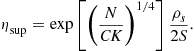 (20.99)
Combining Eqs. (20.98) and (20.99), a limit to the maximum resolution can be expressed as:
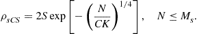 (20.100)
Equations (20.99) and (20.100) provide the super-resolution limits of the CS approach applied to SAR tomography.
Some experiments about the performance of the Compressive Sensing approach to solve the tomographic problem in terms of resolution capabilities, are presented in Ref. [123], with reference to simulated data using COSMO-Skymed system parameters (see Table 20.1), and to the real data acquired by the sensors ERS1–2, over the city of Naples, between 1998 and 2001.

The simulated observed scene is composed of two stable and coherent scatterers located in the same range-azimuth resolution cell at different elevations and responding with the same radar cross section.
In the simulation presented in Figure 20.31, it has been assumed that the SAR signals are acquired along multiple passes with a total orthogonal baseline span ![]() . The theoretical resolution in the elevation direction is given, according to Eq. (20.84), by
. The theoretical resolution in the elevation direction is given, according to Eq. (20.84), by ![]() . Assuming that the elevation extension of the ground scene is S = 200 m, the orbit spacing in the elevation direction corresponding to the Nyquist sampling rate is equal to 52 m [133].
. Assuming that the elevation extension of the ground scene is S = 200 m, the orbit spacing in the elevation direction corresponding to the Nyquist sampling rate is equal to 52 m [133].
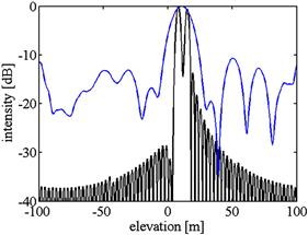
Figure 20.31 TCS interpolated and normalized reflectivity profile (black) of two scatterers at ![]() and
and ![]() obtained from nine orbits with
obtained from nine orbits with ![]() , compared with the TSVD reconstructed profile (blue) (For interpretation of the references to color in this figure legend, the reader is referred to the web version of this book.)
, compared with the TSVD reconstructed profile (blue) (For interpretation of the references to color in this figure legend, the reader is referred to the web version of this book.)
Two scatterers at the elevation values ![]() =7 m and
=7 m and ![]() are considered, so that they cannot be resolved using standard FFT based techniques, since their distance is below the system configuration resolution. Moreover,
are considered, so that they cannot be resolved using standard FFT based techniques, since their distance is below the system configuration resolution. Moreover,![]() orbits with orthogonal baselines −271 m, −238 m, −154 m, −68 m, 0 m, 64 m, 118 m, 209 m, 295 m, are considered, and the acquired signals have been corrupted with additive Gaussian noise, whose average power is 30 dB below the signal power.
orbits with orthogonal baselines −271 m, −238 m, −154 m, −68 m, 0 m, 64 m, 118 m, 209 m, 295 m, are considered, and the acquired signals have been corrupted with additive Gaussian noise, whose average power is 30 dB below the signal power.
The elevation profile obtained by the CS approach starting from the nine available acquisitions and with ![]() , corresponding to the upper limit for the resolution
, corresponding to the upper limit for the resolution ![]() is shown in Figure 20.3 (black line) where it is compared with the TSVD reconstruction (blue line), this latter able to achieve conventional “Fourier” resolutions.
is shown in Figure 20.3 (black line) where it is compared with the TSVD reconstruction (blue line), this latter able to achieve conventional “Fourier” resolutions.
In the real data experiment, 15 passes, whose orthogonal baselines span a total baseline ![]() , are used. The resulting theoretical 3 dB elevation resolution is
, are used. The resulting theoretical 3 dB elevation resolution is ![]() , which corresponds to a height resolution
, which corresponds to a height resolution ![]() . The tomographic processing of the four azimuth-height constant range sections, indicated with four segments in the ortophoto image shown in Figure 20.32, are focused and shown in Figure 20.33 using CS (left) and TSVD (right). For the CS reconstruction, a super-resolution factor
. The tomographic processing of the four azimuth-height constant range sections, indicated with four segments in the ortophoto image shown in Figure 20.32, are focused and shown in Figure 20.33 using CS (left) and TSVD (right). For the CS reconstruction, a super-resolution factor ![]() , corresponding to elevation and height resolutions of 8.87 m and 3.49 m, has been assumed. Also in this case, the sections of the San Paolo stadium in Naples in elevation (i.e., at constant slant range) shows, at different slant ranges, the capability of the technique to capture the 3D shape of the structure. A resolution improvement of the CS method with respect to the TSVD one is evident.
, corresponding to elevation and height resolutions of 8.87 m and 3.49 m, has been assumed. Also in this case, the sections of the San Paolo stadium in Naples in elevation (i.e., at constant slant range) shows, at different slant ranges, the capability of the technique to capture the 3D shape of the structure. A resolution improvement of the CS method with respect to the TSVD one is evident.
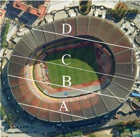
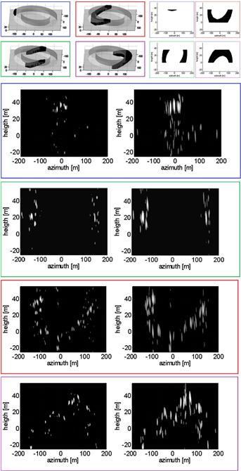
Figure 20.33 Azimuth height sections of tomographic reconstruction over the San Paolo stadium in Naples (ITALY), obtained with TCS (left) and TSVD (right). (Blue) section A, (Red) section B, (Green) section C, (Purple) section D of Figure 20.32. Credit: Univ. Napoli Parthenope; © IEEE. (For interpretation of the references to color in this figure legend, the reader is referred to the web version of this book.)
2.20.6.4 Performance comparison of SAR tomography methods
In the previous sections four SAR tomography approaches were described: Beamforming and TSVD, which attain an elevation resolution related and limited by the overall baseline span (see Eq. (20.84)), Capon, which allows super-resolution along the elevation direction, but requires the use of looks and therefore a loss of resolution, and Compressive Sensing based techniques, which exploits the sparsity of the scattering profile in elevation, and allows a strong improvement in elevation resolution.
The four method are compared with a data set simulating an observed scene composed by three stable and coherent scatterers, located in the same range-azimuth resolution cell at different elevations, and responding with the same radar cross section. More precisely the three scatterers are located at the height values ![]() ,
, ![]() , and
, and ![]() .
.
In the simulation presented in Figure 20.34, it has been assumed that the SAR signals are acquired along 30 multiple passes with a total orthogonal baseline span (![]() and therefore a mean baseline separation of 36.7 m: such a baseline distribution has been selected according to a real dataset of the Envisat satellite. According to Eq. (20.84), the theoretical resolution in the elevation direction is given by
and therefore a mean baseline separation of 36.7 m: such a baseline distribution has been selected according to a real dataset of the Envisat satellite. According to Eq. (20.84), the theoretical resolution in the elevation direction is given by ![]() , corresponding to a height resolution
, corresponding to a height resolution ![]() . The three targets have been therefore located in two resolution cells (in eleation). A total of 15 independent looks have been generated by superimposing to the complex scatterer reflectivity a uniform phase independent from look to look. Moreover, the acquired signals have been corrupted with additive Gaussian noise, whose average power is 10 dB below the signal power.
. The three targets have been therefore located in two resolution cells (in eleation). A total of 15 independent looks have been generated by superimposing to the complex scatterer reflectivity a uniform phase independent from look to look. Moreover, the acquired signals have been corrupted with additive Gaussian noise, whose average power is 10 dB below the signal power.

Figure 20.34 Results of SAR tomography on simulated data. (a) Reconstructions obtained by Beamforming, SVD and Compressive Sensing on single look data. (b) Results of Beamforming, SVD and Capon for multilook data.
The elevation interval 2a corresponding to the mean baseline is 645 m: this interval has been restricted with a reduction factor given by ![]() , thus leading to an investigated interval of 215 m.
, thus leading to an investigated interval of 215 m.
The reconstruction of the height profile obtained by the CS, SVD and Beamforming tomographic approaches, starting from the 30 available acquisitions have been generated separately for all the available looks. The result for a particular look are shown in Figure 20.34a; all approaches are able to recover correctly the presence of three scatterer present in the profile and to resolve them from each other although the super-resolution capability of the CS based approach appear to be very evident. Due to the particular realization of the noise the scatterers separation is slightly overestimated and therefore the three targets are easily visible also from the Beamforming and SVD algorithms: the latter has slightly better performances on the resolution and on the sidelobe ratio.
Beamforming, SVD, and Capon were applied to the multilook data: the result are shown in Figure 20.34b. On one hand it is evident that on average the Beamforming and SVD are not able to resolve the scatterers, although the SVD provide generally better performances with respect to the Beamforming, particularly on the sidelobe ratio. On the other hand, it is evident that in this case the Capon provide better resolution capability with respect to the other two processing approaches, by resolving the presence of the three distinct scatterers which are also located at the three correct heights. In any case differently from the CS the super-resolution degree is paid by the necessity to have different looks. A more detailed analysis of the performances of the CS tomography in terms of resolution degree can be found in [129].
2.20.7 4D Imaging
The 3D SAR focusing technique, also known as SAR Tomography allows to profile the scattering distribution along the elevation direction. Differential SAR Tomography, also referred to as 4D (3D space ![]() velocity) SAR imaging (focusing) is a natural extension of SAR Tomography to targets that exhibit displacements. It allows measuring the scattering distribution in an elevation–velocity (EV) plane, also known as tomo-doppler plane: locations of peaks in the EV plane allows identifying and measuring elevation and velocity of scatterers, even interfering in the same resolution cell. The original idea in [134] is framed in the statistical context and makes use of multilook data to estimate the data covariance matrix and then to apply adaptive (non-linear) estimation, namely Capon filtering to achieve superresolution and sidelobe reduction.
velocity) SAR imaging (focusing) is a natural extension of SAR Tomography to targets that exhibit displacements. It allows measuring the scattering distribution in an elevation–velocity (EV) plane, also known as tomo-doppler plane: locations of peaks in the EV plane allows identifying and measuring elevation and velocity of scatterers, even interfering in the same resolution cell. The original idea in [134] is framed in the statistical context and makes use of multilook data to estimate the data covariance matrix and then to apply adaptive (non-linear) estimation, namely Capon filtering to achieve superresolution and sidelobe reduction.
Again referring to 0 (the deramping reference point) we let the scatterer located at elevation s to have a deformation in the line of sight equal to ![]() , much smaller than the resolution cell; accordingly, in place of Eq. (20.79) we have the following direct model for the signal collected at the generic antenna following the deramping step:
, much smaller than the resolution cell; accordingly, in place of Eq. (20.79) we have the following direct model for the signal collected at the generic antenna following the deramping step:
![]() (20.101)
(20.101)
Moreover, the Fourier expansion of the second exponential term with respect to ![]() provides [114]:
provides [114]:
![]() (20.102)
(20.102)
with:
![]() (20.103)
(20.103)
Accordingly, Eq. (20.101) becomes:
![]() (20.104)
(20.104)
where ![]() .
.
Equation (20.104) shows that the received data are samples of the 2D Fourier Transform of the scattering distribution in the EV plane: as in the 3D case it can be inverted to estimate the backscattering distribution in the EV plane.
It is worth to note that, according to Eq. (20.102), v assumes the meaning of a spectral velocity. In analogy to the concept of instantaneous and spectral frequency in frequency modulation, there is strictly speaking no relation between v and the instantaneous temporal velocity. An exception is represented by the case in which the targets exhibit a linear temporal deformation; in this case instantaneous and spectral velocities are equal. However, under quite general conditions [135] the spectral support and the instantaneous frequency variation interval turn out to be equal. Accordingly, the appearance of focused energy in v in the elevation-velocity plane indicates the presence of scatterers with regular phase variation that can be exploited to monitor the scatterer.
MultiD (3D and 4D) focusing technique relies on the assumption that the data stack is accurately calibrated in amplitude and phase. While amplitude calibration can be easily carried out either via the use of auxiliary information provided with the data, or via simple equalization of the power on selected uniform areas or stable strong scatterers; phase calibration may be a much more complex issue due to the presence of decorrelation phenomena, APD variation and non linear deformation: the latter allows higher focusing of peaks corresponding to persistent scatterers in the EV plane.
The phase calibration step, designed to remove the atmospheric phase and low resolution (background) deformation from the signal data stack, a easy solution is by using a low resolution (small scale) processing with SBAS based interferometry approaches, to estimate and compensate for APD variation and possible non linear deformation.
Finally, a key problem associated with Multi-D imaging is the detection of scatterers that maintain persistent scattering characteristics over the time. Following the key idea of the Persistent Scatterers (PS) technique, in classical PSI techniques this step is carried out in a sequence of two stages. In the first the so called Persistent Scatterers Candidates [99,100] are selected by analyzing the stability of the amplitude response, i.e., by up-threshold, in each pixel, of the ratio between the standard deviation and the mean of the amplitude response, named amplitude dispersion index:
 (20.105)
The amplitude dispersion index is close to zero over targets showing a high stable backscattering and is proxy of the phase stability. PSC are used in PSI techniques to carry the phase calibration of the data, i.e., the estimation and removal of the Atmospheric Phase Delay (APD) contribution. In the second step, the detection of Persistent Scatterers is refined by down-threshold of the temporal coherence index in Eq. (20.68): all pixels that show a temporal coherence above the threshold are selected as PS and topography and motion parameters are provided.
In Multi-D SAR imaging the amplitude information is directly involved in the formation of the elevation profile (3D imaging) or elevation-velocity image. As far as dominant scatterers are concerned, a detector (the Generalized Maximum Likelihood Ratio Test, briefly GLRT) [136] which is derived from an optimal detection scheme (the Neuman-Pearson criterion) which maximizes the detection probability for a fixed false alarm probability is provided by [137]:
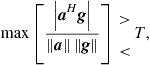 (20.106)
where the maximum has to be considered over s for the 3D case, or (s,v) for the 4D case, and T is a threshold belonging to the interval (0,1), set accordingly to the desired false alarm probability.
It is instructive to note that in the PS case, the test is obtained by letting ![]() , i.e., by eliminating from the data the amplitude information. It has been shown that, for a fixed false alarm probability, the tomographic based test allows achieving typically a gain of 1 dB in the detection of dominant scatterers [137]. Note that Eq. (20.105) is based on the selection of the peaks of the (normalized) tomographic response (
, i.e., by eliminating from the data the amplitude information. It has been shown that, for a fixed false alarm probability, the tomographic based test allows achieving typically a gain of 1 dB in the detection of dominant scatterers [137]. Note that Eq. (20.105) is based on the selection of the peaks of the (normalized) tomographic response (![]() for 3D,
for 3D, ![]() for 4D) achieved by simply applying a beamforming inversion scheme, i.e., by multiplying by the data by the transpose conjugate the direct matrix.
for 4D) achieved by simply applying a beamforming inversion scheme, i.e., by multiplying by the data by the transpose conjugate the direct matrix.
Also in terms of accuracy of the estimated mean deformation velocity and residual topography contributions the adoption of the detection scheme based on tomographic processing provides improvements. In Figure 20.35 it is shown a comparison, in terms of scatter plot of the estimated elevation for a tomographic processing (top) and for a PSI estimation.

Figure 20.35 Scatter plots of the Tomographic (top) and PSI-based (bottom) stimators for mean deformation velocity and topography for different values of the SNR.
Further studies have been carried out for the development of detections schemes able to perform a higher order analysis to detect and separate the contribution of scatterers interfering in the same resolution cell [138–141].
An example of the results obtained via 4D imaging are shown in Figure 20.36: in this case the dataset was acquired by the ERS sensor the city of over Rome. All detected single and double scatterers where geolocalized: due to the geolocalization process, scatterers located at different elevations and interfering in the same azimuth-range pixels are projected at two different ground positions, see Figure 20.37.
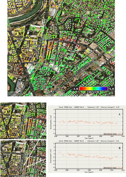
Figure 20.36 Example of separation of scatterers interfering in the same azimuth range pixel via multi-dimensional imaging and determination of velocity and time series. Top image: estimated velocity of dominant scatterers in the area of Rome. Bottom left: zoom on in an area exhibiting deformation due to alluvial deposits of the Tevere river: representation of dominant (upper image) and double (down image) scatterers. Right images: time series extracted by the double scatterers analysis.
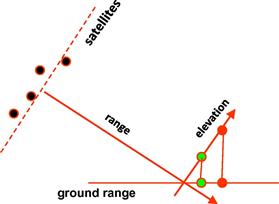
Figure 20.37 Graphical explanation of the mechanism of projection onto the ground range showing that two different scatterers located at the same range and resolved by the tomographic technique are located at different positions.
The detected single scatters (shown in the uppermost image) show the presence of deformations affecting the downtown of Rome [142]. In the two images on the left, a zoom on the results of single and double scatterers are shown to demonstrate the capability of the detected double scatterers in 4D imaging to provide important information in an area were layover impacts the monitoring capabilities, see the railway tracks. The right plots shows the capability of 4D imaging to separate time series from interfering scatterers.
Even when only a dominant scattering mechanism, it has been shown that the use of both amplitude and phase information in MDI allows to improve the performance in terms of dominant persistent scatterers detection with respect to classical PSI that uses only phase information [137].
In the following the result of a MDI processing of a set of 25 TerraSAR-X (TSX) spotlight data acquired over ascending orbits over the city of Las Vegas, Nevada, USA is shown [19]: in this case the improvement of resolution from ![]() of ERS to
of ERS to ![]() of TerraSAR-X makes the layover of buildings much more evident.
of TerraSAR-X makes the layover of buildings much more evident.
In particular, in Figure 20.38 it is shown the reconstruction of the Mirage Hotel obtained by detecting persistent scatterers on a 1st order (single scatterers) and 2nd order (double scatterers interfering in the same pixel) analysis. The possibility to synthesize a fine beam also in the elevation direction provide the TerraSAR-X sensor with the capability of reconstructing the building in 3D. In Figure 20.39 it is shown the result of the multidimensional analysis, specifically the topography for the single and double scatterers: the mid and right images shows the capability of the tomographic based processing of solving the layover and hence separating the contribution of the two layers of the ground and façade interfering due to the mechanism of folding of the vertical building toward the left (near range). The measured deformations show essentially only the presence of thermal dilations for the roof area. Another example of the effectiveness of multi-dimensional imaging is provided in Figure 20.40 for the Bellagio hotel. The image on the right shows the final set of detected single and double scatterers and the results, especially on the upper façade of the building where interference with the ground is much critical, shows a significant improvement in the reconstruction of the building structure.
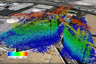
Figure 20.38 Example of reconstruction at full resolution of the Mirage Hotel in Las Vegas, USA obtained by processing 1 m resolution spotlight data with a 4D imaging approach. Credit IREA-CNR and DLR, © IEEE.

Figure 20.39 Detected scatterers for the formation of image in Figure 20.38. From left to right, single scatterers, lower layer of double scatterers and top layer of double scatterers. Credit IREA-CNR and DLR, © IEEE.
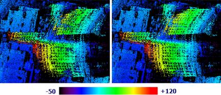
2.20.8 Conclusion
This review work has addressed the topics related to SAR interferometry and SAR Tomography. For the first topic we have described in details both from a deterministic and stochastic viewpoint the single and multibaseline interferometric technique for the estimation of the topographic height. Furthermore, the differential interferometry technique has been addressed for the description of the possibility to accurately monitor small deformation of the Earth surface, especially with reference to the application to volcanic and seismic risk. Persistent scatterers interferometry, the differential interferometry technique that has for the first time shown the possibility to accurately monitor deformation, finds it “killer application” to monitoring of man-made structures and has been also addressed. Furthermore whole sections have been devoted to SAR tomography, also known as multi-dimensional imaging, which is a technique based on an imaging approach and extends the concepts of interferometry. By using the amplitude and phase information collected over multi-baseline multipass data it provides the best technology currently used for the imaging and monitoring of urban areas and infrastructures. SAR tomography is also applied for volume scattering profiling with application to forest mapping [125], particularly in conjunction with polarimetry with a technique known as Polarimetric SAR Tomography. In this review work we have limited our analysis to surface scattering single polarization: Further description of SAR Tomography and Polarimetric SAR tomography can be found in [21,22,143]. Finally application examples including results obtained with the recent very high resolution SAR sensors have been provided to give the reader the possibility to have information about the current applicability, potential and limits of the coherent SAR processing.
References
1. Moreira A, Prats-Iraola P, Younis M, Krieger G, Hajnsek I, Papathanassiou KP. A tutorial on synthetic aperture radar. IEEE Geosci Rem Sens Mag. 2013;1(1):6–43.
2. Wiley CA. Synthetic aperture radars: a paradigm for technology evolution. IEEE Trans Aerosp Electron Syst. 1985;21(3):440–443.
3. Bamler R, Hartl P. Synthetic aperture radar interferometry. Inverse Probl. 1998;14:R1–R54.
4. Rosen PA, Hensley S, Joughin IR, et al. Synthetic aperture radar interferometry. Proc IEEE. 2000;88(3):333–382.
5. Romeiser R, Breit H, Eineder M, et al. Current measurements by SAR along-track interferometry from a Space Shuttle. IEEE Trans Geosci Remote Sens. 1995;43(10):2315–2324.
6. ERS. <https://earth.esa.int/web/guest/missions/esa-operational-eo-missions/ers>.
7. CSK. <http://www.asi.it/en/activity/earth_observation/cosmoskymed>.
8. TerraSAR. Available from:<http://www.dlr.de/dlr/en/desktopdefault.aspx/tabid-10377/565_read-436/>.
9. Lee JS, Pottier E. Polarimetric Radar Imaging: From Basics to Applications. CRC Press 2009.
10. Cloude SR, Pottier E. A review of target decomposition theorems in radar polarimetry. IEEE Trans Geosci Remote Sens. 1996;34(2):498–518.
11. Cloude SR, Pottier E. An entropy-based classification scheme for land applications of polarimetric SAR. IEEE Trans Geosci Remote Sens. 1997;35(1):68–78.
12. Freeman A, Durden ST. A three-component scattering model for polarimetric SAR data. IEEE Trans Geosci Remote Sens. 1998;36(3):963–973.
13. Touzi R, Boerner WM, Lee JS, Lueneburg E. A review of polarimetry in the context of synthetic aperture radar: concepts and information extraction. Can J Remote Sens. 2004;30(3):380–407.
14. Le Toan T, Beaudoin A, Guyon D. Relating forest biomass to SAR data. IEEE Trans Geosci Remote Sens. 1992;30(2):403–411.
15. Hajnsek I, Pottier E, Claude S. Inversion of surface parameters from polarimetric SAR. IEEE Trans Geosci Remote Sens. 2003;41(4):727–744.
16. Hajnsek I, Jagdhuber T, Shon H, Papathanassiou KP. Potential of estimating soil moisture under vegetation cover by means of PolSAR. IEEE Trans Geosci Remote Sens. 2009;42(2):442–454.
17. Cloude SR, Papathanassiou K. Polarimetric SAR interferometry. IEEE Trans Geosci Remote Sens. 1998;36(4):1551–1565.
18. Papathanassiou KP, Cloude SR. Single-baseline polarimetric SAR interferometry. IEEE Trans Geosci Remote Sens. 2001;39(6):2352–2363.
19. Reale D, Fornaro G, Pauciullo A, Zhu X, Bamler R. Tomographic imaging and monitoring of buildings with very high resolution SAR data. IEEE Geosci Remote Sens Lett. 2011;8(4):661–665.
20. Fornaro G, Pauciullo A, Reale D, Zhu X, Bamler R. SAR tomography: an advanced tool for 4D spaceborne radar scanning with application to imaging and monitoring of cities and single Buildings. IEEE Geosci Remote Sens Newslett. 2012;10–18.
21. Tebaldini S. Single and multipolarimetric SAR tomography of forested areas: a parametric approach. IEEE Trans Geosci Remote Sens. 2010;48(5):2375–2387.
22. Tebaldini S, Rocca F. Multibaseline polarimetric SAR tomography of a boreal forest at P- and L-Bands. IEEE Trans Geosci Remote Sens. 2012;50(1):232–246.
23. Cloude SR. Polarization coherence tomography. Radio Sci. 2006;41. doi 10.1029/2005RS003436.
24. Cloude SR. Dual-baseline coherence tomography. IEEE Geosci Remote Sens Lett. 2007;4(1):127–131.
25. Curlander JC, McDonough RN. Synthetic Aperture Radar: Systems and Signal Processing. Wiley-Interscience 1991.
26. Elachi C. Spaceborne Radar Remote Sensing: Applications and Techniques. IEE 1988.
27. Ducoff MR, Titjen BW. Pulse Compression Radar. In: Skolnik M, ed. Radar Handbook. third ed. McGraw-Hill Professional 2008; (Chapter 8).
28. Cumming IG, Wong FH. Digital Processing of Synthetic Aperture Radar Data: Algorithms And Implementation. Artech House Remote Sensing Library 2005.
29. Carrara WG, Majewski RM, Goodman RS. Spotlight Synthetic Aperture Radar: Signal Processing Algorithms. Artech House Remote Sensing Library 1995.
30. Mittermayer L, Moreira A, Loffeld O. Spotlight SAR data processing using the frequency scaling algorithm. IEEE Trans Geosci Remote Sens. 1999;37(5):2198–2214.
31. Prats P, Scheiber R, Mittermayer J, Meta A, Moreira A. Processing of sliding spotlight and TOPS SAR data using baseband azimuth scaling. IEEE Trans Geosci Remote Sens. 2010;48(2):770–780.
32. Lanari R, Zoffoli S, Sansosti E, Fornaro G, Serafino F. A new approach for hybrid stripmap/spotlight SAR data focusing. IEE Proc Radar Sonar Navig. 2001;148:363–372.
33. Bamler R, Eineider M. ScanSAR processing using standard high precision SAR algorithms. IEEE Trans Geosci Remote Sens. 1996;34(1):212–218.
34. De Zan F, Monti Guarnieri A. TOPSAR: Terrain observation by progressive scans. IEEE Trans Geosci Remote Sens. 2006;44(9):2352–2360.
35. Eineder M, Adam N, Bamler R, Yague-Martinez N, Breit H. Spaceborne spotlight SAR interferometry with terraSAR-X. IEEE Trans Geosci Remote Sens. 2009;47(5):1524–1535.
36. Ulaby FT, Moore RK, Fung A. Microwave Remote Sensing: Active and Passive, Radar Remote Sensing and Surface Scattering and Emission Theory. vol. II Artech House Publishers 1986.
37. Franceschetti G, Fornaro G. Synthetic aperture radar interferometry. In: Franceschetti G, Lanari R, eds. Synthetic Aperture Radar Processing. CRC Press 1999;167–223.
38. Gabriel AK, Goldstein RM. Crossed orbit interferometry: theory and experimental results from SIR-B. Int J Remote Sens. 1988;9:857–872.
39. Rodriguez E, Martin JM. Theory and design of interferometric synthetic aperture radars. Proc Inst Elect Eng Part F. 1992;139:147–159.
40. Ferretti A, Prati C, Rocca F. Multibaseline DEM reconstruction: the wavelet approach. IEEE Trans Geosci Remote Sens. 1999;37:705–715.
41. Lombardini F. Optimum absolute phase retrieval in a three-element SAR interferometer. Electron Lett. 1998;34:1522–1524.
42. Pascazio V, Schirinzi G. Estimation of terrain elevation by multi-frequency interferometric wide band SAR Data. IEEE Signal Process Lett. 2001;8:7–9.
43. Goldstein RM, Zebker HA. Interferometric radar measurements of ocean surface currents. Nature 1987;707–709.
44. Romeiser R, Breit H, Eineder M, et al. Current measurements by SAR along-track interferometry from a space shuttle. IEEE Trans Geosci Remote Sens. 2005;43(10):2315–2324.
45. Budillon A, Pascazio V, Schirinzi G. Estimation of radial velocity of moving targets by along-track interferometric SAR systems. IEEE Geosci Rem Sens Lett. 2008;5(3):349–353.
46. Budillon A, Pascazio V, Schirinzi G. Multi-channel along-track interferometric SAR systems: moving targets detection and velocity estimation. Int J Navig Obs. 2008;Q3:1–16.
47. Franceschetti G, Lanari R, Pascazio V, Schirinzi G. WASAR: a Wide angle SAR processor. IEE Proc F. 1992;139(2):107–114.
48. Graham LC. Synthetic interferometer for topographic mapping. Proc IEEE. 1974;62:763–768.
49. Hellwick O, Ebner H. Geocoding SAR interferograms by least squares adjustment. J Photogramm Remote Sens. 2000;55(4):277–288.
50. Van Zyl JJ. The shuttle radar topography mission (SRTM): a breakthrough in remote sensing of topography. Acta Astronaut. 2001;48(5–12):559–565.
51. Krieger G, Moreira A, Fiedler H, et al. TanDEM-X: a satellite formation for high-resolution SAR interferometry. IEEE Trans Geosci Remote Sens. 2007;45(11):3317–3341.
52. Lucido M, Meglio F, Pascazio V, Schirinzi G. Closed form evaluation of the second order statistical distribution of the interferometric phases in dual-baseline SAR systems. IEEE Trans Signal Proc. 2010;58(3):1698–1707.
53. Just D, Bamler R. phase statistics of interferograms with applications to synthetic aperture radar. App Opt. 1994;33(20):4361–4368.
54. Fornaro G, Franceschetti G. Image registration in interferometric SAR processing. IEE Proc Radar Sonar Navig. 1995;142:313–320.
55. Gatelli F, Monti Guarnieri A, Parizzi F, Pasquali P, Prati C, Rocca F. The wave-number shift in SAR interferometry. IEEE Trans Geosci Remote Sens. 1994;32:855–865.
56. Ferraiuolo G, Meglio F, Pascazio V, Schirinzi G. DEM reconstruction accuracy in multi-channel SAR interferometry. IEEE Trans Geosci Rem Sens. 2009;47(1):191–201.
57. Zebker SHA, Villasenor J. Decorrelation in interferometric radar echoes. IEEE Trans Geosci Remote Sens. 1992;30:950–959.
58. Chen CW, Zebker HA. Two-dimensional phase unwrapping with use of statistical models for cost functions in nonlinear optimization. J Opt Soc Am A. 2001;18:338–351.
59. Chen CW, Zebker HA. Phase unwrapping for large SAR interferograms: statistical segmentation and generalized network models. IEEE Trans Geosci Remote Sens. 2002;40(8):1709–1719.
60. Costantini M. A novel phase unwrapping method based on network programming. IEEE Trans Geosci Remote Sens. 1998;36(3):813–821.
61. Fornaro G, Franceschetti G, Lanari R. Interferometric SAR phase unwrapping using Green’s formulation. IEEE Trans Geosci Remote Sens. 1996;34(3):720–727.
62. Ghiglia DC, Romero LA. Robust two-dimensional weighted and unweighted phase unwrapping that uses fast transforms and iterative methods. J Opt Soc Amer A. 1994;11(1):107–117.
63. Goldstein RM, Zebker HA, Werner CL. Satellite radar interferometry: two-dimensional phase unwrapping. Radio Sci. 1998;23(4):713–720.
64. Proakis JG, Salehi M. Communication Systems Engineering. second ed. Prentice Hall 2001.
65. Davenport WB, Root WL. An Introduction to the Theory of Random Signal and Noise. IEEE Communications Society Press 1987.
66. Prati C, Rocca F. Improving Slant-Range Resolution with Multiple SAR Surveys. IEEE Trans, Aerosp Electron Syst. 1993;29:135–144.
67. Fornaro G, Guarnieri Monti A. Minimum mean square error space-varying filtering of interferometric SAR data. IEEE Trans Geosci Remote Sens. 2002;40:11–21.
68. Goldstein RM, Engelhardt H, Kamb B, Froclich RM. Satellite RADAR interferometry for monitoring ice-sheet motion—application to an Antarctic ice stream. Science. 1993;262(5139):1525–1530.
69. Massonnet D, Rossi M, Carmona C, et al. The displacement field of the Landers earthquake mapped by radar interferometry. Nature. 1993;364(6433):138–142.
70. Peltzer G, Rosen PA. Surface displacement of the 17 May 1993 Eureka valley, California, Earthquake observed by SAR interferometry. Science. 1995;268:1333–1336.
71. Lanari R, Lundgren P, Sansosti E. Dynamic deformation of etna volcano observed by satellite radar interferometry. Geophy Res Lett. 1998;25(10):1541–1544.
72. Massonnet D, Briole P, Arnaud A. Deflation of Mount Etna monitored by spaceborne radar interferometry. Nature. 1995;375:567–570.
73. Rignot E. Fast recession of a west antartic glacier. Science. 1998;281:549–551.
74. Hanssen RF. Radar Interferometry: Data Interpretation and Error Analysis (Remote Sensing and Digital Image Processing). Springer 2001.
75. Goldsteing RM, Zebker HA, Werner CL. Satellite radar interferometry: two dimensional phase unwrapping. Radio Sci. 1998;23(4):713–720.
76. Ghiglia DC, Pritt MD. Two-Dimensional Phase Unwrapping: Theory, Algorithms, and Software. Wiley-Interscience 1998.
77. Ghiglia DC, Romero LA. Minimum ![]() -norm two-dimensional phase unwrapping. J Opt Soc Amer A. 1996;13:1999–2007.
-norm two-dimensional phase unwrapping. J Opt Soc Amer A. 1996;13:1999–2007.
78. Flynn TJ. Two-dimensional phase unwrapping with minimum weighted discontinuity. J Opt Soc Am A. 1997;14:2692–2701.
79. Costantini M, Rosen PA. A Generalized Phase Unwrapping Approach for Sparse Data. In: Proc Int Geosci Remote Sens Symp (IGARSS 1999) Hamburg, Germany. 1999;267–269.
80. Bamler R, Eineider M. Accuracy of differential shift estimation by correlation and split-bandwidth interferometry for wideband and delta-k SAR systems. IEEE Geosci Remote Sens Lett. 2005;2(2):151–155.
81. Fornaro G, Pauciullo A, Sansosti E. Phase difference-based multichannel phase unwrapping. IEEE Trans Image Proc. 2005;14:960–972.
82. Fornaro G, Monti Guarnieri A, Pauciullo A, De-Zan F. Maximum likelihood multi-baseline SAR interferometry. IEE Proc Radar Sonar Navigat. 2006;153:279–288.
83. Pascazio V, Schirinzi G. Multi-frequency InSAR height reconstruction through maximum likelihood estimation of local planes parameters. IEEE Trans Image Process. 2002;11:1478–1489.
84. Xu W, Chang E, Kwoh L, Lim H, Cheng W. Phase-unwrapping of SAR interferogram with multi-frequency or multi-baseline. In: Proc Int Geosci Remote Sens Symp (IGARSS 1994), Pasadena, USA. 1994;730–732.
85. Ferraioli G, Shabou A, Tupin F, Pascazio V. Multichannel phase unwrapping with graph-cuts. IEEE Geosci Remote Sens Lett. 2009;6(3):562–566.
86. Dias J, Leitao J. The ![]() algorithm: a method for interferometric image reconstruction in SAR/SAS. IEEE Trans Image Process. 2002;11:408–422.
algorithm: a method for interferometric image reconstruction in SAR/SAS. IEEE Trans Image Process. 2002;11:408–422.
87. Ferraiuolo G, Pascazio V, Schirinzi G. Maximum a posteriori estimation of Height profiles in InSAR imaging. IEEE Geosci Remote Sens Lett. 2004;1:66–70.
88. Nico G, Palubinskas G, Datcu M. Bayesian approach to phase unwrapping: theoretical study. IEEE Trans Signal Process. 2000;48:2545–2556.
89. Kay SM. Fundamentals of Statistical Signal Processing: Estimation Theory. Prentice Hall 1993.
90. Li SZ. Markov Random Field Modelling in Computer Vision. Computer Science Workbench Springer 2001.
91. Geman S, Geman D. Stochastic relaxation, Gibbs’ distributions, and Bayesian restoration of images. IEEE Trans Pattern Anal Mach Intell. 1984;6:721–741.
92. Shabou A, Baselice F, Ferraioli G. Urban digital elevation model reconstruction using very high resolution multi-channel InSAR data. IEEE Trans Geosci Remote Sens. 2012;50:4748–4758.
93. Rudin LI, Osher S, Fatemi E. Nonlinear total variation based noise removal algorithms. Physica D. 1992;60(1–4):259–268.
94. Ishikawa H. Exact optimization for markov random fields with convex priors. IEEE Trans Pattern Anal Mach Intell. 2003;25:1333–1336.
95. Boykov Y, Veksler O, Zabih R. Fast approximate energy minimization via graph cuts. IEEE Trans Pattern Anal Mach Intell. 2001;23(11):1222–1239.
96. Kolmogorov V, Zabih R. Multi-camera scene reconstruction via graph cuts. In: 2002;82–96. Proceedings of the 7th European Conference on Computer Vision. 3.
97. Boykov Y, Kolmogorov V. An experimental comparison of min-cut/max-flow algorithms for energy minimization in vision. Energy Minimization Methods in Computer Vision and Pattern Recognition 2001;359–374.
98. Castellanos J, Gomez S, Guerra V. The triangle method for finding the corner of the L-curve. Appl Numer Math. 2002;43(4):359–373.
99. Ferretti A, Prati C, Rocca F. Nonlinear subsidence rate estimation using permanent scatterers in differential SAR interferometry. IEEE Trans Geosci Remote Sens. 2000;38:2202–2212.
100. Ferretti A, Prati C, Rocca F. Permanent scatterers in SAR interferometry. IEEE Trans Geosci Remote Sens. 2001;39(1):8–20.
101. Crosetto M, Biescas E, Duro J, Closa J, Arnaud A. Generation of advanced ERS and envisat interferometric SAR products using the stable point network technique. Photogramm Eng. 2008;74(4):443–451.
102. N. Adam, B. Kampes, M. Eineder, J. Worawattanamateekul, M. Kircher, in: The Development of a Scientific Permanent Scatterer System, ISPRS Hannover Workshop, Hannover, Germany, 2003.
103. Werner C, Wegmuller U, Strozzi T, Wiesmann A. Interferometric point target analysis for deformation mapping. In: Proc Int Geosci Remote Sens Symp., (IGARSS 2003), Toulouse, France. 2003.
104. Bovenga F, Nutricato R, Refice A, Wasowski J. Application of multi-temporal differential interferometry to slope instability detection in Urban/Peri-Urban areas. Eng Geol. 2006;88:219–240.
105. Costantini M, Falco S, Malvarosa F, Minati F, Trillo F. Method of persistent scatterers pairs (PSP) and high resolution SAR interferometry. In: Proc Int Geosci Remote Sensing Symp (IGARSS 2009), Cape Town, South Africa. 2009.
106. Hooper A, Segall P, Zebker H. Persistent scatterer InSAR for crustal deformation analysis with application to volcán Alcedo, Galàpagos. J Geophys Res. 2007;112:B07407.
107. Hilley GE, Burgmann R, Ferretti A, Novali F, Rocca F. Dynamics of Slow-Moving Landslides from Permanent Scatterer Analysis. Science. 2004;304(5679):1952–1955.
108. Herrera G, Davalillo JC, Mulas J, Cooksley G, Monserrat O, Pancioli V. Mapping and monitoring geomorphological processes in mountainous areas using PSI data: central pyrenees case study. Nat Hazard Earth Syst Sci. 2009;9:1587–1598.
109. Berardino P, Fornaro G, Lanari R, Sansosti E. A new algorithm for surface deformation monitoring based on small baseline differential SAR interferograms. IEEE Trans Geosci Remote Sens. 2002;40(11):2375–2383.
110. Blanco-Sanchez P, Mallorqui J, Duque S, Monnells D. The Coherent pixels technique (CPT): an advanced DInSAR technique for nonlinear deformation monitoring. Pure Appl Geophys. 2008;165(6):1167–1193.
111. Mora O, Mallorqui J, Broquetas A. Linear and non-linear terrain deformation maps from a reduced set of interferometric SAR images. IEEE Trans Geosci Remote Sens. 2003;41(10):2243–2253.
112. Golub GH, Van Loan CF. Matrix Computations. Johns Hopkins University Press 1996.
113. Refice A, Bovenga F, Nutricato R. MST-based stepwise connection strategies for multipass Radar data, with application to coregistration and equalization. IEEE Trans Geosci Remote Sens. 2006;44(8):2029–2040.
114. Fornaro G, Reale D, Serafino F. Four-dimensional SAR imaging for height estimation and monitoring of single and double scatterers. IEEE Trans Geosci Remote Sens. 2009;47(1):224–237.
115. Fornaro G, Pauciullo A, Serafino F. Deformation monitoring over large areas with multipass differential sar interferometry: a new approach based on the use of spatial differences. Int J Remote Sens. 2009;30(6):1455–1478.
116. D’Agostino N, Cheloni D, Fornaro G, Giuliani R, Reale D. Space-time distribution of afterslip following the 2009 L’Aquila earthquake. J Geophys Res. 2012;117:B02402. doi 10.1029/2011JB008523.
117. S. Gernhardt, R. Bamler, Deformation monitoring of single buildings using meter-resolution SAR data in PSI, ISPRS J. Photogramm. Remote Sens. (2012) (in print).
118. Touzi R, Lopes A, Bruniquel J, Vachon PW. Coherence estimation for SAR imagery. IEEE Trans Geosci Remote Sens. 1999;37:135–149.
119. Fornaro G, Pauciullo A, Reale D. A null-space method for the phase unwrapping of multi-temporal sar interferometric stacks. IEEE Trans Geosci Remote Sens. 2011;49(6):2323–2334.
120. Agram P, Zebker H. Edgelist phase unwrapping algorithm for time-series InSAR analysis. J Opt Soc Am A. 2010;27(3):605–612.
121. M. Costantini, F. Malvarosa, F. Minati, A general formulation for robust and efficient integration of finite differences and phase unwrapping on sparse multidimensional domains, in: ESA Fringe 2009 Workshop, Frascati, Italy, 2009.
122. Pepe A, Lanari L. On the extension of the minimum cost flow algorithm for phase unwrapping of multitemporal differential SAR interferograms. IEEE Trans Geosci Remote Sens. 2006;44(9):2374–2383.
123. Budillon A, Evangelista A, Schirinzi G. Three-dimensional SAR focusing from multipass signals using compressive sampling. IEEE Trans Geosci Remote Sens. 2011;49(1):488–499.
124. Fornaro G, Lombardini F, Serafino F. Three-dimensional multipass SAR focusing: experiments with long-term spaceborne data. IEEE Trans Geosci Remote Sens. 2005;43(4):702–714.
125. Reigber A, Moreira A. First demonstration of airborne SAR tomography using multibaseline L-band data. IEEE Trans Geosci Remote Sens. 2000;38(5):2142–2152.
126. Budillon A, Evangelista A, Schirinzi G. SAR Tomography from Sparse Samples. In: Proc IEEE Int Geosci Remote Sens Symp (IGARSS 2009). 2009;IV-865–IV-868.
127. Gini F, Lombardini F. Multibaseline cross-track SAR interferometry: a signal processing perspective. IEEE Aerosp Electron Sys Mag. 2005;20(8):71–93.
128. Lombardini F, Montanari M, Gini F. Reflectivity estimation for multibaseline interferometric radar imaging of layover extended sources. IEEE Trans Signal Process. 2003;51:1508–1519.
129. Zhu XX, Bamler R. Super-resolution power and robustness of compressive sensing for spectral estimation with application to spaceborne tomographic SAR. IEEE Trans Geosci Remote Sens. 2012;50(1):247–258.
130. Candes EJ, Wakin MB. An introduction to compressive sampling. IEEE Signal Process Mag. 2008;25(2):21–30.
131. Zhu XX, Bamler R. Demonstration of super-resolution for tomographic SAR imaging in urban environment. IEEE Trans Geosci Remote Sens. 2012; In: <http://dx.doi.org/10.1109/TGRS.2011.2177843>; 2012.
132. Candes EJ, Tao T. The Dantzig selector: statistical estimation when p is much larger than n. Ann Statist. 2007;35(6):2313–2351.
133. Budillon A, Schirinzi G. Artifact Reduction in SAR Compressive Sampling Tomography. In: Proc Int Geosci Remote Sens Symp 2011 (IGARSS 2011). 2011;2700–2703.
134. Lombardini F. Differential tomography: a new framework for SAR interferometry. IEEE Trans Geosci Remote Sens. 2005;43(1):37–44.
135. Carlson AB, Crilly PB. Communication Systems. fifth ed. Mc Graw Hill Higher Education 2009.
136. Kay SM. Fundamentals of Statistical Signal Processing: Detection Theory. Prentice Hall 1998.
137. De Maio A, Fornaro G, Pauciullo A. Detection of single scatterers in multdimensional SAR imaging. IEEE Trans Geosci Remote Sens. 2009;47(7):2284–2997.
138. Pauciullo A, Reale D, De Maio A, Fornaro G. Detection of double scatterers in SAR tomography. IEEE Trans Geosci Remote Sens. 2012;50(9):3567–3586.
139. Zhu X, Bamler R. Very high resolution spaceborne SAR tomography in urban environment. IEEE Trans Geosci Remote Sens. 2010;48(12):4296–4308.
140. Lombardini F, Pardini M. Multiple scatterers identification in complex scenarios with adaptive differential tomography. In: Proceedings of the International Geoscience and Remote Sensing Symposium, Cape Town, South Africa. July 2009.
141. Lombardini F, Gini F. Model order selection in multibaseline interferometric radar systems. EURASIP J Adv Signal Proc. 2005;2005(20):3206–3219.
142. Fornaro G, Serafino F, Reale D. 4-D SAR imaging: the case study of Rome. IEEE Geosci Remote Sens Lett. 2010;7:236–240.
143. Cloude SR. Dual-baseline Coherence Tomography. IEEE Geosci Remote Sens Lett. 2007;4(1):127–131.
1For interpretation of color in Figures 20.7 and 20.12 the reader is referred to the web version of this book.
2The term “absolute” is in the phase unwrapping context related to the restriction operator and does not concern the absolute value operator.