
Blind Signal Separation for Digital Communication Data
Antoine Chevreuil* and Philippe Loubaton†, *ESIEE Paris/UMR 8049 LIGM, 2 bd Blaise Pascal BP 99, 93162 Noisy-le-grand cedex, France, †Université de Paris-Est Marne-la-Vallée, UMR 8049 LIGM, 5 bd Descartes, 77454 Marne-la-Vallée cedex 2, France
Abstract
Blind source separation, often called independent component analysis, is a main field of research in signal processing since the eighties. It consists in retrieving the components, up to certain indeterminacies, of a mixture involving statistically independent signals. Solid theoretical results are known; besides, they have given rise to performance algorithms. There are numerous applications of blind source separation. In this contribution, we particularize the separation of telecommunication sources. In this context, the sources stem from telecommunication devices transmitting at the same time in a given band of frequencies. The received data is a mixed version of all these sources. The aim of the receiver is to isolate (separate) the different contributions prior to estimating the unknown parameters associated with a transmitter. The context of telecommunication signals has the particularity that the sources are not stationary but cyclo-stationary. Now, in general, the standard methods of blind source separation assume the stationarity of the sources. In this contribution, we hence make a survey of the well-known methods and show how the results extend to cyclo-stationary sources.
2.04.1 Introduction
2.04.1.1 Generalities on blind source separation
The goal of blind source separation is to retrieve the components of a mixture of independent signals when no a priori information is available on the mixing matrix. This question was introduced in the eighties in the pioneering works of Jutten and Herault [1]. Since then, Blind Source Separation (BSS), also called independent component analysis, was developed by many research teams in the context of various applicative contexts. The purpose of this chapter is to present BSS methods that have been developed in the past in the context of digital communications. In this case, K digital communication devices sharing the same band of frequencies transmit simultaneously K signals. The receiver is equipped with ![]() antennas, and has to retrieve a part of (or even all) the transmitted signals. The use of BSS techniques appears to be relevant when the receiver has no a priori knowledge on the channels between the transmitters and the receiver. As many digital communication systems use training sequences which allow one to estimate the channels at the receiver side, blind source separation is in general not a very useful tool. However, it appears to be of particular interest in contexts such as spectrum monitoring or passive listening in which it is necessary to characterize unknown transmitters (estimation of technical parameters such as the carrier frequency, symbol rate, symbol constellation,…) interfering in a certain bandwidth. For this, it is reasonable to try to firstly retrieve the transmitted signals, and then to analyze each of them in order to characterize the system it has been generated by. In this chapter, we provide a comprehensive introduction to the blind separation techniques that can be used to achieve the first step.
antennas, and has to retrieve a part of (or even all) the transmitted signals. The use of BSS techniques appears to be relevant when the receiver has no a priori knowledge on the channels between the transmitters and the receiver. As many digital communication systems use training sequences which allow one to estimate the channels at the receiver side, blind source separation is in general not a very useful tool. However, it appears to be of particular interest in contexts such as spectrum monitoring or passive listening in which it is necessary to characterize unknown transmitters (estimation of technical parameters such as the carrier frequency, symbol rate, symbol constellation,…) interfering in a certain bandwidth. For this, it is reasonable to try to firstly retrieve the transmitted signals, and then to analyze each of them in order to characterize the system it has been generated by. In this chapter, we provide a comprehensive introduction to the blind separation techniques that can be used to achieve the first step.
In order to explain the specificity of the problems we address in the following, we first recall what are the most classical BSS methodologies. The observation is a discrete-time M-variate signal ![]() defined as
defined as ![]() where the components of the K-dimensional (
where the components of the K-dimensional (![]() ) time series
) time series ![]() represent K signals which are statistically independent. The signal y is thus an instantaneous mixture of the K independent source signals
represent K signals which are statistically independent. The signal y is thus an instantaneous mixture of the K independent source signals ![]() in the sense that
in the sense that ![]() only depends on the value of s at time n. The signal y is said to be a convolutive mixture of the K independent source signals
only depends on the value of s at time n. The signal y is said to be a convolutive mixture of the K independent source signals ![]() if
if ![]() where
where ![]() represents the transfer function
represents the transfer function ![]() . For the sake of simplicity, we just consider the context of instantaneous mixtures in this introductory section. The goal of blind source separation is to retrieve the signals
. For the sake of simplicity, we just consider the context of instantaneous mixtures in this introductory section. The goal of blind source separation is to retrieve the signals ![]() from the sole knowledge of the observations. Fundamental results of Darmois (see e.g., [2]) show that if the source signals are non Gaussian, then it is possible to achieve the separation of the sources by adapting a matrix
from the sole knowledge of the observations. Fundamental results of Darmois (see e.g., [2]) show that if the source signals are non Gaussian, then it is possible to achieve the separation of the sources by adapting a matrix ![]() in such a way that the components of
in such a way that the components of ![]() are statistically independent. For this, it has been shown that it is sufficient to optimize over G a function, usually called a contrast function, that can be expressed in terms of certain moments of the joint probability distribution of
are statistically independent. For this, it has been shown that it is sufficient to optimize over G a function, usually called a contrast function, that can be expressed in terms of certain moments of the joint probability distribution of ![]() . A number of successful contrast functions have been derived in the case where the signal
. A number of successful contrast functions have been derived in the case where the signal ![]() are stationary sequences [2–5]. However, it will be explained below that in the context of digital communications, the signals
are stationary sequences [2–5]. However, it will be explained below that in the context of digital communications, the signals ![]() are not stationary, but cyclostationary, in the sense that their statistical properties are almost periodic function of the time index. For example, for each k, the sequence
are not stationary, but cyclostationary, in the sense that their statistical properties are almost periodic function of the time index. For example, for each k, the sequence ![]() appears to be a superposition of sinusoids whose frequencies, called cyclic frequencies, depend on the symbol rate of transmitter k, and are therefore unknown at the receiver side. The cyclostationarity of the
appears to be a superposition of sinusoids whose frequencies, called cyclic frequencies, depend on the symbol rate of transmitter k, and are therefore unknown at the receiver side. The cyclostationarity of the ![]() induces specific methodological difficulties that are not relevant in other applications of blind source separation.
induces specific methodological difficulties that are not relevant in other applications of blind source separation.
2.04.1.2 Illustration of the potential of BSS techniques for communication signals
The example we provide is purely academical. We consider the transmission of two BSPK sequences modulated with a Nyquist raised-cosine filter (see Section 2.04.2.1) whose symbol period is ![]() and roll-off factor is fixed to
and roll-off factor is fixed to ![]() . The energy per symbol equals
. The energy per symbol equals ![]() for the first source and
for the first source and ![]() for the second source. The receiver has
for the second source. The receiver has ![]() antennas and the channel between the source no i and the antenna no j is a delay times a real constant
antennas and the channel between the source no i and the antenna no j is a delay times a real constant ![]() . After sampling at
. After sampling at ![]() , the noiseless model of the received data is
, the noiseless model of the received data is ![]() as specified in the introduction, where the component
as specified in the introduction, where the component ![]() of
of ![]() is
is ![]() (more details are provided in Section 2.04.2.3). An additive white noise Gaussian corrupts the model whose variance is
(more details are provided in Section 2.04.2.3). An additive white noise Gaussian corrupts the model whose variance is ![]() where
where ![]() is fixed to 100 dB (we purposely fixed the noise level to a low value in order to show results that can be graphically interpreted). Moreover,
is fixed to 100 dB (we purposely fixed the noise level to a low value in order to show results that can be graphically interpreted). Moreover, ![]() .
.
Suppose in a first step that the channel is ideal such that the mixing matrix ![]() is the identity matrix. We may have a look at the eye diagrams of the two components of the received data. We obtain Figure 4.1. This is almost a perfectly opened eye since the noise is negligible. We may also have a look at a 2D-histogram of the data. Notice that the components of
is the identity matrix. We may have a look at the eye diagrams of the two components of the received data. We obtain Figure 4.1. This is almost a perfectly opened eye since the noise is negligible. We may also have a look at a 2D-histogram of the data. Notice that the components of ![]() are not stationary. We hence down-sample these data by a factor 3 in order to have stationary data. We plot the 2D-histogram: see Figure 4.2. As the two components are independent, their joint probability density function (pdf) is separable which seems to be the case in view of the figure.
are not stationary. We hence down-sample these data by a factor 3 in order to have stationary data. We plot the 2D-histogram: see Figure 4.2. As the two components are independent, their joint probability density function (pdf) is separable which seems to be the case in view of the figure.

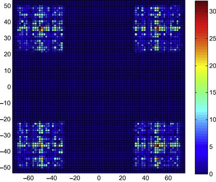
Let us now consider the case of the channel matrix:
We obtain Figures 4.3 and 4.4 respectively for the eye diagrams and the 2D-histograms. Clearly the channels are severe and close the eyes. Moreover, the pdf is obviously not separable, which attests to the non independency of the two components of ![]() .
.

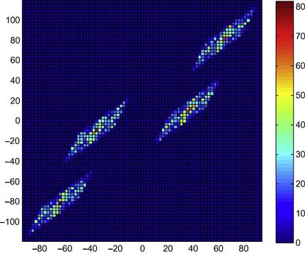
We run the JADE algorithm (see Sections 2.04.3.5 and 2.04.3.8) on the data (the observation duration is fixed to 1000 symbols): we obtain a ![]() matrix G such that, theoretically at least, GH should be diagonal. We form the data
matrix G such that, theoretically at least, GH should be diagonal. We form the data ![]() and plot Figures 4.5 and 4.6. The eyes have been opened and the joint pdf is hence separable. This is not a surprise since we have computed the resulting matrix GH:
and plot Figures 4.5 and 4.6. The eyes have been opened and the joint pdf is hence separable. This is not a surprise since we have computed the resulting matrix GH:
which is close to a diagonal matrix. We need to explain why BSS has been successfully achieved in this simple example and why it can also be achieved in much more difficult contexts.


2.04.1.3 Organisation of the paper
This chapter is organized as follows. In Section 2.04.2, we provide the model of the signals which are supposed to be linear modulations of symbols (Section 2.04.2.1). We discuss the statistics of the sampled versions of the transmitted sources in Section 2.04.2.2: in general, a sampled version is cyclo-stationary and we provide the basic tools and notation used along the paper. The model of the received data is specified in Section 2.04.2.3: (1) If the propagation channel between each transmitter and the receiver is a single path channel, the received signal is an instantaneous mixture of the transmitted signals; (2) if at least one of the propagation channel is a multipath channel, the mixture appears to be convolutive. Besides, we discuss the assumptions under which the received data are stationary. In general, however, the data are cyclo-stationary with unknown cyclic frequencies.
The case of instantaneous mixtures is addressed in Section 2.04.3. When the sources are independent and identically distributed (i.i.d.) (this case is discussed in Section 2.04.2.3), and that strong a priori information on the constellations are known, it is possible to provide algebraic solutions to the BSS problem, e.g., the Iterative Least Squares Projections (ILSP) algorithm or the Algebraic Constant Modulus Algorithms (ACMA): these methods are explained in Section 2.04.3.2. In Section 2.04.3.3, we consider the case of second-order methods (one of the advantages of these latter is that they are robust to the cyclo-stationarities, hence can be applied to general scenarios): the outlines of one of the most popular approach, the Second-Order Blind Identification (SOBI) algorithm, which consists in estimating the mixing matrix from the autocorrelation function of the received signal. This approach is conceptually simple, and the corresponding scheme allows one to identify the mixture and hence, to separate the source signals. That SOBI is rarely considered for BSS of digital communication signals is explained. The subsections that follow cope with BSS methods based on fourth-order cumulants. They are called “direct” BSS methods since they provide estimates of the sources with no prior estimation of the unknown channel matrix. For pedagogical and historical reasons, we firstly cope with the very particular case of stationary signals. One-by-one methods based are explained (Section 2.04.3.4) and are shown to be convergent; the associated deflation procedure is introduced and an improvement is presented. Global methods (also called joint separating methods) aim at separating jointly the K sources: they are depicted in Section 2.04.3.5; these approaches are based on the minimization of well chosen contrast functions over the set of ![]() unitary matrices: the famous Joint Approximate Diagonalization of Eigenmatrices (JADE) algorithm is presented, since it represents a touchstone in the domain of BSS. When the sources are cyclo-stationary, which is really the interesting point for the context of this paper, the preceding “stationary” methods (one-by-one and global) are again considered. The following problem is addressed: do the convergence result still hold when the algorithms are fed by cyclo-stationary data instead of stationary ones? Sufficient conditions are shown to assure the convergence: semi-analytical computations (Section 2.04.3.9) prove that the conditions in question hold true.
unitary matrices: the famous Joint Approximate Diagonalization of Eigenmatrices (JADE) algorithm is presented, since it represents a touchstone in the domain of BSS. When the sources are cyclo-stationary, which is really the interesting point for the context of this paper, the preceding “stationary” methods (one-by-one and global) are again considered. The following problem is addressed: do the convergence result still hold when the algorithms are fed by cyclo-stationary data instead of stationary ones? Sufficient conditions are shown to assure the convergence: semi-analytical computations (Section 2.04.3.9) prove that the conditions in question hold true.
In Sections 2.04.4 and 2.04.5, the case of convolutive mixtures is addressed. In certain particular scenarios, e.g., sparse channels, the gap between the instantaneous case and the convolutive one can be bridged quite directly (Section 2.04.4). More precisely, if the delays of the various multipaths are sufficiently spread out on the one hand and if, on the other hand, the number of antennas of the receiver is large enough, it is still possible to formulate the source separation problem as the separation of a certain instantaneous mixture. If these conditions do not hold, we face a real convolutive mixture, i.e., the received data are the output of a Multi-Input/Multi-Output (MIMO) unknown filter driven by jointly independent (cyclo-) stationary sources. Due to their historical and theoretical importance, we present algebraic methods (Section 2.04.5.1) when the data are stationary. Under this latter assumption, the identification of the unknown transfer function can be achieved using standard methods using the Moving Average (MA) or Auto-Regressive (AR) properties: see Section 2.04.5.2. The famous subspace method, introduced in Section 2.04.5.3, is based on second-order moments and can be used for general cyclo-stationary data; its inherent numerical problems are discussed. In Section 2.04.5.4, global direct methods are evoked (temporal domain and frequency domain) for stationary data. In Section 2.04.5.5, the case of one-to-one methods previously introduced in Section 2.04.3.4 is extended to the convolutive case and positive results for BSS are provided. The results are further extended for the cyclo-stationary case in Section 2.04.5.6 where convergence results are shown.
In Section 2.04.7, we discuss several points that have not been developed in the core of the paper. Further bibliographic entries are provided.
2.04.2 Signals
We have specified in the Introduction that the domain of source separation is not restricted to the context of telecommunication signals. In the following, however, most of the results apply specifically to digital telecommunication signals.
2.04.2.1 Source signals. Basic assumptions
We assume that K digital telecommunication devices simultaneously transmit information in the same band of frequencies. For ![]() , we denote by
, we denote by ![]() the complex envelope of the kth transmitted signal (“the kth source”). The subscript “a” in
the complex envelope of the kth transmitted signal (“the kth source”). The subscript “a” in ![]() underlines that the signal is “analog”. Throughout this contribution,
underlines that the signal is “analog”. Throughout this contribution, ![]() is supposed to stem from a linear modulation of a sequence of symbols. The model is hence:
is supposed to stem from a linear modulation of a sequence of symbols. The model is hence:
![]() (4.1)
(4.1)
In this latter equation, ![]() is a sequence of symbols belonging to a certain constellation. The function
is a sequence of symbols belonging to a certain constellation. The function ![]() is a shaping function and
is a shaping function and ![]() is the duration of a symbol
is the duration of a symbol ![]() . We denote by
. We denote by ![]() the carrier frequency associated with the kth source. Along this contribution, the following assumptions and notation are adopted.Assumptions on the source signals: For a given index k, the sequence
the carrier frequency associated with the kth source. Along this contribution, the following assumptions and notation are adopted.Assumptions on the source signals: For a given index k, the sequence ![]() is assumed to be independent and identically distributed (i.i.d.). We assume that it has zero mean
is assumed to be independent and identically distributed (i.i.d.). We assume that it has zero mean ![]() . With no restriction at all, the normalization
. With no restriction at all, the normalization ![]() holds. We also suppose that it is second-order complex-circular in the sense that
holds. We also suppose that it is second-order complex-circular in the sense that
![]() (4.2)
(4.2)
It is undoubtedly a restriction to impose the condition (4.2) especially in the telecommunication context of this paper; indeed, the BPSK modulation for instance does not verify (4.2). Some points on the extensions to general non circular mixtures are provided in Section 2.04.7.1.
The Kurtosis of the symbol ![]() , is defined as
, is defined as
![]()
where the fourth-order cumulant of a complex-valued random variable X is defined when it makes sense, as ![]() : see for instance [6]. Here, by the circularity Assumption 4.2, we have
: see for instance [6]. Here, by the circularity Assumption 4.2, we have
![]()
We assume that we have, for any index k:
![]() (4.3)
(4.3)
This inequality is given as an assumption; is has more the flavor of a result, since we do not know complex-circular constellations such that (4.3) is not satisfied.
We may now come to the key assumption: the sources ![]() are mutually independent.
are mutually independent.
Concerning the shaping filter, ![]() we suppose that
we suppose that ![]() is a square-root raised cosine with excess bandwidth (also called roll-off factor)
is a square-root raised cosine with excess bandwidth (also called roll-off factor) ![]() .
.
2.04.2.2 Cyclo-stationarity of a source
In this short paragraph, we drop the index of the source and ![]() refer to respectively
refer to respectively ![]() . Thanks to Eq. (4.1), it is quite obvious that
. Thanks to Eq. (4.1), it is quite obvious that ![]() and
and ![]() are similarly distributed since
are similarly distributed since ![]() is i.i.d. This simple reasoning applies to any vector
is i.i.d. This simple reasoning applies to any vector ![]() whose distribution equals this of
whose distribution equals this of ![]() . This shows that the process
. This shows that the process ![]() is cyclo-stationary in the strict sense with period T. In particular, its second and fourth-order moments evolve as T-periodic functions of the time. Let us focus on the second-order moments:
is cyclo-stationary in the strict sense with period T. In particular, its second and fourth-order moments evolve as T-periodic functions of the time. Let us focus on the second-order moments: ![]() is hence a periodic function with period T. We let its Fourier expansion be
is hence a periodic function with period T. We let its Fourier expansion be
![]() (4.4)
(4.4)
where ![]() is called “cyclo-correlation” of
is called “cyclo-correlation” of ![]() at cyclic frequency
at cyclic frequency ![]() and time lag
and time lag ![]() . We have the reverse formula:
. We have the reverse formula:
![]()
or
![]()
Generally, we may introduce the cyclo-correlation at any cyclic frequency ![]() :
:
![]()
In the case of ![]() given by Eq. (4.1),
given by Eq. (4.1), ![]() is identically zero for cyclic frequencies
is identically zero for cyclic frequencies ![]() that are not multiples of
that are not multiples of ![]() . In passing, we have the following symmetry:
. In passing, we have the following symmetry:
![]() (4.5)
(4.5)
Let us inspect a bit further a main specificity of linear modulations on the Fourier expansion of Eq. (4.4). In this respect, denote by ![]() the Fourier transform of the cyclo-correlation function
the Fourier transform of the cyclo-correlation function ![]() . We have, after elementary calculus (see [7,8]):
. We have, after elementary calculus (see [7,8]):
![]()
where ![]() is the Fourier transform of
is the Fourier transform of ![]() . This formula is visibly a generalization of the so-called Benett Equality (see [9]Section 4.4.1) that gives the power spectral density of
. This formula is visibly a generalization of the so-called Benett Equality (see [9]Section 4.4.1) that gives the power spectral density of ![]() : indeed, in the above equation, if one takes
: indeed, in the above equation, if one takes ![]() , we obtain
, we obtain ![]() which is the power spectral density. An important consequence was underlined in [8]:
which is the power spectral density. An important consequence was underlined in [8]:
Lemma 1
For any excess bandwidth factor![]() such that
such that![]() we have:
we have:
![]()
In other words, the cyclic frequencies of![]() given by Eq.(4.1)belong to the set
given by Eq.(4.1)belong to the set![]() .
.
Proof
The proof is obvious since the support of ![]() is
is ![]() with
with ![]() hence the supports of
hence the supports of ![]() and
and ![]() do not overlap except if
do not overlap except if ![]() .
. ![]()
We deduce from what precedes some consequences on the second-order statistics of a sampled version of a source. In this respect, we denote by ![]() any sampling period; the discrete-time signal associated with
any sampling period; the discrete-time signal associated with ![]() is hence
is hence ![]() for
for ![]() . Thanks to Lemma 1, the expansion (4.4) may be re-written as:
. Thanks to Lemma 1, the expansion (4.4) may be re-written as:
![]() (4.6)
(4.6)
where we let ![]() be
be ![]() . We distinguish between three cases:
. We distinguish between three cases:
1. If ![]() is a integer, the three terms of the r.h.s. of (4.6) all aggregate in a single term, making the function
is a integer, the three terms of the r.h.s. of (4.6) all aggregate in a single term, making the function ![]() not depend on the time index n. This is not surprising since the condition
not depend on the time index n. This is not surprising since the condition ![]() where p is a non-null integer corresponds to a strict-sense stationary signal (see the polyphase decomposition in [10]). In particular, if
where p is a non-null integer corresponds to a strict-sense stationary signal (see the polyphase decomposition in [10]). In particular, if ![]() , we have:
, we have:
![]() (4.7)
(4.7)
where ![]() . In the following, we will not study the case
. In the following, we will not study the case ![]() with
with ![]() .
.
2. If ![]() modulo
modulo ![]() : unless
: unless ![]() is rational, it cannot be said that, as a function of
is rational, it cannot be said that, as a function of ![]() is periodic: it is called an almost periodic function [11] and
is periodic: it is called an almost periodic function [11] and ![]() is hence called almost periodically correlated, having
is hence called almost periodically correlated, having ![]() as cyclic-frequencies. We introduce
as cyclic-frequencies. We introduce
![]() (4.8)
(4.8)
where the operator ![]() is the time-averaging one, i.e., for a complex-valued (deterministic) series
is the time-averaging one, i.e., for a complex-valued (deterministic) series ![]()
when the limit makes sense. As the three cyclic-frequencies in the expansion (4.6) are distinct modulo 1 then we obtain
![]()
which reminds us of the Shannon sampling theorem.
3. If ![]() it turns out that, similarly to the previous case, the discrete-time source is cyclo-stationary, having
it turns out that, similarly to the previous case, the discrete-time source is cyclo-stationary, having ![]() as cyclic- frequencies. Moreover
as cyclic- frequencies. Moreover ![]() and
and ![]() .
.
2.04.2.3 Received signals
The receiver is equipped with M antennas, the number of antennas being as big as the number of sources, i.e., ![]() (see section 2.04.2.3.2). We denote by
(see section 2.04.2.3.2). We denote by

the complex envelope of the received ![]() vector computed at a frequency of demodulation denoted by
vector computed at a frequency of demodulation denoted by ![]() . We consider that
. We consider that ![]() obeys the linear model
obeys the linear model

where ![]() is the contribution of the kth source to the observation. We further assume that
is the contribution of the kth source to the observation. We further assume that ![]() stems from delayed/attenuated versions of
stems from delayed/attenuated versions of ![]() . In this respect, we may write
. In this respect, we may write ![]() , the component of
, the component of ![]() associated with the mth sensor, as:
associated with the mth sensor, as:
 (4.9)
(4.9)
where the index ![]() represents the path index,
represents the path index, ![]() the number of paths associated with the source no
the number of paths associated with the source no ![]() an attenuation factor and
an attenuation factor and ![]() the delay of the propagation along the path no
the delay of the propagation along the path no ![]() between the source no k and the sensor no m. In this latter equation,
between the source no k and the sensor no m. In this latter equation, ![]() is the complex envelope of the modulated signal
is the complex envelope of the modulated signal ![]() at the demodulation frequency, i.e.,
at the demodulation frequency, i.e., ![]() .
.
2.04.2.3.1 Models of the sampled data
We distinguish between two cases:
1. Instantaneous mixture: This scenario holds when the signal ![]() evolves in a linear space of dimension 1, that is when the components
evolves in a linear space of dimension 1, that is when the components ![]() in (4.9) do not depend neither on
in (4.9) do not depend neither on ![]() nor on m. This holds when there exists
nor on m. This holds when there exists ![]() such that
such that ![]() for all indices
for all indices ![]() . This happens, for instance, when there is a single path (
. This happens, for instance, when there is a single path (![]() ) and the transmitted signal is narrow-band (
) and the transmitted signal is narrow-band (![]() ). In this case we have
). In this case we have

More compactly, this gives
![]()
where ![]() is a
is a ![]() mixing matrix, and
mixing matrix, and
![]() (4.10)
(4.10)
If ![]() is the sampling period of the receiver, it is supposed that all the components of the data are low-pass filtered in the sampling band (the matched-filter cannot be considered since the shaping filters are not supposed to be known to the receiver). Finally, the (noiseless model) of the data is
is the sampling period of the receiver, it is supposed that all the components of the data are low-pass filtered in the sampling band (the matched-filter cannot be considered since the shaping filters are not supposed to be known to the receiver). Finally, the (noiseless model) of the data is
![]() (4.11)
(4.11)
where
![]() (4.12)
(4.12)
Generally speaking, any of the components of the source vector ![]() is cyclo-stationary (see Section 2.04.2.2) hence the model given by (4.11) is a cyclo-stationary one. For simplification, let us suppose in the following that
is cyclo-stationary (see Section 2.04.2.2) hence the model given by (4.11) is a cyclo-stationary one. For simplification, let us suppose in the following that ![]() for all the indices k (this point is discussed in Section 2.04.7). As the original theory of BSS assumed stationary data, we inspect under which conditions the above model can be stationary. A necessary and sufficient condition is that all the components of
for all the indices k (this point is discussed in Section 2.04.7). As the original theory of BSS assumed stationary data, we inspect under which conditions the above model can be stationary. A necessary and sufficient condition is that all the components of ![]() be stationary. As discussed previously, this can happen when all the symbol periods are equal to, say, T and if the sampling period
be stationary. As discussed previously, this can happen when all the symbol periods are equal to, say, T and if the sampling period ![]() . Under these conditions, we even have:
. Under these conditions, we even have:
![]()
where we have set for any delay ![]()
![]() (4.13)
(4.13)
The stationary model can be written as:
![]() (4.14)
(4.14)
where we have set
 (4.15)
(note: the notation might be confusing since ![]() was already defined in (4.12): in the following sections, the context is always specified which prevents the confusion) In the literature, it is sometimes required that the sources be i.i.d. In the context of this paper, this i.i.d. condition is fulfilled when the filters
was already defined in (4.12): in the following sections, the context is always specified which prevents the confusion) In the literature, it is sometimes required that the sources be i.i.d. In the context of this paper, this i.i.d. condition is fulfilled when the filters ![]() all have the form of a constant times a delay: in short, this happens when (1) all the transmitted symbols are synchronized (2) the receiver runs a matched filter (square-root Nyquist), and (3) the symbol synchronization is performed at the receiver. In this case we have:
all have the form of a constant times a delay: in short, this happens when (1) all the transmitted symbols are synchronized (2) the receiver runs a matched filter (square-root Nyquist), and (3) the symbol synchronization is performed at the receiver. In this case we have:
 (4.16)
The reader may find this set of condition very restrictive in real scenarios. It is indeed; however, the developments of BSS are based on the stationary assumption. Moreover, many interesting methods exploit the i.i.d. condition.
2. Convolutive mixture: This is the general case when multi-paths affect the propagation. We provide the discrete-time version of Eq. (4.9). Let us begin by the general case. In this respect, we assume that the sampling period ![]() verifies the Shannon sampling condition, i.e.,
verifies the Shannon sampling condition, i.e.,
![]()
This is a non-restrictive condition whatever the scenario: a crude prior spectral analysis of the data is simply needed. Provided this condition, the discrete-time signal ![]() , for any indices
, for any indices ![]() , is a filtered version of
, is a filtered version of ![]() . It is hence easy to deduce that the sampled data
. It is hence easy to deduce that the sampled data ![]() follows the equation:
follows the equation:
![]() (4.17)
(4.17)
where ![]() is a vector of mutually independent sources and
is a vector of mutually independent sources and ![]() is certain the
is certain the ![]() transfer function whose kth column is the digital channel between the kth source and the receiver: it depends on the parameters
transfer function whose kth column is the digital channel between the kth source and the receiver: it depends on the parameters ![]() . The above general model is, in general, cyclo-stationary. For simplification, we assume ion the following that
. The above general model is, in general, cyclo-stationary. For simplification, we assume ion the following that ![]() for all indices k. Similarly to the case of instantaneous mixtures, it is instructive to find conditions under which the data are stationary. This occurs when the symbol periods
for all indices k. Similarly to the case of instantaneous mixtures, it is instructive to find conditions under which the data are stationary. This occurs when the symbol periods ![]() all coincide with a certain T, and when the sampling period
all coincide with a certain T, and when the sampling period ![]() equals T. Under all these conditions,
equals T. Under all these conditions, ![]() , the contribution of the kth source to the mixture, can be written as
, the contribution of the kth source to the mixture, can be written as

![]() (4.18)
(4.18)
where ![]() and
and ![]() is a certain
is a certain ![]() unknown filter matrix. This shows that
unknown filter matrix. This shows that ![]() depends on the shaping filters, the steering vectors associated with the paths and their corresponding delays.
depends on the shaping filters, the steering vectors associated with the paths and their corresponding delays.
2.04.2.3.2 Assumptions on the channels
In this paper, we consider over-determined mixtures, that is: mixtures such that the number of sensors exceeds the number of sources (![]() ). This condition is necessary in order to retrieve the vector
). This condition is necessary in order to retrieve the vector ![]() —see model (4.11) (respectively (4.17) )—from the data
—see model (4.11) (respectively (4.17) )—from the data ![]() by means of a
by means of a ![]() constant matrix (respectively a
constant matrix (respectively a ![]() filter). This has to be specified.
filter). This has to be specified.
For instantaneous mixtures, the following condition holds:
![]() (4.19)
(4.19)
Under this assumption, there exist ![]() matrices
matrices ![]() such that
such that ![]() .
.
For convolutive mixtures, it is conventional to assume that the components of ![]() are polynomials in
are polynomials in ![]() (this is an approximation that is justified since the shaping filters
(this is an approximation that is justified since the shaping filters ![]() are rapidly vanishing when
are rapidly vanishing when ![]() ). We further assume that
). We further assume that
![]() (4.20)
(4.20)
Under this condition, there exist polynomial matrices ![]() such that
such that ![]() : see for instance [12,13]. The same kind of assumption holds in the stationary case—see the model (4.18): namely,
: see for instance [12,13]. The same kind of assumption holds in the stationary case—see the model (4.18): namely,
![]() (4.21)
(4.21)
At this level, we would like to point out a curiosity. In this respect, we assume further that the excess bandwidth factors of one source—say the first one—equals zero. As the choice ![]() satisfies the Shannon sampling condition, we may write
satisfies the Shannon sampling condition, we may write ![]() where
where
![]()
As ![]() , the first column
, the first column ![]() of
of ![]() can be factored as
can be factored as ![]() . In particular, after the standard FIR approximations, it yields that the condition given in (4.21) is not fulfilled.
. In particular, after the standard FIR approximations, it yields that the condition given in (4.21) is not fulfilled.
2.04.3 Instantaneous mixtures
The model of the data ![]() is given by (4.11). The mixing matrix
is given by (4.11). The mixing matrix ![]() is unknown. BSS can be achieved either by estimating
is unknown. BSS can be achieved either by estimating ![]() —this is the point of Section 2.04.3.3—or by computing directly estimates of the sources (up to indeterminacies).
—this is the point of Section 2.04.3.3—or by computing directly estimates of the sources (up to indeterminacies).
2.04.3.1 Indeterminacies
It is always possible to consider that the sources have equal and normalized power. Indeed, as ![]() where
where ![]() is the square-root of the power of the first source, we suggest to scale the first column of
is the square-root of the power of the first source, we suggest to scale the first column of ![]() by
by ![]() . Repeating this process for all the sources, we have constructed a new matrix
. Repeating this process for all the sources, we have constructed a new matrix ![]() . Eventually denoting
. Eventually denoting ![]() , we obviously show that the data alternatively writes
, we obviously show that the data alternatively writes
![]()
Though apparently innocent, this remark gives precious a priori indications. First of all, it says that the model (4.22) is not uniquely defined. As a consequence, it is always possible to consider, without restricting the model, that the sources have equal power equal to one—this precisely corresponds to the above defined ![]() ; specifically, we will assume in the following that
; specifically, we will assume in the following that
![]() (4.22)
(4.22)
This shows it is beyond a reasonable expectation to retrieve the sources with no scaling ambiguities. Similarly, if ![]() is a permutation matrix,
is a permutation matrix, ![]() , underlining the non-unicity of the model.
, underlining the non-unicity of the model.
With no further assumptions on the sources, the ultimate result that can be achieved is: retrieve the sources up to unknown complex scaling factors (scaling and phase ambiguities) and a permutation.
2.04.3.2 Algebraic methods (i.i.d. scenario)
The model of the data is given by (4.16). We may collect the N available data in a ![]() matrix
matrix ![]() , we have:
, we have: ![]() where
where ![]() . As any entry of
. As any entry of ![]() corresponds to a symbol, associated specificities (e.g., finite alphabet constellations or modulus one symbols) are a priori relations the receiver can make use of. As far as the identifiability is concerned, it is proven in [14] (Lemma 1) that the above factorization is essentially unique for modulus one symbols, at least if the number of snapshots N verifies
corresponds to a symbol, associated specificities (e.g., finite alphabet constellations or modulus one symbols) are a priori relations the receiver can make use of. As far as the identifiability is concerned, it is proven in [14] (Lemma 1) that the above factorization is essentially unique for modulus one symbols, at least if the number of snapshots N verifies ![]() (which is the case in practical contexts). By essentially unique, we mean that the rows of
(which is the case in practical contexts). By essentially unique, we mean that the rows of ![]() may be permuted and/or multiplied by modulus one constants.
may be permuted and/or multiplied by modulus one constants.
Talwar et al. [15,16] propose iterative algorithms that assume known the alphabets of the symbols. Call ![]() an estimate of
an estimate of ![]() at the iteration no
at the iteration no ![]() . The Iterative Least Square with Projection (ILSP) is:
. The Iterative Least Square with Projection (ILSP) is:
1. Take any full rank ![]() for iteration
for iteration ![]()
• ![]() where
where ![]() denotes the pseudo-inverse.
denotes the pseudo-inverse.
• ![]() projection of each component of
projection of each component of ![]() on the corresponding alphabet.
on the corresponding alphabet.
Similar projection-based algorithms that rather take into account the constant modulus property of the entries of ![]() have been considered [17,18]: similarly to the IMSP algorithm, no results on the convergence can be given (how many samples are required? are there local minima the algorithm could be trapped in?). Van der Veen et al. [14] proposes a non-iterative algorithm, called the Algebraic CMA (ACMA): the ACMA provides exactly “the” solution (up to the above mentioned ambiguities) of the factorization of
have been considered [17,18]: similarly to the IMSP algorithm, no results on the convergence can be given (how many samples are required? are there local minima the algorithm could be trapped in?). Van der Veen et al. [14] proposes a non-iterative algorithm, called the Algebraic CMA (ACMA): the ACMA provides exactly “the” solution (up to the above mentioned ambiguities) of the factorization of ![]() —at least if the number of data N exceeds
—at least if the number of data N exceeds ![]() . It is based on a joint diagonalization of a pencil of K matrices.
. It is based on a joint diagonalization of a pencil of K matrices.
Certain BSS methods for convolutive mixtures need, as a final step, to run such algorithms (see e.g., Section 2.04.5.1).
2.04.3.3 Second-order based identification (general cyclo-stationary case)
In this section, we address the “indirect” BSS; by this terminology, we mean that the BSS is achieved in two steps. The first step consists in estimating the unknown mixing matrix H by, say, ![]() . In a second step, the proper separation is carried out. If
. In a second step, the proper separation is carried out. If ![]() is an accurate estimate, then
is an accurate estimate, then ![]() is the natural estimate of the source vector. In general, however, noise is present (estimation noise and additive noise in the observed signals) and other strategies have to be considered: this aspect is not addressed in this paper.
is the natural estimate of the source vector. In general, however, noise is present (estimation noise and additive noise in the observed signals) and other strategies have to be considered: this aspect is not addressed in this paper.
The first point to be addressed in this section is the pre-whitening of the data. We suppose that ![]() (notice: in the non-square case, a principal component analysis is processed). In this respect, we consider the auto-correlation matrix of the data
(notice: in the non-square case, a principal component analysis is processed). In this respect, we consider the auto-correlation matrix of the data ![]() can be written (we recall that the sources are assumed to have equal normalized powers as discussed previously):
can be written (we recall that the sources are assumed to have equal normalized powers as discussed previously):
![]()
Since ![]() is full rank, the above matrix is positive definite and we form the new data
is full rank, the above matrix is positive definite and we form the new data
![]()
We have:
![]()
where ![]() is a unitary matrix.
is a unitary matrix.
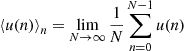
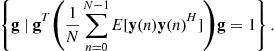
The second point concerns the estimation of the unitary matrix U. The data ![]() is cyclo-stationary. As the cyclic-frequencies are not always directly accessible, the identification of the unknown mixing matrix U is done by solely considering the statistics
is cyclo-stationary. As the cyclic-frequencies are not always directly accessible, the identification of the unknown mixing matrix U is done by solely considering the statistics
![]()
which can be expressed as
![]()
This says that the normal matrix ![]() , for any index
, for any index ![]() , is diagonalized in the orthonormal basis formed by the columns of U. For
, is diagonalized in the orthonormal basis formed by the columns of U. For ![]() , this gives
, this gives ![]() and this is clearly not sufficient to identify U! On the contrary, consider that the spectra of the sources
and this is clearly not sufficient to identify U! On the contrary, consider that the spectra of the sources ![]() are all different at least for a frequency
are all different at least for a frequency ![]() . For any unitary matrix
. For any unitary matrix ![]() , the matrix
, the matrix ![]() is diagonal for every indices
is diagonal for every indices ![]() if and only if the columns of
if and only if the columns of ![]() equal these of U up to a modulus one factor and a permutation. This remark was done in [19] and an algorithm (SOBI) was deduced based on a joint diagonalization technique [20].
equal these of U up to a modulus one factor and a permutation. This remark was done in [19] and an algorithm (SOBI) was deduced based on a joint diagonalization technique [20].
The reader has noticed the suboptimality of the above method when the mixture is cyclo-stationary. The exploited statistics are only the ![]() for certain indices
for certain indices ![]() . In [21], it is suggested to take advantage of the cyclic-statistics of the mixture. In this respect, notice that for any
. In [21], it is suggested to take advantage of the cyclic-statistics of the mixture. In this respect, notice that for any ![]() cyclic frequency of the mixture, we have
cyclic frequency of the mixture, we have
![]()
hence these “new” statistics could be added in the pencil of matrices to be jointly diagonalized. This theoretical appeal is attenuated by the fact that the non null-components of ![]() are numerically inconsistent.
are numerically inconsistent.
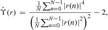
At this level, we should emphasize that the statistics ![]() for any
for any ![]() (zero or not) are not accessible to the receiver and should be replaced by the empirical estimate denoted by
(zero or not) are not accessible to the receiver and should be replaced by the empirical estimate denoted by ![]() and defined for
and defined for ![]() as
as
 (4.23)
where N is the number of snapshots. This estimate is a consistent estimate of the matrix ![]() . In an ideal scenario where the model
. In an ideal scenario where the model ![]() holds true, it is remarkable that
holds true, it is remarkable that ![]() and the joint diagonalization of the estimated statistics should provide the exact mixing matrix: the algorithm is called deterministic. In a realistic context, however, the data are perturbed by an additive noise term: in this case, the above factorization does not hold true anymore and the joint diagonalization is an approximate joint diagonalization.
and the joint diagonalization of the estimated statistics should provide the exact mixing matrix: the algorithm is called deterministic. In a realistic context, however, the data are perturbed by an additive noise term: in this case, the above factorization does not hold true anymore and the joint diagonalization is an approximate joint diagonalization.
In practice, despite its attractivity, SOBI is seldom used to achieve BSS of digital communication data. Indeed, the condition that there are no two sources whose spectra are identical (up to a multiplicative constant) does not make sense most of the time. Indeed, the transmitted symbols are generally white sequences whose shaping functions are close from to one another. As the spectra are numerically similar, the joint diagonalization approach is bound to suffer from numerical problems.
2.04.3.4 Iterative BSS (stationary case)
As was specified, the stationary scenario assumes that for all indices ![]() , i.e., all the baud-rates are equal, and
, i.e., all the baud-rates are equal, and ![]() . Under these very specific circumstances, the model (4.14) involves a source vector
. Under these very specific circumstances, the model (4.14) involves a source vector ![]() whose components are stationary and mutually independent. We insist on the fact that the components of the source vector are not the i.i.d. symbol sequences but linear processes generated by these symbol sequences as indicated by Eq. (4.15). BSS aims at estimating the sources, not the symbol sequences. Hence, BSS may be seen as a preliminary step before the estimation of the symbols.
whose components are stationary and mutually independent. We insist on the fact that the components of the source vector are not the i.i.d. symbol sequences but linear processes generated by these symbol sequences as indicated by Eq. (4.15). BSS aims at estimating the sources, not the symbol sequences. Hence, BSS may be seen as a preliminary step before the estimation of the symbols.
Contrary to other methods, no pre-processing of the data is necessary (PCA, pre-whitening).
In this section, we firstly design methods able to recover one of the sources (or a scaled version). In a second step, we present the so-called deflation that allows one to run the extraction of another source from a deflated mixture where the contribution of the first estimated source has been removed. The convergence is established: after K such steps, the K sources are expected to be estimated. Convergence properties are discussed.
2.04.3.4.1 Estimation of one source: theoretical considerations
Thanks to the mixing matrix ![]() having full-rank—see condition (4.19)—we know that, for any source index k, there exist column vectors
having full-rank—see condition (4.19)—we know that, for any source index k, there exist column vectors ![]() such that
such that
![]()
Denoting ![]() , we may call this new signal as the reconstructed source since it involves only one source. This new signal is obtained after a so-called spatial filtering of the data. Of course, it is not possible to compute
, we may call this new signal as the reconstructed source since it involves only one source. This new signal is obtained after a so-called spatial filtering of the data. Of course, it is not possible to compute ![]() since H is not accessible. A possible approach hence consists in adapting a spatial filter g that makes
since H is not accessible. A possible approach hence consists in adapting a spatial filter g that makes
![]() (4.24)
(4.24)
resemble one of the sources. This will be done by considering particular statistics of the signal ![]() . We may write this signal under this form
. We may write this signal under this form
 (4.25)
where the taps ![]() are the components of the vector
are the components of the vector
![]() (4.26)
(4.26)
The term ![]() in
in ![]() represents the contribution of the kth source to the reconstructed signal
represents the contribution of the kth source to the reconstructed signal ![]() . As may be easily understood, we aim at finding a “good”
. As may be easily understood, we aim at finding a “good” ![]() , i.e., such that f is a vector having a single non-null component.
, i.e., such that f is a vector having a single non-null component.
Definition 2
A vector ![]() is said to be separating if all its components are null except one.
is said to be separating if all its components are null except one.
Evidently, the signal ![]() involves a single source if and only if the composite vector
involves a single source if and only if the composite vector ![]() is separating.
is separating.
We may inspect higher-order statistics and particularly the fourth-order ones. It has been proposed to consider the fourth-order cumulant (see Section 2.04.3.6 for theoretical justifications):
![]()
In this respect, we may introduce the following function, called normalized (fourth-order) cumulant:
![]() (4.27)
(4.27)
Thanks to the definition of the cumulants, we have: ![]() . Now, the circularity assumption of the symbol sequences (4.2) implies the circularity of the sources, hence
. Now, the circularity assumption of the symbol sequences (4.2) implies the circularity of the sources, hence
![]()
We re-express ![]() as a function of the moments of
as a function of the moments of ![]() :
:
 (4.28)
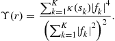
Proposition 3
As, by assumption, the Kurtosis of the sources,![]() , are strictly negative, the function
, are strictly negative, the function![]() achieves its minimum at a separating vector. Moreover, the separating vector in question has its single non-null element located at an index
achieves its minimum at a separating vector. Moreover, the separating vector in question has its single non-null element located at an index![]() such that
such that![]() .
.
Proof
On the one hand, the mixture ![]() is a linear mixture of independent random variables. The multi-linearity of the cumulants [6] gives:
is a linear mixture of independent random variables. The multi-linearity of the cumulants [6] gives:

After noticing that ![]() we arrive at the expansion:
we arrive at the expansion:
 (4.29)
On the other hand, ![]() is a linear process generated by the i.i.d. symbol sequence
is a linear process generated by the i.i.d. symbol sequence ![]() : see Eq. (4.7). As was supposed (or noticed) in the Introduction,
: see Eq. (4.7). As was supposed (or noticed) in the Introduction, ![]() hence
hence
![]()
for any index k. The sources are sometimes referred to as platykurtic sources. Denote by ![]() . Thanks to the above result,
. Thanks to the above result, ![]() . Hence
. Hence ![]() . Besides, we recall that
. Besides, we recall that ![]() with equality if and only if the coefficients
with equality if and only if the coefficients ![]() are all null except one, i.e., if and only if the vector
are all null except one, i.e., if and only if the vector ![]() is separating.
is separating.
We insist on the fact that the assumption that one of the ![]() is strictly negative is fundamental. Imagine on the contrary that, for all the indices
is strictly negative is fundamental. Imagine on the contrary that, for all the indices ![]() . Then
. Then ![]() . As
. As
with equality iff all the ![]() are equal, this implies that the argument minima of
are equal, this implies that the argument minima of ![]() are not separating (on the contrary, the coefficients
are not separating (on the contrary, the coefficients ![]() equally weigh the sources).
equally weigh the sources). ![]()
As a remark, it is instructive, though superfluous in this paper since the digital communication symbols have negative Kurtosis, to address the optimization of ![]() for general distributions of the
for general distributions of the ![]() : the reader may find the details in [5].
: the reader may find the details in [5].
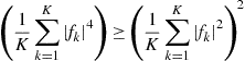
One may inspect the minimum minimorum of ![]() over all the possible constellations. The Jensen inequality (see [22] p. 80) gives:
over all the possible constellations. The Jensen inequality (see [22] p. 80) gives: ![]() for a convex mapping
for a convex mapping ![]() ; the equality is achieved when
; the equality is achieved when ![]() . Taking
. Taking ![]() , we obtain
, we obtain
![]()
and the equality is achieved when ![]() has unit modulus. Of course, this can only happen if one of the sources has a modulus equal to one or, there exists an index k such that
has unit modulus. Of course, this can only happen if one of the sources has a modulus equal to one or, there exists an index k such that ![]() . This does not happen in general, but this remark shows that the minimization of
. This does not happen in general, but this remark shows that the minimization of ![]() tends to make
tends to make ![]() resemble as much as possible a constant modulus sequence. We inspect this point a bit further. A way to measure the distance of
resemble as much as possible a constant modulus sequence. We inspect this point a bit further. A way to measure the distance of ![]() to the modulus one is simply to consider
to the modulus one is simply to consider
![]() (4.30)
(4.30)
This function was originally considered for deconvolution problems [23,24] and then for source separation problems ([25–27] for instance).
We may bridge the gap between ![]() and
and ![]() :
:
Proposition 4
Define![]() and
and![]() . The minimization of
. The minimization of![]() is linked to the minimization of
is linked to the minimization of![]() in the sense that:
in the sense that:
![]()
iffachieves to minimize![]() then
then![]()
![]() is a minimizer of
is a minimizer of![]() . Conversely, if
. Conversely, if![]() achieves to minimize
achieves to minimize![]() , then
, then![]() minimizes
minimizes![]() for any
for any![]() .
.
Proof
For any f, we have: ![]() . Thanks to the expression of
. Thanks to the expression of ![]() in (4.28), it is always true that:
in (4.28), it is always true that: ![]() . We hence have:
. We hence have:
![]()
We set ![]() . The second-order polynomial
. The second-order polynomial ![]() has minimal value
has minimal value ![]() for
for ![]() . We deduce the inequality:
. We deduce the inequality: ![]() . If
. If ![]() reaches the infimum of
reaches the infimum of ![]() then, evidently, the choice
then, evidently, the choice ![]() makes
makes ![]() . Hence
. Hence ![]() is the minimum of
is the minimum of ![]() . Conversely, for any
. Conversely, for any ![]() , by definition, we have:
, by definition, we have: ![]() . In this inequality, substitute
. In this inequality, substitute ![]() for any positive
for any positive ![]() . We have:
. We have:
![]()
This is in particular true for ![]() hence showing that
hence showing that ![]() or
or
![]()
The case of equality in the latter equation occurs when ![]() is any non-null scaled version of a minimizer of
is any non-null scaled version of a minimizer of ![]()
![]()
As is explained in the next section, the search of a global minimum of ![]() or
or ![]() is done according to a gradient method. It is well known that such an algorithm may be stuck in a local minimum of the function to be minimized. We have the result (see [5], Lemma 1):
is done according to a gradient method. It is well known that such an algorithm may be stuck in a local minimum of the function to be minimized. We have the result (see [5], Lemma 1):
Lemma 5
Fix K real constants![]() . The local minima of the function
. The local minima of the function![]() over the unit sphere
over the unit sphere![]() are the separating vectors (of unit norm).
are the separating vectors (of unit norm).
Thanks to the expansion (4.29), and the fact that for all the sources ![]() , the local minima of
, the local minima of ![]() over the unit sphere are the separating vectors (of unit norm). After simple topological considerations, it can even be deduced that:
over the unit sphere are the separating vectors (of unit norm). After simple topological considerations, it can even be deduced that:
Proposition 6
Any local minimum of![]() is separating.
is separating.
As far as the function ![]() is concerned, we have:
is concerned, we have:
Proposition 7
Any local minimum of![]() is separating.
is separating.
Proof
We consider the arguments given in [28]. The idea consists in writing ![]() in its polar form
in its polar form ![]() where
where ![]() and
and ![]() . After setting
. After setting ![]() the normalized version of
the normalized version of ![]() , we have:
, we have: ![]() . Write this function
. Write this function ![]() . Necessarily, for a stationary point of
. Necessarily, for a stationary point of ![]() the derivative of
the derivative of ![]() w.r.t.
w.r.t. ![]() is zero. This gives:
is zero. This gives: ![]() or
or ![]() . The case
. The case ![]() can be shown to correspond to a local maximum [26]. This says that a local minimum of
can be shown to correspond to a local maximum [26]. This says that a local minimum of ![]() is a local minimum of
is a local minimum of ![]() . Now, this latter function is:
. Now, this latter function is:
![]()
We deduce that such a local minimum is also a local minimum of ![]() on the unit sphere. Thanks to Lemma 5 we deduce that the local minimum in question is separating.
on the unit sphere. Thanks to Lemma 5 we deduce that the local minimum in question is separating. ![]()
2.04.3.4.2 Estimation of one source: practical aspects
Basic algorithms: Two problems arise when one focuses on the implementation of the results presented so forth: the first one concerns the estimation of the cost functions ![]() or
or ![]() , the second one is to choose a method able to find the argument minima of these estimated functions.
, the second one is to choose a method able to find the argument minima of these estimated functions.
The two functions we have considered involve second and fourth-order moments of the signal ![]() . As the number of available data is finite—say, we observe
. As the number of available data is finite—say, we observe ![]() for
for ![]() —it is not possible to compute any of the moments of
—it is not possible to compute any of the moments of ![]() . However, a version of the law of large numbers allows one to consider estimates of the moments:
. However, a version of the law of large numbers allows one to consider estimates of the moments:
Lemma 8
For![]() , we have, with probability one:
, we have, with probability one:

We are in position to estimate both functions ![]() and
and ![]() respectively by
respectively by
 (4.31)
 (4.32)
Indeed, we have the result:
Proposition 9
![]() and
and![]() with probability one.
with probability one.
The functions ![]() and
and ![]() to be minimized are non-convex, and the associated machinery cannot be considered. The functions, however, are regular w.r.t. the parameter
to be minimized are non-convex, and the associated machinery cannot be considered. The functions, however, are regular w.r.t. the parameter ![]() . Hence, we choose to seek the argument minima by means of a gradient method. For instance, consider the minimization of
. Hence, we choose to seek the argument minima by means of a gradient method. For instance, consider the minimization of ![]() . The notation for the gradient of
. The notation for the gradient of ![]() calculated at the point
calculated at the point ![]() being
being ![]() , the gradient algorithm, for a fixed
, the gradient algorithm, for a fixed ![]() , can be written as:
, can be written as:
1. choose an initial vector ![]() and compute
and compute ![]() for all the available data;
for all the available data;
2. at the mth step: compute ![]() and the associated updated signal
and the associated updated signal ![]() ;
;
The same algorithm could be written for the minimization of ![]() . However, the fact this latter function is homogeneous may involve numerical problems (the vector
. However, the fact this latter function is homogeneous may involve numerical problems (the vector ![]() is not bounded). This is why the projected gradient algorithm is prefered: it consists in normalizing at each iteration of the algorithm the updated signal
is not bounded). This is why the projected gradient algorithm is prefered: it consists in normalizing at each iteration of the algorithm the updated signal ![]() , i.e., projecting the current parameter
, i.e., projecting the current parameter ![]() on the set
on the set
Whatever the considered cost function, the parameter ![]() controls the performance. The next section faces the problem of choosing
controls the performance. The next section faces the problem of choosing ![]() .Refinement: choosing a locally optimal
.Refinement: choosing a locally optimal ![]() . For simplicity, the minimization of
. For simplicity, the minimization of ![]() is addressed. The same idea may be considered for the minimization of
is addressed. The same idea may be considered for the minimization of ![]() by means of the projected gradient. In order to boost the speed of convergence, it has been proposed to change
by means of the projected gradient. In order to boost the speed of convergence, it has been proposed to change ![]() at each step of the algorithm: the parameter
at each step of the algorithm: the parameter ![]() is chosen such that the value of the function evaluated at the point
is chosen such that the value of the function evaluated at the point ![]() is minimum. It is easily seen that the function
is minimum. It is easily seen that the function ![]() is a polynomial of degree four. The minimum is hence easily (numerically) computed.Robustness of the algorithms to the presence of local minima: It is well-known that such a gradient algorithm may be trapped in a local minimum: this, in general, is a clear limitation to the use of such an algorithm. Of course, it is not possible to say much on the local minima of the estimated functions
is a polynomial of degree four. The minimum is hence easily (numerically) computed.Robustness of the algorithms to the presence of local minima: It is well-known that such a gradient algorithm may be trapped in a local minimum: this, in general, is a clear limitation to the use of such an algorithm. Of course, it is not possible to say much on the local minima of the estimated functions ![]() and
and ![]() . However, Propositions 6 and 7 indicate that, asymptotically, if the algorithms are trapped in a local minimum, this does not impact the performance since this local minimum is precisely separating. This remark certainly explains why the algorithms show very good performance.
. However, Propositions 6 and 7 indicate that, asymptotically, if the algorithms are trapped in a local minimum, this does not impact the performance since this local minimum is precisely separating. This remark certainly explains why the algorithms show very good performance.
2.04.3.4.3 The deflation step
The algorithms depicted above provide a way to retrieve one of the sources. Of course, we aim at estimating all the sources. An idea hence consists in running again the previous algorithm. However, it is not possible to guarantee that the second extracted source is not the first extracted one. In the literature, three methods have been presented that overcome this major problem.
In the first one [29] it is proposed to penalize the cost function ![]() or
or ![]() by adding to them a positive term that gives a measure of decorrelation between the current signal
by adding to them a positive term that gives a measure of decorrelation between the current signal ![]() and the previously extracted source. It is simple to show that, indeed, the global minimum is achieved if and only if the
and the previously extracted source. It is simple to show that, indeed, the global minimum is achieved if and only if the ![]() is an other source. However, this approach has been noticed to show poor performance. The reason is that the extended cost function, contrary to the original, has many local minima that do not correspond to separating solutions. The algorithms is known to be trapped in such local minima and, in this case, the provided solution is not an estimate of one of the remaining sources.
is an other source. However, this approach has been noticed to show poor performance. The reason is that the extended cost function, contrary to the original, has many local minima that do not correspond to separating solutions. The algorithms is known to be trapped in such local minima and, in this case, the provided solution is not an estimate of one of the remaining sources.
The second one is algebraic: the idea is to estimate the subspace associated with the first estimated source and to run the minimization of ![]() or
or ![]() on the orthogonal complement of the subspace in question: see [5].
on the orthogonal complement of the subspace in question: see [5].
The third is the most popular for source separation [30,31]: it consists in deflating the mixture by subtracting an estimation of the contribution of the extracted source and then to redo the minimization of ![]() or
or ![]() . Ideally, the “new” mixture should not involve the source that has been extracted and the minimization hence allows one to estimate another source. We provide some details.
. Ideally, the “new” mixture should not involve the source that has been extracted and the minimization hence allows one to estimate another source. We provide some details.
Thanks to the previous results, we may suppose that we have ![]() where
where ![]() is an unknown scaling. We have arbitrarily considered that the extracted source was the one numbered “1”: this has of course no impact on the generality. The contribution of the first source in the mixture
is an unknown scaling. We have arbitrarily considered that the extracted source was the one numbered “1”: this has of course no impact on the generality. The contribution of the first source in the mixture ![]() has the form
has the form ![]() where
where ![]() is the first column of the mixing matrix. We adopt a least square approach: the contribution of the first source is estimated as
is the first column of the mixing matrix. We adopt a least square approach: the contribution of the first source is estimated as ![]() where this vector is defined as the minimizer of
where this vector is defined as the minimizer of

Then the “deflated mixture” to be considered is
![]()
Ideally, the deflated mixture should not involve the first source. Hence running the Constant Modulus algorithm on this mixture should provide an estimate ![]() of another source—say
of another source—say ![]() . The deflation is done again: this time
. The deflation is done again: this time ![]() is an estimation of the contribution of the second source. The deflated mixture is
is an estimation of the contribution of the second source. The deflated mixture is
![]()
And so forth until all the source are estimated. Notice that, asymptotically (when ![]() ) the deflation procedure is convergent: in K steps the K sources are estimated.
) the deflation procedure is convergent: in K steps the K sources are estimated.
2.04.3.4.4 Improving the deflation
Though its inherent advantages (simplicity, convergence of the algorithm of extraction), the above approach is supposed to suffer from the K deflation steps. Indeed, the deflation is expected to increase, step after step, the noise level, impinging dramatically the extraction of the “last” source. This aspect has already been addressed and partially got round: we shortly address the re-initialization procedure introduced in [32].
Consider the extraction of the “second” source and apply the deflation technique. The source extraction algorithm is run on the deflated mixture and is likely to provide a spatial filter ![]() . We have, up to a scaling factor:
. We have, up to a scaling factor:

which provides the approximation:
![]()
where ![]() . We hence have computed a spatial filter g that is close to a separating filter w.r.t. the initial mixture. The idea is hence the following: run the algorithm of minimization on the initial mixture, taking g as an initial point. As g is close to a filter that is a local minimum of the function to minimize (see Propositions 6, 7), the computed spatial filter hence obtained after convergence is likely to separate
. We hence have computed a spatial filter g that is close to a separating filter w.r.t. the initial mixture. The idea is hence the following: run the algorithm of minimization on the initial mixture, taking g as an initial point. As g is close to a filter that is a local minimum of the function to minimize (see Propositions 6, 7), the computed spatial filter hence obtained after convergence is likely to separate ![]() from the initial mixture. This procedure can be iterated: at each step, the separation is processed on the initial
from the initial mixture. This procedure can be iterated: at each step, the separation is processed on the initial ![]() and not on a deflated mixtures. Though simple, this procedure considerably enhances the performance.
and not on a deflated mixtures. Though simple, this procedure considerably enhances the performance.
2.04.3.4.5 Extensions
Many contributions in BSS consider such functions as
![]() (4.33)
(4.33)
over the unit sphere ![]() where
where ![]() is any continuous function on
is any continuous function on ![]() such that
such that ![]() and
and ![]() is strictly monotone over
is strictly monotone over ![]() and
and ![]() . The most common choices are
. The most common choices are ![]() and
and ![]() and
and ![]() . It quite simple to prove the following result:
. It quite simple to prove the following result:
Proposition 10
Provided that![]() for at least one source, then the local maxima of(4.33)are separating.
for at least one source, then the local maxima of(4.33)are separating.
2.04.3.5 Global BSS (stationary mixture)
In this section, we present global methods, i.e., methods that “invert” the system in one shot. Assuming that ![]() , it is possible to linearly transform the data such as in Section 2.04.3.3. The “new” data can be written as
, it is possible to linearly transform the data such as in Section 2.04.3.3. The “new” data can be written as
![]()
where U is a unitary ![]() matrix. A global BSS method hence aims at determining a unitary matrix
matrix. A global BSS method hence aims at determining a unitary matrix ![]() such that the components of
such that the components of
![]()
correspond to the sources up to modulus one scalings and a permutation. In this respect, we suggest to take profit of certain results of Section 2.04.3.4.
2.04.3.5.1 First result
Denote by ![]() the kth component of
the kth component of ![]() . Due to the pre-whitening, we have:
. Due to the pre-whitening, we have: ![]() , hence
, hence ![]() . This later can be seen as a function of the kth row of the matrix
. This later can be seen as a function of the kth row of the matrix ![]() . We have shown that
. We have shown that ![]() is minimum if
is minimum if ![]() corresponds to one of the sources up to a modulus one scaling, i.e., if the kth row of
corresponds to one of the sources up to a modulus one scaling, i.e., if the kth row of ![]() is separating, its non-zero component being located at an index corresponding to the sources that have the smallest Kurtosis. The idea is hence to form the function
is separating, its non-zero component being located at an index corresponding to the sources that have the smallest Kurtosis. The idea is hence to form the function
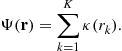 (4.34)
Obviously, we have ![]() . Conversely, this lower bound cannot be achieved in general: assume for instance that
. Conversely, this lower bound cannot be achieved in general: assume for instance that ![]() is reached once: say, the first source. The above lower bound is achieved only if
is reached once: say, the first source. The above lower bound is achieved only if ![]() is the matrix having non-zero components on the first column only. This of course violates the constraint that
is the matrix having non-zero components on the first column only. This of course violates the constraint that ![]() is unitary. We have the following tight result:
is unitary. We have the following tight result:
Proposition 11
As![]() for all the sources, we have, for any unitary
for all the sources, we have, for any unitary![]() :
:
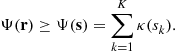 (4.35)
Moreover, the inequality is an equality if and only if![]() essentially equals the identity matrix.
essentially equals the identity matrix.
Proof
By “essentially equal to,” we mean that ![]() is a diagonal matrix with modulus entries, whose columns are permuted. The proof of this result follows the proof of Proposition 3 and was suggested by Common in [2]. We indeed, express
is a diagonal matrix with modulus entries, whose columns are permuted. The proof of this result follows the proof of Proposition 3 and was suggested by Common in [2]. We indeed, express ![]() as
as
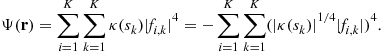
On the other hand, we have the inequality:
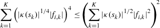
implying that
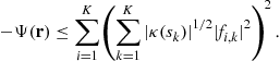 (4.36)
We now denote by ![]() the matrix whose component
the matrix whose component ![]() is
is ![]() and by
and by ![]() so that the r.h.s. of (4.36) is simply
so that the r.h.s. of (4.36) is simply ![]() . As
. As ![]() we deduce that the sum of the elements of any row/column of
we deduce that the sum of the elements of any row/column of ![]() is equal to one:
is equal to one: ![]() is called doubly stochastic. As a consequence of the Birkhoff theorem (see [33] Chapter 2),
is called doubly stochastic. As a consequence of the Birkhoff theorem (see [33] Chapter 2), ![]() can be seen as the convex sum of permutation matrices, i.e.,
can be seen as the convex sum of permutation matrices, i.e., ![]() where, for any index
where, for any index ![]() and
and ![]() . We deduce that
. We deduce that
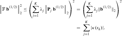
This proves Eq. (4.35). Let us inspect the case of equality. If equality occurs, the inequality (4.36) is necessarily an equality. Hence we have, for any indices i and ![]()
![]()
If all the numbers ![]() are strictly negative, hence non-null, the above conditions implies that, for any index i, the vector
are strictly negative, hence non-null, the above conditions implies that, for any index i, the vector ![]() , i.e., the ith row of the matrix
, i.e., the ith row of the matrix ![]() , has at most one non zero component. On the other hand, the matrix
, has at most one non zero component. On the other hand, the matrix ![]() is unitary. This imposes that
is unitary. This imposes that ![]() essentially equals the identity matrix.
essentially equals the identity matrix. ![]()
In practice, the function ![]() given by Eq. (4.34)cannot be computed. As the data are supposed to be complex-circular at the second-order, we have
given by Eq. (4.34)cannot be computed. As the data are supposed to be complex-circular at the second-order, we have
![]()
A consistent estimate of ![]() is hence
is hence
 (4.37)
The minimization of this function is carried out over the space of unitary matrices. This can be done by using a Jacobi-like algorithm: unitary matrices are parametrized by means of the Given angles. The reader may find details in [2]. Notice that no results concerning the convergence of the algorithm can be said, since it has not been shown that the local minima of the “true” function ![]() are “good ones”, i.e., achieve the BSS.
are “good ones”, i.e., achieve the BSS.
2.04.3.5.2 Generalization: notion of contrast function
We introduce the function
 (4.38)
where ![]() is a function to be specified. Rather than minimizing
is a function to be specified. Rather than minimizing ![]() , we address its maximization. If the maximum is attained when (and only when) BSS is achieved,
, we address its maximization. If the maximum is attained when (and only when) BSS is achieved, ![]() is called a contrast function. As seen previously, the choice
is called a contrast function. As seen previously, the choice ![]() makes
makes ![]() be a contrast function. We have, more generally:
be a contrast function. We have, more generally:
Proposition 12
If![]() is a convex function on
is a convex function on![]() such that
such that![]() and if, for any source index k the condition
and if, for any source index k the condition![]() is fulfilled, then
is fulfilled, then![]() is a contrast function.
is a contrast function.
Proof
For any index i, we have: ![]() . As
. As ![]() is unitary, we deduce that
is unitary, we deduce that ![]() . Hence
. Hence ![]() . We set
. We set ![]() . The Jensen inequality gives here:
. The Jensen inequality gives here:
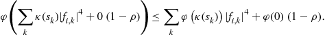
As ![]() , we deduce that
, we deduce that
![]()
By assumption all the ![]() hence the same argument as the one given in the proof of Proposition 11 shows that the maximum is
hence the same argument as the one given in the proof of Proposition 11 shows that the maximum is ![]() and that this maximum is reached if and only if the matrix
and that this maximum is reached if and only if the matrix ![]() is essentially the identity.
is essentially the identity. ![]()
The standard choice for ![]() is
is ![]() . In this case, is enlightening to notice that maximizing
. In this case, is enlightening to notice that maximizing ![]() is equivalent to minimizing:
is equivalent to minimizing:
![]() (4.39)
(4.39)
which is clearly a measure of independence (up to the fourth-order).
2.04.3.5.3 A popular algorithm: JADE
If the indices ![]() are fixed, it may be noticed that the matrix
are fixed, it may be noticed that the matrix ![]() whose entry
whose entry ![]() is given by
is given by ![]() admits the factorization
admits the factorization
![]()
where ![]() is diagonal; the entry
is diagonal; the entry ![]() is
is ![]() . Otherwise stated, U diagonalizes the normal matrix
. Otherwise stated, U diagonalizes the normal matrix ![]() whatever the indices
whatever the indices ![]() . Introducing the
. Introducing the ![]() operator that sums all the entries of a matrix except the ones located on the main diagonal, this says that
operator that sums all the entries of a matrix except the ones located on the main diagonal, this says that
![]() (4.40)
(4.40)
is minimum, equal to zero, when ![]() essentially equals the identity matrix. Conversely, it can be shown that (4.40) can be written as (4.39). Hence a minimizer of the function given in (4.40) is a maximizer of
essentially equals the identity matrix. Conversely, it can be shown that (4.40) can be written as (4.39). Hence a minimizer of the function given in (4.40) is a maximizer of ![]() with
with ![]() . Now, Proposition 12 with the fact that, for any index
. Now, Proposition 12 with the fact that, for any index ![]() proves that the maximizers of
proves that the maximizers of ![]() are such that F is essentially equal to the identity matrix. This trick of algebra allows one to achieve the maximization of
are such that F is essentially equal to the identity matrix. This trick of algebra allows one to achieve the maximization of ![]() thanks to a joint diagonalization of a set of normal matrices. It has been proposed by Cardoso [4] The algorithm associated with this approach is called JADE. It is very popular since efficient algorithms of joint diagonalization are known [20].
thanks to a joint diagonalization of a set of normal matrices. It has been proposed by Cardoso [4] The algorithm associated with this approach is called JADE. It is very popular since efficient algorithms of joint diagonalization are known [20].
Notice that the pencil of matrices is a pencil of normal matrices hence the matrix U is searched in the set of unitary matrices. Recently, Yeredor et al. [34] suggest to relax the unitary constraint. These authors even suggest to skip the pre-whitening of the data: they argue that the pre-whitening may limit the attainable performance as Cardoso pointed it out in [35]. With no whitening of the data, the matrices of cumulants are still jointly diagonalized; if the channel matrix H is square, the columns of this latter form a basis for the diagonalization. The converse is not clear on the one hand and, on the other hand, the case of tall matrices H remains to be addressed.
2.04.3.6 Generalizations
We have presented ad’hoc BSS methods, whose theoretical foundations are solid and whose good performance is well-known. In the literature, however, many other methods can be found. They stem from considerations of information theory. We provide some key ideas and related bibliographical references.
After pre-whitening, we recall that the received data is ![]() (we have dropped the time index): on the one hand, U is unitary and on the other hand, the component of the random variables in s are mutually independent. The idea of independent Component Analysis (ICA) is hence to exhibit matrices V such that the components of
(we have dropped the time index): on the one hand, U is unitary and on the other hand, the component of the random variables in s are mutually independent. The idea of independent Component Analysis (ICA) is hence to exhibit matrices V such that the components of ![]() are “as much independent as possible”. This independency may be measured by the Kullback-Leibler divergence between the distribution of r and this of the product of the marginals: this is the mutual information
are “as much independent as possible”. This independency may be measured by the Kullback-Leibler divergence between the distribution of r and this of the product of the marginals: this is the mutual information ![]() . It is well-known that
. It is well-known that ![]() with equality iff the components of r are independent.
with equality iff the components of r are independent.
Besides, it has been underlined by Comon in [2] that the Darmois theorem states the fact: as the sources are non-Gaussian, the fact that the components of ![]() are pair-wise independent (which is naturally the case if they are mutually independent) implies that
are pair-wise independent (which is naturally the case if they are mutually independent) implies that ![]() is essentially equal to the identity matrix. Hence, the minimization of the mutual information of
is essentially equal to the identity matrix. Hence, the minimization of the mutual information of ![]() is legitimate. This induces of course no BSS algorithm, since the mutual information cannot be simply estimated.
is legitimate. This induces of course no BSS algorithm, since the mutual information cannot be simply estimated.
Now, Comon underlines in the seminal paper [2] that ![]() where
where ![]() is the negentropy of the vector
is the negentropy of the vector ![]() , i.e.,
, i.e., ![]() : here,
: here, ![]() is the differential entropy of
is the differential entropy of ![]() and
and ![]() the differential entropy of the Gaussian vector whose mean and covariance matrix are those of
the differential entropy of the Gaussian vector whose mean and covariance matrix are those of ![]() . The negentropy shows the nice property of invariance w.r.t. any invertible change of variables: hence
. The negentropy shows the nice property of invariance w.r.t. any invertible change of variables: hence ![]() does not depend on
does not depend on ![]() . The independence is then obtained by maximizing
. The independence is then obtained by maximizing
 (4.41)
Notice that ![]() with equality when
with equality when ![]() is Gaussian. Hence the maximization in question tends to maximize the distance of the reconstructed source
is Gaussian. Hence the maximization in question tends to maximize the distance of the reconstructed source ![]() to the Gaussian case.
to the Gaussian case.
On the other hand, this shows that, in order to achieve independency, it suffices to consider the maximization of a sum of functions, each of which simply depends on a component of the reconstructed source vector. Evidently, the maximization of the function ![]() under the constraint that the first row of
under the constraint that the first row of ![]() has norm one, is achieved when
has norm one, is achieved when ![]() coincides with one of the sources up to a modulus one factor. In this respect, this remark provides a justification of the iterative methods proposed in Section 2.04.3.4, even if the function considered are not the negentropy. As far as the function
coincides with one of the sources up to a modulus one factor. In this respect, this remark provides a justification of the iterative methods proposed in Section 2.04.3.4, even if the function considered are not the negentropy. As far as the function ![]() is concerned, notice that it has the form (4.41).
is concerned, notice that it has the form (4.41).
Comon proposes an approximation of the negentropy, based on the Edgeworth expansion of the probability density functions of the random variables ![]() . Thanks to the circularity assumption, this approximation is
. Thanks to the circularity assumption, this approximation is ![]() . This calls for an important remark: the function
. This calls for an important remark: the function ![]() given in Eq. (4.38) with
given in Eq. (4.38) with ![]() is hence closely connected to a measure of independence—this confirms a remark previously done.
is hence closely connected to a measure of independence—this confirms a remark previously done.
Hyvarinen departs from functions based on the cumulants. In [36], it is suggested to consider a wider class of functions which are not directly related to cumulants. In short, the new functions to be maximized are more robust to outliers. The price to be paid is the weaker results concerning the separation: for instance, the precious results concerning the separability of the local maxima do not hold. An efficient algorithm has given rise to the popular method called FastICA. In the original paper [36], the sources are real valued which is not the case in this paper. An extension to complex-valued sources can be found in [3].
2.04.3.7 Iterative BSS (general cyclo-stationary case)
We specified that the assumption of stationarity of the sources, as required in the previous sections, is somewhat restrictive in a realistic scenario of telecommunication. Indeed, the stationarity implicitly assumes that all the sources have the same symbol period and that the data are sampled at a period equal to the symbol period. In general—think for instance of a passive listening context—the sources have different baud-rates. We denote the symbol periods of the K sources by ![]() . If
. If ![]() is the sampling period—a priori different of any of the symbol periods—we have deduce from Section 2.04.2 that, for any index k, the source
is the sampling period—a priori different of any of the symbol periods—we have deduce from Section 2.04.2 that, for any index k, the source ![]() is cyclostationary. In particular, the second moment
is cyclostationary. In particular, the second moment ![]() varies with the time-index n. More specifically, we have
varies with the time-index n. More specifically, we have
![]()
where
![]()
is the set of the second-order cyclic frequencies of ![]() and the Fourier coefficients
and the Fourier coefficients ![]() are given by Eq. (4.8) (we have dropped the time-lag in
are given by Eq. (4.8) (we have dropped the time-lag in ![]() since, in the sequel, no other time delay than
since, in the sequel, no other time delay than ![]() is considered). In this section, the channel is supposed to be memoryless, as in all the Section 2.04.3. Hence, the model given by Eq. (4.11) still holds: the components of the source vector
is considered). In this section, the channel is supposed to be memoryless, as in all the Section 2.04.3. Hence, the model given by Eq. (4.11) still holds: the components of the source vector ![]() are effectively mutually independent, but are not individually stationary. As far as the normalization of the sources is concerned, it may also be assumed: in the cyclo-stationary context of this section, this means that
are effectively mutually independent, but are not individually stationary. As far as the normalization of the sources is concerned, it may also be assumed: in the cyclo-stationary context of this section, this means that
![]() (4.42)
(4.42)
In the following, we provide assumptions on the sources that guarantee that the algorithms of source separation depicted in Section 2.04.3.4 still converge to desirable solutions, i.e., allow one to separate the sources. In other words, the algorithms previously considered are run as if the data were stationary: this means that nothing has to be changed in any part of the stationary BSS algorithms. Surprisingly, the fact that the data are not stationary is shown not to impact the convergence to a good (separating) solution.
The algorithms encountered for stationary data (see Section 2.04.3.4) are designed to minimize either the function ![]() given by Eq. (4.31) or the Godard function
given by Eq. (4.31) or the Godard function ![]() given by Eq. (4.32). Let us recall that the signal
given by Eq. (4.32). Let us recall that the signal ![]() is the output of the variable spatial filter
is the output of the variable spatial filter ![]() , i.e.,
, i.e.,
![]()
where ![]() . As in the stationary case, we analyze the argument minima of the theoretical associated function. The first point to be addressed is hence: to which functions
. As in the stationary case, we analyze the argument minima of the theoretical associated function. The first point to be addressed is hence: to which functions ![]() and
and ![]() converge? Due to the non-stationarity of the model, the function
converge? Due to the non-stationarity of the model, the function ![]() for instance does not converge to
for instance does not converge to ![]() as given in Eq. (4.30): this cannot be the case since the latter function depends on the time-lag n.
as given in Eq. (4.30): this cannot be the case since the latter function depends on the time-lag n.
There is a version of the law of the large numbers for non-stationary data. Lemma 8 can be written in this context under this form:
Lemma 13
For![]() , we have, with probability one:
, we have, with probability one:
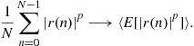
We deduce that ![]() . We define this limit as (the superscript “c” means “cyclo-stationary”):
. We define this limit as (the superscript “c” means “cyclo-stationary”):
![]() (4.43)
(4.43)
For the same reason, we have ![]() where
where
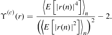 (4.44)
Notice that, in the case of stationary data, ![]() (respectively
(respectively ![]() ) equals
) equals ![]() (respectively
(respectively ![]() ).
).
We first address the minimization of ![]() . Once done, we deduce results concerning the minimization of
. Once done, we deduce results concerning the minimization of ![]() .
.
We consider a prior expansion of the moments involved in ![]() . The following equality always holds true (we recall that the signals are all complex-circular at the second-order):
. The following equality always holds true (we recall that the signals are all complex-circular at the second-order):
![]() (4.45)
(4.45)
The multi-linearity of the cumulant gives:
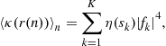
where we let for any source ![]() the number
the number ![]() be
be
![]() (4.46)
(4.46)
The output of the spatial filter, ![]() , is obviously a linear combination of the sources
, is obviously a linear combination of the sources ![]() . As
. As ![]() admits
admits ![]() as the set of its second-order cyclic frequencies, we deduce that
as the set of its second-order cyclic frequencies, we deduce that ![]() is cyclo-stationary and its second-order cyclo-frequencies are in the set
is cyclo-stationary and its second-order cyclo-frequencies are in the set

This means that ![]() . As a consequence, the term
. As a consequence, the term ![]() , may be computed thanks to the Parseval equality. We have indeed
, may be computed thanks to the Parseval equality. We have indeed
![]()
On the other hand, the sources are mutually decorrelated hence
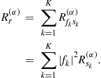
By definition, ![]() is the set of all the non-null cyclic frequencies of the mixture. After isolating the term associated with the cyclic frequency
is the set of all the non-null cyclic frequencies of the mixture. After isolating the term associated with the cyclic frequency ![]() , we may hence write that
, we may hence write that

where
![]() (4.47)
(4.47)
We have used the symmetry:
![]() (4.48)
(4.48)
The set ![]() is simply
is simply ![]() . Denoting by
. Denoting by ![]() the set
the set ![]() we have, due to (4.48), the alternative expression of
we have, due to (4.48), the alternative expression of ![]() that underlines that
that underlines that ![]() is real:
is real:
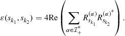 (4.49)
We hence have the following expression:
 (4.50)
where we have let, for any of the sources ![]() whose positive cyclic frequency is
whose positive cyclic frequency is ![]() the number
the number ![]() be
be
![]() (4.51)
(4.51)
It is to be noticed that ![]() can also be expressed as
can also be expressed as
![]() (4.52)
(4.52)
We are in position to discuss the minimization of this function. Two cases have to be distinguished.
2.04.3.7.1 Case of different baud-rates
If the cyclic frequencies ![]() are all different modulo 1, the coefficients
are all different modulo 1, the coefficients ![]() all verify:
all verify:
![]() (4.53)
(4.53)
Indeed, it suffices to consider the expression of Eq. (4.47): let ![]() be the positive cyclo-frequency of the source no
be the positive cyclo-frequency of the source no ![]() . In Eq. (4.47), there are at most two terms:
. In Eq. (4.47), there are at most two terms: ![]() is either
is either ![]() or
or ![]() modulo 1. Take for instance
modulo 1. Take for instance ![]() . The associated term is non null if
. The associated term is non null if ![]() or
or ![]() : if
: if ![]() and
and ![]() are different modulo 1, this cannot occur. The same reasoning applies for
are different modulo 1, this cannot occur. The same reasoning applies for ![]() . In other words,
. In other words, ![]() .
.
Remark
It is desirable to bridge the gap between this condition on the disparity of the cyclo-frequencies and practical considerations. We insist on the fact that the above condition is not equivalent to condition that the symbol frequencies are different. Indeed, consider ![]() and
and ![]() . Then
. Then ![]() modulo 1 and the condition is not fulfilled whereas the symbol periods are different. However, if the sampling frequency is big enough such that for all indices
modulo 1 and the condition is not fulfilled whereas the symbol periods are different. However, if the sampling frequency is big enough such that for all indices ![]() then the condition on the disparity of the cyclic frequencies simply means: all the symbol periods are different. In the following, we systematically assume the condition
then the condition on the disparity of the cyclic frequencies simply means: all the symbol periods are different. In the following, we systematically assume the condition
![]() (4.54)
(4.54)
Proposition 3 can be written in the non-stationary context:
Proposition 14
If the cyclic frequencies![]() are all different modulo
are all different modulo![]() then the cost function
then the cost function![]() achieves its minimum at a separating vector if and only if one of the
achieves its minimum at a separating vector if and only if one of the![]() is strictly negative. Moreover, the separating vector in question has its single non-null element located at an index
is strictly negative. Moreover, the separating vector in question has its single non-null element located at an index![]() such that
such that![]() .
.
We hence consider the following assumption
![]() (4.55)
(4.55)
that is analyzed in Section 2.04.3.9.
Together with Proposition 14, this assumption ![]() allows one to claim that the minimization of the estimated function
allows one to claim that the minimization of the estimated function ![]() is legitimate as far as the extraction of a source is concerned. Moreover, the result of Lemma 5 still holds: indeed, the expression of
is legitimate as far as the extraction of a source is concerned. Moreover, the result of Lemma 5 still holds: indeed, the expression of ![]() given by (4.50) simplifies as
given by (4.50) simplifies as
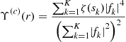
which is formally the same as the function ![]() considered in the stationary case—see Eq. (4.29). The local minima of
considered in the stationary case—see Eq. (4.29). The local minima of ![]() are separating, which makes the minimization algorithm based on a gradient method robust to the presence of local minima.
are separating, which makes the minimization algorithm based on a gradient method robust to the presence of local minima.
We now face the minimization of the function ![]() . The question is whether the non-stationarity of the data changes such a result as the one given in Proposition 7 or not. The careful reader will be assured that indeed Proposition 7 is true in the non-stationary case. Moreover, the result of Proposition 4 is unchanged in the cyclo-stationary case. We can claim:
. The question is whether the non-stationarity of the data changes such a result as the one given in Proposition 7 or not. The careful reader will be assured that indeed Proposition 7 is true in the non-stationary case. Moreover, the result of Proposition 4 is unchanged in the cyclo-stationary case. We can claim:
Proposition 15
If the cyclic frequencies![]() are all different modulo
are all different modulo![]() and if Assumption
and if Assumption![]() in (4.55) holds, then the local minima of the cost functions
in (4.55) holds, then the local minima of the cost functions![]() and
and![]() are separating.
are separating.
2.04.3.7.2 General case
Contrary to the case where the cyclic-frequencies are different, the Eq. (4.53) does not hold in general, and the results given in the stationary context concerning the minimization of ![]() cannot be directly recast. However, numerical considerations may help to give similar results. In this respect, the reader should understand that the quantities
cannot be directly recast. However, numerical considerations may help to give similar results. In this respect, the reader should understand that the quantities ![]() are either zero or “small” since they involve cyclo-correlation at non-null frequencies. This is specific of telecommunication signals; the reason is due to the fact that the excess bandwidth of a transmitted signal is small (see [37]). We will discuss this fact further on, but for the moment, we simply consider the following assumption for any of the sources, denoted by s:
are either zero or “small” since they involve cyclo-correlation at non-null frequencies. This is specific of telecommunication signals; the reason is due to the fact that the excess bandwidth of a transmitted signal is small (see [37]). We will discuss this fact further on, but for the moment, we simply consider the following assumption for any of the sources, denoted by s:
![]() (4.56)
(4.56)
We discuss this assumption further in Section 2.04.3.9. For the moment, we suppose that Assumptions ![]() and
and ![]() both hold.
both hold.
Consider two distinct indices ![]() and
and ![]() ; for sake of simplicity, let them be
; for sake of simplicity, let them be ![]() and
and ![]() . Notice that if the sources numbered 1 and 2 are such that their associated (single) cyclic frequencies are different modulo 1 then
. Notice that if the sources numbered 1 and 2 are such that their associated (single) cyclic frequencies are different modulo 1 then ![]() . Suppose on the contrary now that the cyclic frequencies are equal modulo 1 (thanks to (4.54) this happens if and only if the two baud-rates are the same). In this case, the summation (4.49) has only one term and
. Suppose on the contrary now that the cyclic frequencies are equal modulo 1 (thanks to (4.54) this happens if and only if the two baud-rates are the same). In this case, the summation (4.49) has only one term and ![]() . Assumption
. Assumption ![]() given in (4.56) holds, it follows in both cases that
given in (4.56) holds, it follows in both cases that ![]() . Whatever the indices
. Whatever the indices ![]() may be, Assumption
may be, Assumption ![]() implies
implies
![]() (4.57)
(4.57)
We may consider the expression of ![]() given in Eq. (4.50). We have, thanks to (4.57):
given in Eq. (4.50). We have, thanks to (4.57):
 (4.58)
As the r.h.s of the latter equation is simply ![]() , this shows that
, this shows that

If Assumption ![]() holds, this lower bound is evidently reached. It remains to inspect the cases of equality for this lower-bound. In this respect, we suppose that
holds, this lower bound is evidently reached. It remains to inspect the cases of equality for this lower-bound. In this respect, we suppose that ![]() where
where ![]() . For convenience, we assume that
. For convenience, we assume that ![]() . The case of equality implies that (4.58) is an equality. It implies that
. The case of equality implies that (4.58) is an equality. It implies that
![]()
Now, the inequality ![]() implies that
implies that ![]() . Necessarily, we must have that, for every couples
. Necessarily, we must have that, for every couples ![]() such that
such that ![]() . Otherwise stated: the vector
. Otherwise stated: the vector ![]() has a single non-null component, hence is separating.
has a single non-null component, hence is separating.
We have shown the result:
Proposition 16
If the Assumptions![]() and
and![]() hold, then the cost function
hold, then the cost function![]() and
and![]() achieve their minimum at a separating vector.
achieve their minimum at a separating vector.
2.04.3.8 Global BSS (general cyclo-stationary case)
Again in this section, the global source separation method depicted in Section 2.04.3.5 is considered. Its convergence was specifically shown for stationary sources. We show that the convergence of the algorithm to a separating matrix is not affected when the data are cyclo-stationary. This key-result was first provided in [38]; a condition of separability of JADE was given, which was rather difficult to interpret especially when the number of sources is greater than 3. We show the result quite differently, following [39].
Notice that the pre-whitening of the observed data is still possible even when the data are cyclo-stationary: the algorithm is even not changed at all. Hence, we begin by considering the estimate ![]() given by Eq. (4.37). Obviously, this estimate can not converge to the function of the cumulants given by Eq. (4.34) since the terms in this equation depend on the time lag. Nevertheless, the limit as the number of snapshots grows can be expressed as
given by Eq. (4.37). Obviously, this estimate can not converge to the function of the cumulants given by Eq. (4.34) since the terms in this equation depend on the time lag. Nevertheless, the limit as the number of snapshots grows can be expressed as
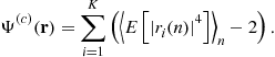
Thanks to the algebra already done along Section 2.04.3.7, we may directly write
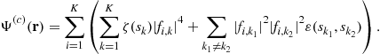
It remains little to do as soon as Assumptions ![]() and
and ![]() hold, since the following inequality holds:
hold, since the following inequality holds:

where ![]() . The same argument as the one given in Section 2.04.3.5 (Birkhoff theorem) proves that
. The same argument as the one given in Section 2.04.3.5 (Birkhoff theorem) proves that ![]() . As the numbers
. As the numbers ![]() , thanks to Assumption
, thanks to Assumption ![]() , are strictly negative, we directly show that
, are strictly negative, we directly show that ![]() is the infimum of
is the infimum of ![]() and this infimum is reached for unitary matrices
and this infimum is reached for unitary matrices ![]() that are essentially equal to the identity matrix. This proves the following proposition, that is the sister of Proposition 11:
that are essentially equal to the identity matrix. This proves the following proposition, that is the sister of Proposition 11:
Proposition 17
If Assumptions![]() and
and![]() hold, we have, for any unitary
hold, we have, for any unitary![]() :
:
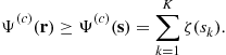
Moreover, the inequality is an equality if and only if![]() essentially equals the identity matrix.
essentially equals the identity matrix.
2.04.3.9 Validity of assumptions  and
and  : semi-analytical considerations
In essence, we have shown that the cyclo-stationarity of the data does not affect neither the one-by-one methods of Section 2.04.3.7, nor the global method depicted in Section 2.04.3.5. This positive answer to our question however requires to inspect the validity of Assumptions ![]() and
and ![]() . We first discuss
. We first discuss ![]() . We recall that, in a stationary environment,
. We recall that, in a stationary environment, ![]() is simply the fourth-order cumulant of the (normalized) source. As this latter is a filtered version of an i.i.d. sequence of symbols having a strictly negative Kurtosis, it is straight-forward that
is simply the fourth-order cumulant of the (normalized) source. As this latter is a filtered version of an i.i.d. sequence of symbols having a strictly negative Kurtosis, it is straight-forward that ![]() . In a cyclo-stationary environment, the mentioned argument does not hold anymore. In this case, indeed,
. In a cyclo-stationary environment, the mentioned argument does not hold anymore. In this case, indeed, ![]() is given by (4.51) and it is not possible to conclude directly that
is given by (4.51) and it is not possible to conclude directly that ![]() . However, these statistics can be shown to express as integrals of the shaping filter
. However, these statistics can be shown to express as integrals of the shaping filter ![]() , at least for a generic sampling frequency (see [40]). More precisely, except for four sampling frequencies that are irrelevant to consider, it can be shown quite simply that
, at least for a generic sampling frequency (see [40]). More precisely, except for four sampling frequencies that are irrelevant to consider, it can be shown quite simply that
![]()
and
![]()
where ![]() , as specified in the introduction, is a normalized square-root raised-cosine filter. In [40], it is shown rigorously that
, as specified in the introduction, is a normalized square-root raised-cosine filter. In [40], it is shown rigorously that ![]() and
and ![]() do not depend on the symbol period T. It is hence possible to compute numerically
do not depend on the symbol period T. It is hence possible to compute numerically ![]() as a function of the excess bandwidth, while considering a few values of
as a function of the excess bandwidth, while considering a few values of ![]() corresponding to typical modulations. The reader may find details on the computation of these numbers in the above reference. The results are reported in Figure 4.7. In order to validate that the above formulas are correct, we also have plotted the estimate of
corresponding to typical modulations. The reader may find details on the computation of these numbers in the above reference. The results are reported in Figure 4.7. In order to validate that the above formulas are correct, we also have plotted the estimate of ![]() obtained by stochastic simulations with respect to Eq. (4.52) (we have generated sequences of 10,000 symbols according to the modulation). For all the values of the excess bandwidth, the numerical results let us claim that
obtained by stochastic simulations with respect to Eq. (4.52) (we have generated sequences of 10,000 symbols according to the modulation). For all the values of the excess bandwidth, the numerical results let us claim that ![]() is true.
is true.

At a first sight, Assumption ![]() looks quite audacious; indeed it is. As far as we know, it is not possible, for the same reasons as those mentioned above, to prove this result analytically. Resorting again to semi-analytical considerations, we compute the numbers
looks quite audacious; indeed it is. As far as we know, it is not possible, for the same reasons as those mentioned above, to prove this result analytically. Resorting again to semi-analytical considerations, we compute the numbers ![]() and
and ![]() for different modulations and excess-bandwidth factors. We have obtained the results that can be seen in Figure 4.8. These computations indicate that
for different modulations and excess-bandwidth factors. We have obtained the results that can be seen in Figure 4.8. These computations indicate that ![]() can be claimed to hold.
can be claimed to hold.
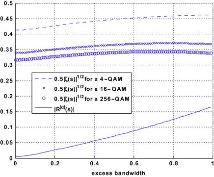
2.04.4 Convolutive mixtures: case of sparse channels
We now face the problem of blind source separation when the channel is not memoryless. The contribution of a given source to received data is not simply the delayed source up to an unknown constant, but a filtered version of the source. In this section, we specify the model and we explain how it is possible to connect quite directly the previous results (on instantaneous mixtures) to this model: this requires a strong assumption on the delays as will be explained. We refer to [41] (Chapter 17) for more details.
The convolutive effect stems from the presence of multiple paths as specified in Section 2.04.2.1. Consider a source ![]() ; the contribution of this source on the received signal (mth sensor) is given by (4.9). In most of the high-rate digital communication systems, the narrow-band assumption may be taken for granted. By narrow-band signal, we mean that the carrier frequency is big enough to consider the signal as monochromatic. More specifically, this means that the bandwidth of the signal in baseband is much smaller than the carrier frequency, i.e.,
; the contribution of this source on the received signal (mth sensor) is given by (4.9). In most of the high-rate digital communication systems, the narrow-band assumption may be taken for granted. By narrow-band signal, we mean that the carrier frequency is big enough to consider the signal as monochromatic. More specifically, this means that the bandwidth of the signal in baseband is much smaller than the carrier frequency, i.e.,
![]()
On the other hand, for any delay ![]() such that
such that ![]() , we have the approximation:
, we have the approximation: ![]() . In order to take the full benefit of the antenna array, the distance between two consecutive antennas should be of the order of half the wave-length. This says that the delay of propagation between two consecutive antennas is of the order of
. In order to take the full benefit of the antenna array, the distance between two consecutive antennas should be of the order of half the wave-length. This says that the delay of propagation between two consecutive antennas is of the order of ![]() . As a consequence, the contribution of the kth source and
. As a consequence, the contribution of the kth source and ![]() th path to the mixture is a rank one signal and can be written as
th path to the mixture is a rank one signal and can be written as ![]() where
where ![]() is called steering vector.
is called steering vector.
We assume that the associated delays are sorted such that ![]() We consider the case when the delays are “sufficiently spread out.” In this respect, the reader should notice that it is possible to use the fact that the shaping function
We consider the case when the delays are “sufficiently spread out.” In this respect, the reader should notice that it is possible to use the fact that the shaping function ![]() numerically vanishes:
numerically vanishes: ![]() can be numerically neglected if
can be numerically neglected if ![]() where the integer
where the integer ![]() depends on the roll-off. This implies that
depends on the roll-off. This implies that

Consider that the above approximation is an equality. As a consequence, if ![]() then the random variables
then the random variables ![]() and
and ![]() do not involve the same symbols hence they are independent. Two consecutive paths can hence be treated as independent sources. Suppose that all the successive delays are separated by more than
do not involve the same symbols hence they are independent. Two consecutive paths can hence be treated as independent sources. Suppose that all the successive delays are separated by more than ![]() , this property holding true for all the sources. As
, this property holding true for all the sources. As ![]() denotes the number of paths associated with the kth source, we may write the observed data according to Eq. (4.11). This time, the “source vector”
denotes the number of paths associated with the kth source, we may write the observed data according to Eq. (4.11). This time, the “source vector” ![]() is defined as
is defined as
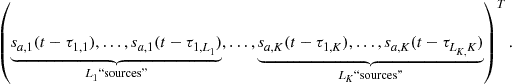
The ![]() “sources” in the vector
“sources” in the vector ![]() are (approximately) mutually independent. The advantage of this formulation is that all the results given in Section 2.04.3.7 remain true. Nevertheless, we want to stress the drawbacks of this approach.
are (approximately) mutually independent. The advantage of this formulation is that all the results given in Section 2.04.3.7 remain true. Nevertheless, we want to stress the drawbacks of this approach.
1. A fundamental requirement is that the number of sensors, M, is greater than the number of sources. We recall that this necessary condition comes from the requirement that the mixing matrix H should have full -column rank. This gives here
![]()
This condition may be limiting as soon as the number of paths per communication source is big.
2. The source separation methods all require that the components of ![]() be mutually independent. Now, the delays are spread out in very specific conditions; this particular consition occurs in long-range communication channels (ionospheric transmissions): we refer to the reference [41] (Chapter 17) for details. On the contrary, this assumption on the distribution of the delays associated with a given source is scarcely fulfilled in many cases (urban GSM channels for instance).
be mutually independent. Now, the delays are spread out in very specific conditions; this particular consition occurs in long-range communication channels (ionospheric transmissions): we refer to the reference [41] (Chapter 17) for details. On the contrary, this assumption on the distribution of the delays associated with a given source is scarcely fulfilled in many cases (urban GSM channels for instance).
3. The complexity of the instantaneous (one-by-one or global) methods directly increases with the number of sources.
4. The algorithms of source separation, ideally, should provide, up to constants, all the components of ![]() . For instance,
. For instance, ![]() of these “sources” among the
of these “sources” among the ![]() components involve the sequence of symbols
components involve the sequence of symbols ![]() . As the ultimate goal is to eventually estimate these transmitted symbols, a recombination of the
. As the ultimate goal is to eventually estimate these transmitted symbols, a recombination of the ![]() “sources” has to be computed. Notice that the sources are generally not ordered in any way. The association of th e reconstructed paths can be processed after lagged correlation between the reconstructed sources. This is clearly not a child’s play.
“sources” has to be computed. Notice that the sources are generally not ordered in any way. The association of th e reconstructed paths can be processed after lagged correlation between the reconstructed sources. This is clearly not a child’s play.
For practical considerations, we refer to Chapter 17 of reference [41] where a comparison between instantaneous (described in this section) and convolutive approaches described in the next section are done.
2.04.5 Convolutive mixtures
We now face the case of the general multi-path channels; no such condition as the sparsity of the channels is assumed to hold.
2.04.5.1 Identifying the symbols: algebraic methods (stationary data)
In this section, the model of the data is stationary and is given by (4.18). We have justified in the introduction that it is legitimate to approximate the MIMO filter ![]() by a polynomial. We denote by L its order, i.e.,
by a polynomial. We denote by L its order, i.e.,
![]() . The approaches that we want to introduce exploit algebraic properties of the model (convolution) and of the source signal
. The approaches that we want to introduce exploit algebraic properties of the model (convolution) and of the source signal ![]() . Van der Veen et al. [42] suggest the following method.
. Van der Veen et al. [42] suggest the following method.
Consider the vector
![]() (4.59)
(4.59)
for ![]() . We remark that
. We remark that
![]()
where ![]() is defined in the same manner as
is defined in the same manner as ![]() and where matrix
and where matrix ![]() is the
is the ![]() block-Toeplitz matrix given by
block-Toeplitz matrix given by
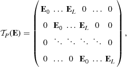 (4.60)
where we have set ![]() . Denote by
. Denote by ![]() the
the ![]() matrix (N is the number of snapshots) in which all the data
matrix (N is the number of snapshots) in which all the data ![]() from
from ![]() to
to ![]() are collected (
are collected (![]() ): the n th column of
): the n th column of ![]() is
is ![]() —see (4.59). It yields
—see (4.59). It yields ![]() where
where ![]() is the block-Toeplitz matrix defined by
is the block-Toeplitz matrix defined by

It is known (see [13,43]) that the assumption given in (4.21) involves that ![]() is a full column rank matrix. We deduce that the row space of
is a full column rank matrix. We deduce that the row space of ![]() equals the row space of
equals the row space of ![]() . An idea consists in finding the matrices
. An idea consists in finding the matrices ![]() having the Toeplitz structure of
having the Toeplitz structure of ![]() such that their row space is prescribed. Notice that an ambiguity arises since the estimated
such that their row space is prescribed. Notice that an ambiguity arises since the estimated ![]() of
of ![]() coincide up to an invertible matrix. This latter can be removed by considering one of the algebraic methods (instantaneous mixtures) evoked in Section 2.04.3.2 in which a priori information on the symbols is exploited (finite alphabets or constant modulus modulations).
coincide up to an invertible matrix. This latter can be removed by considering one of the algebraic methods (instantaneous mixtures) evoked in Section 2.04.3.2 in which a priori information on the symbols is exploited (finite alphabets or constant modulus modulations).
2.04.5.2 Estimation of the channels: MA/AR structures (stationary data)
Again in this section, the data are stationary and follow the model (4.18), so that ![]() appears to be a moving average model driven by non-Gaussian i.i.d. sequences. A number of blind identification methods of MA models using higher statistics have been derived, and could be used in the present context (see e.g., [44]). However, the corresponding algorithms show poor performance.
appears to be a moving average model driven by non-Gaussian i.i.d. sequences. A number of blind identification methods of MA models using higher statistics have been derived, and could be used in the present context (see e.g., [44]). However, the corresponding algorithms show poor performance.
If ![]() is irreducible—see (4.21)—there exists a left polynomial inverse of
is irreducible—see (4.21)—there exists a left polynomial inverse of ![]() [43]—say
[43]—say ![]() . This implies that
. This implies that ![]() where
where ![]() is i.i.d., which says that
is i.i.d., which says that ![]() is an AR model. This can be used in order to identify the matrix
is an AR model. This can be used in order to identify the matrix ![]() thanks to a linear prediction approach, and hence to retrieve the symbol sequences [45] up to a constant
thanks to a linear prediction approach, and hence to retrieve the symbol sequences [45] up to a constant ![]() matrix. We note however that the irreducibility of
matrix. We note however that the irreducibility of ![]() does not hold when the excess band-width are all zero due to the factorization evoked at the end of Section 2.04.2.3.2. This tends to indicate a certain lack of robustness of the linear prediction method when the excess bandwidth factors are small.
does not hold when the excess band-width are all zero due to the factorization evoked at the end of Section 2.04.2.3.2. This tends to indicate a certain lack of robustness of the linear prediction method when the excess bandwidth factors are small.
2.04.5.3 Estimation of the channels: subpace methods (cyclo-stationary data)
In the previous sections, the main assumption is that the data are stationary. Here, we rather consider the general model (4.17). We consider here the general cyclo-stationary model.
In order to achieve BSS, it is suggested here to identify the transfer function ![]() , and then to evaluate one of its left inverse in order to retrieve the source signals (this kind of approaches is sometimes called indirect). In this respect,
, and then to evaluate one of its left inverse in order to retrieve the source signals (this kind of approaches is sometimes called indirect). In this respect, ![]() is usually modeled as a FIR causal filter, i.e.,
is usually modeled as a FIR causal filter, i.e., ![]() . It has been shown in [43] that if
. It has been shown in [43] that if ![]() and
and ![]() is full column rank, then
is full column rank, then ![]() can be identified from the column space of
can be identified from the column space of ![]() up to a constant
up to a constant ![]() matrix which can itself be estimated using any instantaneous mixture blind source separation method. In practice, the column space of
matrix which can itself be estimated using any instantaneous mixture blind source separation method. In practice, the column space of ![]() is usually estimated by means of the eigenvalue/ eigenvector decomposition of an estimate of the covariance matrix of vector
is usually estimated by means of the eigenvalue/ eigenvector decomposition of an estimate of the covariance matrix of vector ![]() given in (4.59). We should perhaps specify this point. Indeed, we have
given in (4.59). We should perhaps specify this point. Indeed, we have

where ![]() . If this latter is full rank, the column space of
. If this latter is full rank, the column space of ![]() coincides with the column space of
coincides with the column space of ![]() . However, it should be emphasized that it is not always legitimate to assume that
. However, it should be emphasized that it is not always legitimate to assume that ![]() is full rank except when all the sources occupy all the band of frequencies
is full rank except when all the sources occupy all the band of frequencies ![]() . On the contrary, the rank of
. On the contrary, the rank of ![]() is expected to fall. We do not provide the details: the reader should compute the limit of
is expected to fall. We do not provide the details: the reader should compute the limit of ![]() as
as ![]() and show that the limit
and show that the limit ![]() is a block Toeplitz matrix whose block
is a block Toeplitz matrix whose block ![]() has the expression:
has the expression:
![]()
where ![]() is the (diagonal) power spectral density of the vector
is the (diagonal) power spectral density of the vector ![]() . As the sampling period verifies the Shannon sampling condition, some of the entries of
. As the sampling period verifies the Shannon sampling condition, some of the entries of ![]() are band-limited, which prevents the rank of
are band-limited, which prevents the rank of ![]() from being full (see the works of Slepian and Pollak on the prolate spheroidal wave functions).
from being full (see the works of Slepian and Pollak on the prolate spheroidal wave functions).
Further refinements are proposed in [12]. Notice that this subspace method, although apparently quite appealing, performs poorly as soon as the matrix ![]() is ill-conditioned, which, in practice, is quite often the case.
is ill-conditioned, which, in practice, is quite often the case.
2.04.5.4 Global BSS approaches
2.04.5.4.1 Temporal approaches: extensions of the Comon contrast function (stationary data)
We now focus on the direct and global BSS methods, i.e., methods that allow one to compute a global separator in one shot (up to indeterminacies that will be specified). In this respect, we intend to provide extensions of the approaches given for the instantaneous context—see Section 2.04.3.5. For simplification, assume the (restrictive) stationary case. As specified in the previous paragraph, the model of the data is not stricto sensu ![]() as in Eq. (4.17) since the Shannon sampling condition does not hold, but rather (4.18).
as in Eq. (4.17) since the Shannon sampling condition does not hold, but rather (4.18).
On the one hand, a direct extension of a contrast as defined by Comon can be done (see Section 8.4.2 of [41]). The first step to be considered is the decorrelation of the data (the prewhitening), i.e., a filter matrix ![]() is computed such that
is computed such that ![]() is decorrelated both spatially and temporally. This is equivalent to computing
is decorrelated both spatially and temporally. This is equivalent to computing ![]() such that
such that ![]() is para-unitary, i.e.,
is para-unitary, i.e., ![]() verifies for any frequency
verifies for any frequency ![]() :
: ![]() . The reader may find details of this procedure in [46,47]. The reconstructed vector of the sources may hence be searched as
. The reader may find details of this procedure in [46,47]. The reconstructed vector of the sources may hence be searched as ![]() where
where ![]() is a para-unitary matrix. It is possible to consider, as in the instantaneous case, the function
is a para-unitary matrix. It is possible to consider, as in the instantaneous case, the function
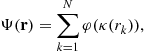
where ![]() shows the same properties as in Proposition 12. It can be simply shown that
shows the same properties as in Proposition 12. It can be simply shown that ![]() , as a function of the para-unitary matrix
, as a function of the para-unitary matrix ![]() , is a contrast, i.e., achieves its maximum for separating matrices
, is a contrast, i.e., achieves its maximum for separating matrices ![]() : see [48]. Theoretically appealing (at least in a stationary environment), this solution calls for implicit prerequisites, namely the pre-whitening and the optimization over the set of para-unitary matrices. Concerning this latter point, solutions have been given (see [10,49]); Comon et al. also suggested to consider a subset of the set of the para-unitary matrices [50]. The solutions are not simple. Besides, the algorithms might be trapped in local maxima.
: see [48]. Theoretically appealing (at least in a stationary environment), this solution calls for implicit prerequisites, namely the pre-whitening and the optimization over the set of para-unitary matrices. Concerning this latter point, solutions have been given (see [10,49]); Comon et al. also suggested to consider a subset of the set of the para-unitary matrices [50]. The solutions are not simple. Besides, the algorithms might be trapped in local maxima.
2.04.5.4.2 Frequency-domain approaches
In the case of stationary data (same restrictive context as in the above subsection), it is possible to recast the results of the instantaneous case after processing the discrete Fourier transform of the data: the separation in processed at each frequency. The difficulty is that the indeterminacies change from a frequency to the other which makes the approach quite difficult. The reader may find references in [51].
Assuming now the general cyclo-stationary model given by (4.17), one may focus on second-order methods. The power spectrum of the data, defined as the discrete Fourier transform of the correlation function at the null cyclic frequency ![]() can be written as
can be written as
![]() (4.61)
(4.61)
where ![]() is the
is the ![]() power spectrum of the source vector given by (4.10). The components of
power spectrum of the source vector given by (4.10). The components of ![]() being jointly independent, hence decorrelated, the matrices
being jointly independent, hence decorrelated, the matrices ![]() are diagonal. As far as the identifiability of the unknown
are diagonal. As far as the identifiability of the unknown ![]() based on the relation (4.61) is addressed, it is shown in [52] that the conditions required are that (4.20) holds on the one hand and, on the other hand, that spectral diversity occurs namely that the entries of
based on the relation (4.61) is addressed, it is shown in [52] that the conditions required are that (4.20) holds on the one hand and, on the other hand, that spectral diversity occurs namely that the entries of ![]() are all distinct for every frequency. In [53,54] its is shown that the matrices
are all distinct for every frequency. In [53,54] its is shown that the matrices ![]() such that
such that ![]() is diagonal for all the frequencies
is diagonal for all the frequencies ![]() are separating matrices. Criteria measuring the closeness to diagonal matrices have been proposed. See also [55] and the references therein. Again, the diversity of the spectra is not always pertinent for digital communication contexts.
are separating matrices. Criteria measuring the closeness to diagonal matrices have been proposed. See also [55] and the references therein. Again, the diversity of the spectra is not always pertinent for digital communication contexts.
2.04.5.5 Iterative BSS (stationary case)
Instead of considering a simple spatial filtering of the data as indicated in Eq. (4.24) we rather process a spatio-temporal filtering as depicted below:
![]() (4.62)
(4.62)
The “reconstructed source” ![]() can be expanded as
can be expanded as
 (4.63)
where the ![]() are components of the global filter
are components of the global filter
![]() (4.64)
(4.64)
A key trick for the following results is the normalization step: we might write ![]() where
where ![]() and
and
![]() (4.65)
(4.65)
Notice that the separation is achieved if and only if the real-valued vector ![]() is separating in the sense given in Section 2.04.3.4. As a consequence, when the separation is achieved, the “reconstructed source” is one of the sources up to a filter with unit norm.
is separating in the sense given in Section 2.04.3.4. As a consequence, when the separation is achieved, the “reconstructed source” is one of the sources up to a filter with unit norm.
With no modification as compared to the method given for the instantaneous case in 2.04.3.4, we consider the optimization of the function ![]() as given in Eq. (4.27)—or equivalently (4.28). For sake of simplicity, we keep the notation
as given in Eq. (4.27)—or equivalently (4.28). For sake of simplicity, we keep the notation ![]() and
and ![]() even if it should be understood that the functions in question depend on the filters
even if it should be understood that the functions in question depend on the filters![]() . No extra computation is needed as compared to the instantaneous case: indeed, it suffices to substitute the “new source”
. No extra computation is needed as compared to the instantaneous case: indeed, it suffices to substitute the “new source” ![]() to the actual source
to the actual source ![]() : one arrives at the expression:
: one arrives at the expression:

This time, the cumulants ![]() are not constant but depend on the norm-one filter
are not constant but depend on the norm-one filter ![]() . Anyway,
. Anyway, ![]() is a linear process generated by the symbol sequence
is a linear process generated by the symbol sequence ![]() : indeed,
: indeed, ![]() and
and ![]() has the form given by Eq. (4.7). As such,
has the form given by Eq. (4.7). As such, ![]() since by assumption
since by assumption ![]() . We let
. We let ![]() be:
be:
![]()
and ![]() . We obviously have:
. We obviously have: ![]() and
and ![]() . As a consequence, the following inequality holds:
. As a consequence, the following inequality holds:

Moreover, the equality holds if and only if
We suggest an qualitative interesting remark as far as the reconstructed signal ![]() . Indeed, this filter minimizes the Kurtosis of
. Indeed, this filter minimizes the Kurtosis of ![]() . As
. As ![]() is a filtered version of the non-Gaussian i.i.d. sequence
is a filtered version of the non-Gaussian i.i.d. sequence ![]() , it is shown in [56] that its minimum is reached when
, it is shown in [56] that its minimum is reached when ![]() is
is ![]() where
where ![]() is an unknown phase and
is an unknown phase and ![]() an uncontrolled delay. The reader might show that such a result also holds for the function
an uncontrolled delay. The reader might show that such a result also holds for the function ![]() .
.
Ultimately, any local minimum of ![]() or
or ![]() can be shown to be separating [31,57].
can be shown to be separating [31,57].
2.04.5.6 Iterative BSS (general cyclo-stationary)
Similary to the instantaneous case (Section 2.04.3.7), we recast the approach of the previous section for cyclo-stationary data. The received data is ![]() , the reconstructed source
, the reconstructed source ![]() is still given by (4.62). We may expand this signal as
is still given by (4.62). We may expand this signal as
 (4.66)
This time the global filter ![]() is
is
![]()
As far as the normalization of ![]() is concerned, we still have
is concerned, we still have ![]() but
but ![]() does not have the expression (4.65) since
does not have the expression (4.65) since ![]() is not i.i.d. with unit power but has a non-constant power spectral density
is not i.i.d. with unit power but has a non-constant power spectral density ![]() :
:
![]() (4.67)
(4.67)
As a consequence, we consider the minimization of the functions ![]() and
and ![]() whose definition is given by Eqs. (4.43) and 4.44. Similarly to the instantaneous case, the minimization of
whose definition is given by Eqs. (4.43) and 4.44. Similarly to the instantaneous case, the minimization of ![]() and
and ![]() are equivalent problems in the sense of Proposition 4. Here, the functions in question depend not only on the positive coefficients
are equivalent problems in the sense of Proposition 4. Here, the functions in question depend not only on the positive coefficients ![]() but also on the norm-one filters
but also on the norm-one filters ![]() . We recall that
. We recall that ![]() where
where ![]() ; then, with practically no effort, we deduce from Section 2.04.3.7 that
; then, with practically no effort, we deduce from Section 2.04.3.7 that
 (4.68)
where
 (4.69)
![]() (4.70)
(4.70)
![]()
It is to be noticed that ![]() can also be expressed as
can also be expressed as
![]() (4.71)
(4.71)
Similarly to the instantaneous case, where the filters ![]() are reduced to being 1, the minimization of
are reduced to being 1, the minimization of ![]() is considerably easier when the cross-terms in (4.68) vanish, i.e., when for all the couples
is considerably easier when the cross-terms in (4.68) vanish, i.e., when for all the couples ![]() with
with ![]() we have
we have ![]() . Indeed, in this case,
. Indeed, in this case,

which resembles the expression (4.29) except that here, the numbers ![]() depend on the parameters the minimization is run over. In the following we hence restrict the further analysis to this case. We recall that
depend on the parameters the minimization is run over. In the following we hence restrict the further analysis to this case. We recall that ![]() as soon as the cyclic frequencies
as soon as the cyclic frequencies ![]() are all different modulo one. This condition is fulfilled when all the baud rates are different and the sampling frequency is high enough, i.e.,
are all different modulo one. This condition is fulfilled when all the baud rates are different and the sampling frequency is high enough, i.e., ![]() .
.
We define ![]() .
.
Proposition 18
If the cyclic frequencies![]() are all different modulo
are all different modulo![]() then the cost function
then the cost function![]() achieves its minimum at a separating vector
achieves its minimum at a separating vector![]() if and only if at least one of the
if and only if at least one of the![]() is strictly negative. Moreover, the
is strictly negative. Moreover, the![]() in question has its single non-null element located at an index
in question has its single non-null element located at an index![]() such that
such that![]() .
.
Proof
If ![]() for a certain index k, then
for a certain index k, then ![]() where we have defined
where we have defined ![]() . Evidently,
. Evidently, ![]() . This shows that
. This shows that ![]() and this lower bound is attained for any vector
and this lower bound is attained for any vector ![]() whose components are all zero except at an index
whose components are all zero except at an index ![]() such that
such that ![]() and
and ![]() . Conversely, if
. Conversely, if ![]() whatever k, the lower bound is attained for non separating filters (see the proof of Proposition 3).
whatever k, the lower bound is attained for non separating filters (see the proof of Proposition 3). ![]()
Contrary to the stationary case, it is not possible to say much about the minimizing filter ![]() and hence about the reconstructed signal
and hence about the reconstructed signal ![]() . However, the residual filter
. However, the residual filter ![]() minimizes the
minimizes the ![]() hence tends to make the modulus of
hence tends to make the modulus of ![]() the most constant as possible.
the most constant as possible.
At this point, we have to analyze the condition: ![]() . Recall that this condition is the adaptation to the convolutive case of the assumption
. Recall that this condition is the adaptation to the convolutive case of the assumption ![]() . This latter was proven to hold true by means of semi-analytical considerations. Curiously, it is possible to prove that the condition
. This latter was proven to hold true by means of semi-analytical considerations. Curiously, it is possible to prove that the condition ![]() holds; no numerical computation is needed. We have:
holds; no numerical computation is needed. We have:
Proposition 19
As the Kurtosis of the symbols![]() are all strictly negative, we have
are all strictly negative, we have
![]()
Proof
More solid arguments than the ones we give here are provided in [40]. The band of frequencies of the sampled version ![]() of the source number k is the interval
of the source number k is the interval ![]() . The infimum to be computed is hence over the set of unit-norm filters
. The infimum to be computed is hence over the set of unit-norm filters ![]() belonging to
belonging to ![]() where
where ![]() is the set of digital filters whose transfer function is limited to the band
is the set of digital filters whose transfer function is limited to the band ![]() . Naturally,
. Naturally, ![]() implies that
implies that ![]() . Taking
. Taking ![]() , we deduce the following inequality:
, we deduce the following inequality:
![]()
On the other hand, we recall that ![]() . Thanks to Section 2.04.2.2, we know that
. Thanks to Section 2.04.2.2, we know that ![]() when the excess bandwidth factor is zero. Hence, for any unit norm filter
when the excess bandwidth factor is zero. Hence, for any unit norm filter ![]() . We deduce that, for such a filter,
. We deduce that, for such a filter, ![]() .
. ![]()
When all the baud-rates are equal, the minimization of ![]() is much more difficult and sufficient conditions on the sources have been set forth that assure that the minimizers of
is much more difficult and sufficient conditions on the sources have been set forth that assure that the minimizers of ![]() are separating. We refer to [40].
are separating. We refer to [40].
However, the general case remains to be addressed (i.e., for any distribution of the baud-rates): we conjecture that the global minimum is separating and even that any local minimum is also separating. These conjectures come from intensive simulation experiments.
2.04.6 Simulation
This section does not aim at making a benchmark of all the previous methods. It rather intends to show the pertinence of BSS in digital communication contexts.
We first present the environment. We have considered a mixture of ![]() sources; the modulations are QPSK (two sources) and 16-QAM (one source). The symbol periods are all equal to T and
sources; the modulations are QPSK (two sources) and 16-QAM (one source). The symbol periods are all equal to T and ![]() (which is the rate of GSM); the carrier frequency is
(which is the rate of GSM); the carrier frequency is ![]() . This later is assumed known to the receiver so that there are no frequency offset in the source vectors. The excess bandwidth factors all equal
. This later is assumed known to the receiver so that there are no frequency offset in the source vectors. The excess bandwidth factors all equal ![]() . As far as the antenna array is concerned, we have simulated a circular array of
. As far as the antenna array is concerned, we have simulated a circular array of ![]() sensors distanced from one another by half a wavelength, i.e.,
sensors distanced from one another by half a wavelength, i.e., ![]() . The sampling period
. The sampling period ![]() is fixed to
is fixed to ![]() so that the Shannon sampling condition is fulfilled.
so that the Shannon sampling condition is fulfilled.
The propagation channels are multi path and affected by a Rayleigh fading. An arbitrary path—say number ![]() is characterized by its delay (propagation between the source and a sensor of reference), its elevation, azimuth and attenuation. We consider the ETSI channels BUx, TUx, HTx, RAx. For each experiment, the arrival angles of a path are randomly chosen in
is characterized by its delay (propagation between the source and a sensor of reference), its elevation, azimuth and attenuation. We consider the ETSI channels BUx, TUx, HTx, RAx. For each experiment, the arrival angles of a path are randomly chosen in ![]() for the elevation and
for the elevation and ![]() for the azimuth. The different complex amplitudes on each path are also randomly chosen for each experiment.
for the azimuth. The different complex amplitudes on each path are also randomly chosen for each experiment.
The received signal is corrupted by a white, additive complex gaussian noise with power spectral density ![]() . The received signals are low-pass filtered in the band
. The received signals are low-pass filtered in the band ![]() . The three sources have the same energy per symbol
. The three sources have the same energy per symbol ![]() . This latter is chosen so that the
. This latter is chosen so that the ![]() of the 16-QAM source would be associated with a bit error rate of
of the 16-QAM source would be associated with a bit error rate of ![]() if the channel were a single-path channel and if there were only one antenna.
if the channel were a single-path channel and if there were only one antenna.
We have considered three algorithms for the separation. In order to have a reference, we have computed the Wiener solution (the MMSE separator): this is naturally a non-blind algorithm. In this respect, we have supposed that the receiver has access to the transmitted symbols. The two BSS algorithms we have considered are the iterative CMA (see Section 2.04.5.6) and the global method JADE. Once the separation is (supposedly) achieved, we need to equalize each source in order to compute the bit error rate. This extra-step is done after re-sampling the three “source estimates” at the true sampling rate (supposed at this level to be known). The re-sampled signals are expected to be filtered versions of the symbols. A blind equalization algorithm is run (the CMA) in order to compute estimates of the transmitted symbols. The scaling ambiguity is removed non-blindly.
The performance index for the tested algorithms and for a given source is the following: for each experiment, we inspect if the bit error rate (for the transmitted symbols) is less than ![]() . Averaging the process on 1000 independent trials allows us to provide a percentage of success.
. Averaging the process on 1000 independent trials allows us to provide a percentage of success.
Three observation durations were considered: ![]() , and
, and ![]() .
.
The performance of the algorithms can be seen in Table 4.1. The performance of the MMSE (non-blind) provides, in some sense, an ultimate bound. In this respect, one may notice that the channels BUx and HTx are by far the “most difficult” channels since they are associated with the weakest performance of the MMSE. For these two channels, the multipath effects are severe and this explains why the JADE algorithm, designed for instantaneous mixtures, performs poorly. On the contrary, the CMA shows good performance as far as the extraction of the two modulus-one sources is concerned, even if the observation duration is small (500 symbols): the performance index is above ![]() . However, the 16-QAM source is associated with a miserable performance: the CMA as a BSS algorithm is not to be incriminated, since the two other sources are correctly equalized, hence the 16-QAM is itself correctly separated. Hence the bad performance is due to the equalization algorithm (again the CMA run this time on the re-sampled extracted signal): this is a well-known fact that the CMA equalizes the non-modulus one modulation with difficulties.
. However, the 16-QAM source is associated with a miserable performance: the CMA as a BSS algorithm is not to be incriminated, since the two other sources are correctly equalized, hence the 16-QAM is itself correctly separated. Hence the bad performance is due to the equalization algorithm (again the CMA run this time on the re-sampled extracted signal): this is a well-known fact that the CMA equalizes the non-modulus one modulation with difficulties.
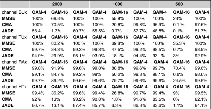
As far as the TUx and RAx channels are concerned, they are associated with less severe multi-path effects: this explains why the JADE algorithm performs well—even better than the CMA for the RAx channel.
2.04.7 Extensions and further readings
2.04.7.1 Case of non-circular sources
Along this paper, the data we considered as circular. This assumption is not crucial for second-order or algebraic methods. However, the presence of a non-circular source in the mixture considerably affects the higher-than-second-order methods. For instance, the fourth-order cumulant ![]() if
if ![]() is the output of a separator, does not have the same expression as when all the sources are circular. It can be even been shown that the separation is not always achieved when two sources are non-circular.
is the output of a separator, does not have the same expression as when all the sources are circular. It can be even been shown that the separation is not always achieved when two sources are non-circular.
The interested reader might find results and references in the following works: [38,58–60].
2.04.7.2 Exploiting the non-stationarity
Cyclo-stationarity is a main statistical feature of the mixture that has long been thought of as a benefit for source separation. For instantaneous BSS using second-order moments, see [61,62]: the idea is that the mixing matrix is constant during the observation, while the second-order statistics of the sources vary. An idea is hence to cut the observation interval in subintervals. Recalling the SOBI approach (see Section 2.04.3.3), the receiver may compute the correlation matrices for the uth interval: ![]() . As the sources are non-stationary, the diagonal matrices
. As the sources are non-stationary, the diagonal matrices ![]() vary with u hence the pencil of matrices to be jointly diagonalized has more elements and the conditions of identifiability are weaker, hence the algorithm is more robust. We refer to the work of Pham [63] for the Maximum Likelihood approach. The reader might be interested by a work of Wang et al. [64].
vary with u hence the pencil of matrices to be jointly diagonalized has more elements and the conditions of identifiability are weaker, hence the algorithm is more robust. We refer to the work of Pham [63] for the Maximum Likelihood approach. The reader might be interested by a work of Wang et al. [64].
In the case of digital communication signals, the cyclo-stationarity is not strong enough in order to consider such approaches: we have pointed out that the power of a source ![]() has very small variations since the cyclo-spectra at the cyclic-frequencies
has very small variations since the cyclo-spectra at the cyclic-frequencies ![]() are numerically small due to the spectral limitation of the shaping functions. On the one hand, the strength of cyclo-stationarity is too weak to be exploited. On the other hand, it cannot be neglected in the computations (for instance in the expression of the fourth-order cumulants).
are numerically small due to the spectral limitation of the shaping functions. On the one hand, the strength of cyclo-stationarity is too weak to be exploited. On the other hand, it cannot be neglected in the computations (for instance in the expression of the fourth-order cumulants).
2.04.7.3 Presence of additive noise
In this paper, we have considered a noise-free model. Many references may be found where the impact of the noise on the BSS methods is analyzed. Among others, we would like to cite the work of Cardoso concerning the performance analysis a class of BSS algorithms who have a the so-called “invariance” feature [35]. Concerning the CMA when noise is present: the reader may have a look at the work of Fijalkow et al. [29] for the use of the CMA as an equalizer algorithm and the proximity of a solution in the presence of noise to a Minimum Mean Square Error (MMSE) equalizer; the case of BSS is analyzed in [25,65] where it is shown that the local minima of the CM cost function are “not far” from MMSE separator. A systematic analysis is provided in Leshem et al. [66] where both the presence of noise and the effect of a finite number of samples are considered.
2.04.8 Conclusion
In this paper, we have given some methods for achieving the BSS in the context of telecommunication. We have focused our attention on contrast functions (joint or deflation-based approaches), and particularly the contrast functions depending on fourth-order statistics of the data. These approaches fit the blind problems evoked in the introduction (spectrum monitoring) since they are associated with convergent and performance algorithms. When the channels involve multi-path effects and no a priori information on the distribution of the delays is available, the deflation-based algorithms such as the CMA or the minimization of the normalized Kurtosis are good candidates for the BSS.
Relevant Theory: Signal Processing Theory and Statistical Signal Processing
See Vol. 1, Chapter 4 Random Signals and Stochastic Processes
See Vol. 3, Chapter 3 Non-stationary Signal Analysis
References
1. Jutten C, Hérault J. Blind separation of sources, Part I—An adaptative algorithm based on neuromimetic architecture. Signal Process. 1991;24:1–10.
2. Comon P. Independent component analysis a new concept? Signal Process. 1994;36(3):287–314 special issue on higher-order statistics.
3. Bingham E, Hyvarinen H. A fast fixed-point algorithm for independent component analysis of complex valued signals. Int J Neural Syst. 2000;10(1):1–8.
4. Cardoso JF, Souloumiac A. Blind beamforming for non gaussian signals. IEE Proc F. 1993;140(6):362–370.
5. Delfosse N, Loubaton P. Adaptative blind separation of independant sources: a deflation approach. Signal Process. 1995;45:59–83.
6. Porat Boaz. A Course in Digital Signal Processing. first ed. Wiley October 1996.
7. Gardner WA. Spectral correlation of modulated signals: Part I—Analog modulations. IEEE Trans Commun. 1987;35:584–594.
8. Napolitano Antonio. Cyclic higher-order statistics: Input/output relations for discrete- and continuous-time MIMO linear almost-periodically time-variant systems. Signal Process. 1995;42(2):147–166.
9. Proakis John. Digital Communications. fourth ed. McGraw-Hill Science/Engineering/Math August 2000.
10. Vaidyanathan PP. Multirate Systems And Filter Banks. first ed. Prentice Hall 1992.
11. Corduneanu C. Almost Periodic Functions. second ed. American Mathematical Society 1989.
12. Gorokhov A, Loubaton P. Subspace-based techniques for blind separation of mixtures with temporally correlated sources. IEEE Trans Circ Syst. 1997;44(9):813–820.
13. Inouye Yujiro, Liu Ruey-Wen. A system-theoretic foundation for blind equalization of an FIR MIMO channel systemchannel system. IEEE Trans Circ Syst.—I. 2002;49(4):425–436.
14. Van Der Veen AJ, Paulraj A. An analytical constant modulus algorithm. IEEE Trans Signal Process. 1996;5(44):1136–1155.
15. Talwar S, Viberg M, Paulraj A. Blind estimation of multiple co-channel digital signals using an antenna array. Signal Process Lett. 1994;1(2):29–31.
16. Talwar S, Viberg M, Paulraj A. Blind separation of synchronous co-channel digital signals using an antenna array—Part I: Algorithms. IEEE Trans Signal Process. 1996;44(5):1184–1197.
17. Agee BG. The least-squares CMA: a new technique for rapid correction of constant modulus signals. In: Proceedings of the ICASSP, Tokyo. 1986;953–956.
18. Gooch RP, Lundell JP. The CM array: an adaptive beamformer for constant modulus signals. In: Proceedings of the ICASSP, Tokyo, Japan. 1986;2523–2526.
19. Belouchrani A, Abed-Meraim K, Cardoso J-F, Moulines E. A blind source separation technique using second-order statistics. IEEE Trans Signal Process. 1997;45(2):434–444.
20. Bunse-Gerstner A, Byers R, Mehrmann V. Numerical methods for simultaneous diagonalization. SIAM J Matrix Anal Appl. 1993;14(4):927–949.
21. Abed-Meraim K, Xiang Y, Manton H, Hua Y. Blind source separation using second-order cyclostationary statistics. IEEE Trans Signal Process. 2001;49(4):694–701.
22. Billingsley Patrick. Probability and Measure. third ed. Wiley-Interscience 1995.
23. Godard DN. Self-recovering equalization and carrier tracking in two-dimensionnal data communication systems. IEEE Trans Commun. 1980;28(11):1867–1875.
24. Sato Y. A method of self-recovering equalization for multilevel amplitude-modulation systems. IEEE Trans Commun. 1975;23(6):679–682.
25. Liu D, Tong L. An analysis of constant modulus algorithm for array signal processing. Signal Process. 1999;73:81–104.
26. Treichler JR, Agee BG. A new approach to multipath correction of constant modulus signals. In: 1983;459–472. IEEE Trans Acoust Speech, Signal Process. vol. 31.
27. Treichler JR, Larimore MG. New processing techniques based on constant modulus adaptive algorithm. IEEE Trans Acoust Speech Signal Process. 1985;33(8):420–431.
28. Regalia PA. On the equivalence between the Godard and Shalvi-Weinstein schemes of blind equalization. Signal Process. 1999;73:185–190.
29. Fijalkow I, Touzni A, Treichler JR. Fractionally spaced equalization using CMA: robustness to channel noise and lack of disparity. IEEE Trans Signal Process. 1998;46(1):227–231.
30. Simon C, Loubaton Ph, Jutten C. Separation of a class of convolutive mixtures: a contrast function approach. Signal Process. 2001;81:883–887.
31. Tugnait JK. Identification and deconvolution of multi-channel non-gaussian processes using higher-order statistics and inverse filter criteria. IEEE Trans Signal Process. 1997;45(3):658–672.
32. Tugnait JK. Adaptive blind separation of convolutive mixtures of independent linear signals. Signal Process. 1999;73:139–152.
33. Marshall Albert W, Olkin Ingram, Arnold Barry. Inequalities: Theory of Majorization and Its Applications. Springer September 2010.
34. Yeredor A. Non-orthogonal joint diagonalization in the least-squares sense with application in blind source separation. IEEE Trans Signal Process. 2002;50(7):1545–1553.
35. Cardoso J-F. On the performance of orthogonal source separation algorithms. In: EUSIPCO, Edinburgh. 1994;776–779.
36. Hyvarinen A. Fast and robust fixed-point algorithms for independent component analysis. IEEE Trans Neural Networks. 1999;10(3):626–634.
37. Mazet L, Loubaton P. Cyclic correlation based symbol rate estimation. In: proc Asilomar Conference on Signals, Systems, and Computers. 1999;1008–1012.
38. Ferréol A, Chevalier P. On the behavior of current second and higher order blind source separation methods for cyclostationary sources. IEEE Trans Signal Process. 2002;48:990 6 (Erratum: 50, N°4) 1712–1725.
39. Jallon P, Chevreuil A. Separation of instantaneous mixtures of cyclostationary sources. Signal Process. 2007;87:2718–2732.
40. Jallon Pierre, Chevreuil Antoine, Loubaton Philippe. Separation of digital communication mixtures with the CMA: case of unknown symbol rates. Signal Process. 2010;2633–2647.
41. Comon Pierre, Jutten Christian. Handbook of Blind Source Separation: Independent Component Analysis and Applications. Academic Press 2010.
42. Van Der Veen AJ, Talwar S, Paulraj A. A subspace approach to blind space-time signal processing for wireless communication systems. IEEE Trans Signal Process. 1997;45(1):173–190.
43. Abed-Meraim K, Loubaton P, Moulines E. A subspace algorithm for certain blind identification problems. IEEE Trans Inform Theory. 1997;43(2):499–511.
44. Swami A, Giannakis GB, Shamsunder S. Multichannel ARMA processes. Trans Signal Process. 1994;42(4):898–913.
45. Gorokhov A, Loubaton Ph. Blind identification of MIMO-FIR systems: a generalized linear prediction approach. Signal Process. 1999;73:104–124.
46. Belouchrani A, Cichocki A. Robust whitening procedure in blind separation context. Electron Lett. 2000;36(24):2050–2051.
47. Brockwell Peter J, Davis Richard A. Time Series: Theory and Methods. second ed. Springer 1991.
48. Comon P. Contrasts for multichannel blind deconvolution. IEEE Signal Process Lett. 1996;3.
49. McWhirter John G, Baxter Paul D, Cooper Tom, Redif Soydan, Foster Joanne. An EVD algorithm for Para-Hermitian polynomial matrices. IEEE Trans Signal Process. 2007;55(5):2158–2169.
50. Comon P, Rota L. Blind separation of independant sources from convolutive mixtures. IEICE Trans Fund Electron Commun Comput Sci. 2003;E86-A(3):542–549.
51. Wang W, Sanei S, Chambers JA. Penalty function-based joint diagonalization approach for convolutive blind separation of non-stationary sources. IEEE Trans Signal Process. 2005;53(5):1654–1669.
52. Hua Yingbo, Tugnait Jitendra K. Blind identifiability of FIR-MIMO systems with colored input using second order statistics. 2000;7(12):348–350.
53. Kawamoto Mitsuru, Inouye Yujiro. Blind deconvolution of MIMO-FIR systems with colored inputs using second-order statistics. IEICE Trans Fund Electron Commun Comput Sci. 2003;E86-A(3):597–604.
54. Kawamoto Mitsuru, Inouye Yujiro. Blind separation of multiple convolved colored signals using second-order statistics. In: Proceedings of the ICA’03, Nara, Japan. 2003.
55. Sabri K, El Badaoui M, Guillet F, Adib A, Aboutajdine D. A frequency domain-based approach for blind MIMO system identification using second-order cyclic statistics. Signal Process. 2009;89(1):77–86.
56. Shalvi O, Weinstein E. New criteria for blind deconvolution of non-minimum phase systems. IEEE Trans Inform Theory. 1990;36:312–321.
57. Loubaton P, Regalia PA. Blind deconvolution of multivariate signals: a deflation approach. In: International Conference on Communications (ICC), Geneva, Switzerland. 1993.
58. Florian E, Chevreuil A, Loubaton P. Blind source separation of convolutive mixtures of non circular linearly modulated signals with unknown baud rates. Signal Process. 2012;92:715–726.
59. Novey M, Adali T. On extending the complex fastica algorithm to non-circular sources. IEEE Trans Signal Process. 2008;56(5):2148–2153.
60. Zhang H, Li L, Li W. Independent vector analysis for convolutive blind non-circular source separation. Signal Process. 2012;92(9):2275–2283.
61. Tsatsanis MK, Kweon C. Source separation using second-order statistics: identifiability conditions and algorithms. In: Asilomar Conference on Signals, Systems and Computers. 1998;1574–1578.
62. Souloumiac A. Blind source detection and separation using second-order nonstationarity. In: ICASSP. 1995;1912–1915.
63. Pham D-T, Cardoso J-F. Blind separation of instantaneous mixtures of nonstationary sources. IEEE Trans Signal Process. 2001;49(9):1837–1848.
64. Wang W, Jafari MG, Sanei S, Chambers JA. Blind separation of convolutive mixtures of cyclo-stationary signals. Int J Adapt Control Signal Process. 2004;18(3):279–298.
65. Tong L, Zeng H, Johnson C. An analysis of constant modulus receivers. IEEE Trans, Signal Process. 1999;47:2990–2999.
66. Leshem A, van der Veen A-J. Blind source separation: the location of local minima in the case of finitely many samples. IEEE Trans Signal Process. 2008;59:4340–4353.