
Signal Processing for Vectored Multichannel VDSL
Itsik Bergel and Amir Leshem, Faculty of Engineering, Bar-Ilan University, Ramat-Gan, Israel
Abstract
Vectored DSL communication systems fall into the category of multiple input multiple output (MIMO) communication systems. As such, they can take advantage of the various MIMO techniques and the vast volume of MIMO research that has been published in recent years. Nevertheless, DSL systems have two unique features that significantly simplify the implementation of MIMO techniques, and hence gave rise to specific DSL research and specific DSL signal processing techniques. These characteristics are the very large coherence time and the diagonal dominance structure of the channel matrix. The diagonal dominant channel matrices have been shown to significantly simplify the interference cancellation between different DSL users. This simplification is crucial to allow MIMO techniques to be applied at the high data rates achievable by modern DSL systems over many lines sharing the same binder. The large coherence time results from the static nature of the communication lines, and also from the continuous activity of DSL links. The very long coherence time allows receivers to obtain very good channel estimates, or alternatively to apply adaptive MIMO techniques that can adapt to the specific channel matrix. In this paper we review the specific DSL research, that has taken advantage of DSL system characteristics and paved the way for very high rate vectored DSL systems.
Keywords
DSL; MIMO; Interference cancellation
2.06.1 Introduction
Digital subscriber line (DSL) is currently the most widespread technique for delivering broadband internet to homes worldwide. By the end of 2010, over 300 million customers were served with DSL, a number representing approximately 60% of global broadband customers. Furthermore, the telephone network infrastructure is still capable of providing the ever increasing demand for larger bandwidth. Data services to home customers began with the use of dialup modems over the public switched telephone network (PSTN). The rates supported by these modems increased from 300 bps in the first commercial modem introduced in 1962 to 56 kbps in the v.92 standardized in 1998. To provide these increasing data rates, more advanced communication and signal processing techniques have been developed. From FSK in the 300 bps mode to a system using advanced precoding, shaping and trellis coding in the v.34 and the newer modems. However, it was clear from the outset that signaling over the 4 kHz voiceband is an unnecessary limitation. In 1988 the UN telecommunication organization CCITT (which was later renamed ITU) defined the Integrated Services Data Networks (ISDN), which support symmetric rates of up to 128 kbps using 256 kHz. At the same time as the development of the ISDN another standard known as the high speed digital subscriber line (HDSL) was developed with the goal of providing operators with a replacement for the expensive T1 (in the US) and E1 (in Europe) lines used to carry 24 or 32 voice channels. The idea was to use improved communication techniques so that the data could be transmitted over regular telephone lines (commonly termed “twisted pairs”) instead of the special lines used previously. HDSL supported rates of up to 2.048 Mbps over two twisted pairs using a 2B1Q baseband modulation (similar to the ISDN modulation) and channel compensation techniques such as a decision feedback equalizer (DFE) and reduced state Viterbi. However transmission was un-coded. A good overview of the HDSL technology is given in [1]. Since transmission over two twisted pairs is costly, a new standard HDSL2 was developed in the US and later extended to the Single Pair High bit rate DSL (SHDSL) by the ITU-T. Concomitantly, an Asymmetric DSL (ADSL) was defined [2] mostly for residential broadband services. ADSL was the first system to use multicarrier modulation, dubbed Discrete Multi-Tone (DMT). In contrast to OFDM, the DMT modulation uses a different bit loading on each carrier and real baseband signaling. Riding on the success of ADSL, the VDSL standard was defined [3]. The major difference between VDSL and ADSL is the larger bandwidth used by the former. This allows for much higher upstream rates, but requires shorter lines. Therefore, the use of the VDSL was delayed until optical network units were deployed in street cabinets and basements. VDSL provided data rates of up to 50 Mbps in the downstream and up to 25 Mbps in the downstream in typical loops of 300 m and above. A good overview of single line DSL technology can be found in books by Starr et al. [4] and Bingham [5].
To understand the ways data rates can be increased beyond VDSL rates, and achieve 100 Mbps symmetric rates over typical twisted pairs, the channel characteristics of the twisted pair channel as well as the crosstalk coupling between twisted pairs in a typical binder of twisted pairs need further explanation. The characterization of the twisted pair channel and its capacity dates back many years. A good example is the paper by Foschini [6] that described the binder using a multiport model. Later, the statistical characteristics of crosstalk at low frequencies using log normal distributions was proposed by Adie and Gibbs [7] and by Lin [8,9]. The models for the average and the 1% worst case were proposed by Werner [10] and refined by Kerpez [11,12]. Kalet and Shamai [13] and Aslanis and Cioffi [14] studied the capacity of single channel DSL systems using the above models. Later Karipidis et al. [15,16] verified these models for frequencies up to 30 MHz, and studied the impact of crosstalk on the capacity of multichannel DSL systems.
These studies make it clear that crosstalk is the limiting factor for increasing the rate of DSL systems. To increase the data rates provided by single line VDSL, the crosstalk between twisted pairs has to be eliminated. This prompted the need for multichannel processing, in which the signals of several modems are jointly processed to overcome the crosstalk between the different twisted pairs. Such systems are often termed “vectored” systems, as the signals of the relevant modems can be ordered in a vector form that enables the use of matrix manipulations and linear algebra tools.
Unlike standard MIMO techniques, crosstalk cancellation in DSL systems can only be done at the network side, where all twisted pairs originate. Lechleider was one of the first to realize that crosstalk cancellation might be an advantage in the context of two pair HDSL systems [17]. Ginis and Cioffi [18] proposed a single sided cancellation in the downstream direction using a multidimensional Tomlinson-Harashima precoder. It was quickly observed that the loss in linear precoding is quite insubstantial, due to the diagonal dominance of the DSL channel [19,20]. In these papers they showed that both upstream and downstream crosstalk cancellation can be done using a linear zero forcing multichannel transmitter (upstream) or receiver (downstream). At the same time, Leshem and Li [21–23] demonstrated that the linear precoder can be simplified even further using an approximated power series expansion. This completely reduced the complexity of the required matrix inversion. Cendrillon et al. [24,25] analyzed the case of partial precoding where only some modems are coordinated.
An alternative adaptive precoder design was proposed by Louvaux and van der Veen [26]. Another simplified version of the adaptive precoder was suggested independently by Louvaux and van der Veen [27] and by Bergel and Leshem [28]. Bergel and Leshem provided a detailed analytic analysis. This analysis showed that there are advantages in not precoding the signals of modems that do not gain much from this precoding, since this can cause significant delay in the convergence of the adaptive precoder. Binyamini et al. [29] generalized this analysis to the case of partial precoding, where similarly to [24] only some of the modems’ signals are precoded.
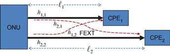
Along with the advances in precoding techniques, initial prototypes were built and an ITU standard G.993.5 was developed that defined the requirements for vectoring VDSL systems. Recently, commercial systems have been developed. These systems use the vectoring capabilities to achieve reliable rates at much larger distances, or to provide much higher data rates for the same line lengths. One of the early prototypes was developed by an Israeli consortium called iSMART, which developed techniques for vectoring. The outcome of this research was the V41 vectoring system developed by ECI Telecom,1 which is depicted in Figure 6.1. A typical vectored VDSL system consists of an ONU, which is typically deployed in a street cabinet or in the basement of high-rise buildings and multiple customer premises equipment units (CPE). The ONU is connected to the operator’s network through a high bandwidth optical link, and contains a multiuser vectored VDSL2 transceiver (V2DSL2) [30], which jointly receives the information from all CPEs and precodes the information transmitted to all CPEs such that all crosstalk between the lines is removed.
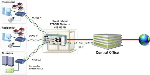
The V41 system can increase the coverage of 50 Mbps service from 400 m to 800 m over 0.4 mm copper twisted pairs. This results in a factor 4 reduction in the ONUs required to provide a universal 50 Mbps service. Similarly, rates of 85 Mbps can be provided at a distance of 400 m.
The purpose of this chapter is to present the mathematical principles behind the current-day massive multi-user systems, serving simultaneously 50–200 customers and canceling interference between all these customers. It is remarkable that similar systems in the wireless domain serve 4–8 customers simultaneously using the same spectrum. The main reason for the success of massive vectoring in the DSL world is that the loss due to zero forcing precoding is marginal because of a channel property called diagonal dominance and the ease of tracking the channels, which are relatively stationary compared to wireless channels.
2.06.2 System model
A typical DSL channel is composed of many users, each connected through a twisted copper wire pair to an Optical Network Unit (ONU), as depicted in Figure 6.2. Many of these twisted pairs are enclosed (at least part of the way) in the same binder. In this work we focus on a group of users that are served through the same binder.
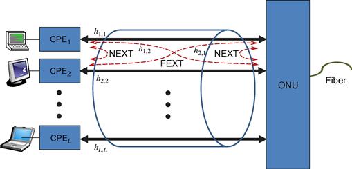
Each user’s modem (termed also customer premises equipment, CPE) aims to transmit data to the network and receive data from the network over its twisted pair. The connection to the network is established through an optical network unit (ONU) which is connected to the network backbone through an optical fiber. The ONU can be located at the telephone switch (also termed central office). However, in recent years, in order to enable higher data rates, the ONU is typically located closer to the users, in street cabinets or even in the users’ building. A shorter distance between the CPE and ONU will result in lower signal attenuation, which can lead to a higher signal to noise ratio (SNR) and higher data rates in the absence of interference. But, as the typical SNR increases, the main limiting factor of DSL systems is inter-user interference.
This inter-user interference results from electromagnetic coupling in the binder, and is divided into two types as shown in Figure 6.2. The crosstalk from signals that originate from the same end as the affected receiver is termed near end crosstalk (NEXT). In VDSL, the impact of NEXT is suppressed by employing frequency-division duplexing (FDD) and transmitters synchronization. The crosstalk from signals that originate from the opposite side of the binder is termed far end crosstalk (FEXT). FEXT is typically the main limiting factor on the performance of DSL systems.
The downstream and upstream of the DSL channel share the same channel, but are rather different in nature. The difference comes from the fact that multichannel processing can be applied only at the ONU. The upstream describes the transmission of data from the CPEs and reception in the ONU. This is a multiple access channel, in which the ONU decodes the data transmitted from multiple CPEs. The downstream describes the transmission of data from the ONU and reception in the CPEs. This is a broadcast channel, in which the ONU transmits data to multiple CPEs while minimizing the interference between the transmitted signals.
Since the upstream and downstream share the same channel, in this section we describe this shared channel. We therefore refer to transmitters and receivers, which will later be translated into CPEs and ONU according to the context. Note that regardless of the actual ONU internal structure, in the following we refer to the ONU as a set of cooperating transmitters/receivers, where each transmitter/receiver is connected to a single twisted pair.
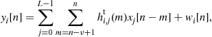
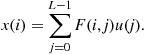
The channel received at the ith receiver is:
 (6.1)
(6.1)
where L is the number of transmitters, ![]() is the sample transmitted by transmitter
is the sample transmitted by transmitter ![]() at time
at time ![]() , and
, and ![]() is the sampled noise. In this model, the sampled noise term can include in addition to thermal noise also interference from various sources such as radio transmissions, neighboring DSL systems and more. Nevertheless, it is generally assumed that the noise samples are independent and identically distributed (i.i.d) Gaussian random variables with zero mean and variance of
is the sampled noise. In this model, the sampled noise term can include in addition to thermal noise also interference from various sources such as radio transmissions, neighboring DSL systems and more. Nevertheless, it is generally assumed that the noise samples are independent and identically distributed (i.i.d) Gaussian random variables with zero mean and variance of ![]() .
.
The impulse response of the channel between the jth transmitter and the ith receiver is denoted by ![]() and
and ![]() is the maximal length of the channel impulse response (also termed the channel memory).2 Note that each receiver is affected by all the transmitters in the system. Thus,
is the maximal length of the channel impulse response (also termed the channel memory).2 Note that each receiver is affected by all the transmitters in the system. Thus, ![]() describes the channels for the direct signals, and
describes the channels for the direct signals, and ![]() for
for ![]() describes the crosstalk channels. Typically, the actual lengths of the various channel impulse responses are different. In the following we take
describes the crosstalk channels. Typically, the actual lengths of the various channel impulse responses are different. In the following we take ![]() to denote the maximal channel memory handled by the system, and assume that all channel impulse responses are zero padded to a length of
to denote the maximal channel memory handled by the system, and assume that all channel impulse responses are zero padded to a length of ![]() .
.
Without loss of generality, in the following we focus on the transmission and reception of symbol number 0, i.e., the block of ![]() input samples,
input samples, ![]() . DSL systems achieve reception that is free of inter symbol interference (ISI) using the discrete Fourier transform (DFT) and a cyclic prefix (CP).
. DSL systems achieve reception that is free of inter symbol interference (ISI) using the discrete Fourier transform (DFT) and a cyclic prefix (CP).
The DFT processing of multiple user signals requires the synchronized reception of all transmissions. Such a synchronization is easily achieved at the downstream, as all transmission originate in the same location. In the upstream, the synchronized reception of all signals transmitted from different CPEs needs more attention. This synchronization is achieved by shifting the transmission time of each CPE according to the delay between the specific CPE and the ONU (using timing feedback from the ONU). This procedure is analogous to the problem of synchronized uplink transmissions in cellular networks. The synchronization timing requirements can be further relaxed using the “Zipper” technique (see [31,32]).
The ![]() samples prior to the transmission of each block are devoted to the CP using:
samples prior to the transmission of each block are devoted to the CP using:
![]() (6.2)
(6.2)
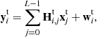
for ![]() . Using (6.2) in (6.1), the vector of output symbols
. Using (6.2) in (6.1), the vector of output symbols ![]()
![]() can be described by:
can be described by:
 (6.3)
(6.3)
where ![]() is the vector of noise samples, and the
is the vector of noise samples, and the ![]() is a circulant channel matrix in which the
is a circulant channel matrix in which the ![]() element is:
element is:
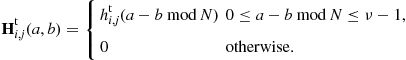 (6.4)
(6.4)
More graphically, the circulant channel matrix has the form:
 (6.5)
(6.5)
In DSL the data processing is performed in the frequency domain using the discrete Fourier transform (DFT). The normalized DFT matrix is given by:
![]() (6.6)
(6.6)
and satisfies ![]() . The transmitted samples of the
. The transmitted samples of the ![]() th user are generated using an inverse DFT (IDFT) operation:
th user are generated using an inverse DFT (IDFT) operation: ![]() . Then, taking the DFT of the output vector, (6.3), results in the frequency domain channel output:
. Then, taking the DFT of the output vector, (6.3), results in the frequency domain channel output:
 (6.7)
(6.7)
where
![]() (6.8)
(6.8)
is the frequency domain channel matrix between transmitter ![]() and receiver
and receiver ![]() , and
, and ![]() is the frequency domain Gaussian noise with zero mean and covariance matrix of
is the frequency domain Gaussian noise with zero mean and covariance matrix of ![]() . Recalling that the time domain channel matrix, (6.4), is a circulant matrix, the frequency domain channel matrix
. Recalling that the time domain channel matrix, (6.4), is a circulant matrix, the frequency domain channel matrix ![]() is a diagonal matrix,3 and hence the received signal matrix is free of ISI.
is a diagonal matrix,3 and hence the received signal matrix is free of ISI.
Although the DSL signal is not degraded by ISI, inspecting the sum in (6.7) one can see that it is highly affected by another type of interference, namely, inter user interference that results from FEXT. To better characterize and resolve the FEXT, it is convenient to restate the input-output relation, grouping all users for each frequency bin separately. Defining ![]() , the output sample at the
, the output sample at the ![]() th frequency bin for all users can be described by:
th frequency bin for all users can be described by:
![]() (6.9)
(6.9)
where ![]() is the vector of samples transmitted by all users,
is the vector of samples transmitted by all users, ![]()
![]() is the vector of noise measured by all users and the combined channel matrix is given by:
is the vector of noise measured by all users and the combined channel matrix is given by:
![]() (6.10)
(6.10)
In most cases, the processing and analysis of DSL signals is performed for a single frequency bin at a time. Thus, the relation described by Eq. (6.9) is very useful. In many cases we will even drop the frequency bin indices (f ) where the specific frequency bin number is not crucial.
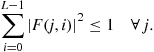
The power constraint is also stated in the frequency domain in the form of a spectrum power mask. In the following we assume that all users follow the same spectrum mask, and the power constraint is given by:
![]() (6.11)
(6.11)
2.06.2.1 Channel matrix structure
As the FEXT results from electromagnetic coupling and not from a direct wire connection, in most frequencies the FEXT is significantly smaller from the direct signal. Thus, it has been noted [19] that upstream VDSL channel matrices are column-wise diagonally dominant (CWDD), while downstream matrices are row-wise diagonally dominant (RWDD). This diagonal dominance channel matrix structure is one of the main features that distinguish DSL systems from other MIMO systems. Hence, most DSL specific research has used this feature in some way or another.
For simplicity we will first describe the RWDD structure of the downstream channel and then comment on the upstream channel. Basically, in a RWDD matrix, the diagonal element dominates all other elements in the row. The weakest definition states that a matrix is weakly RWDD if
![]() (6.12)
(6.12)
for ![]() . One can also quantify how much is the matrix RWDD using:
. One can also quantify how much is the matrix RWDD using:
![]() (6.13)
(6.13)
A matrix is weakly RWDD if ![]() , and as
, and as ![]() decreases the matrix is said to be “more” RWDD.
decreases the matrix is said to be “more” RWDD.
An alternative measure compares the diagonal element to the sum of the absolute values of the elements in the rest of the row:
![]() (6.14)
(6.14)
A matrix that satisfies ![]() is said to be strongly RWDD.
is said to be strongly RWDD.
If all pairs in the binder have the same length, the magnitude of the diagonal elements in the matrix is nearly identical, and the matrix can be termed simply diagonally dominant. The differentiation between RWDD and CWDD is important mostly in mixed length scenarios. Figure 6.3 depicts a 2-user mixed length downstream scenario with a short link of length ![]() and a long link of length
and a long link of length ![]() . Note that the FEXT is only generated in the joint part (of length
. Note that the FEXT is only generated in the joint part (of length ![]() ). Thus, the FEXT into the short link is equivalent to the FEXT in the case of equal link binder, and it is significantly smaller than the direct link signal. For the longer link, the FEXT contribution can be split into a cascade of two systems: in the first system there is a FEXT contribution into the
). Thus, the FEXT into the short link is equivalent to the FEXT in the case of equal link binder, and it is significantly smaller than the direct link signal. For the longer link, the FEXT contribution can be split into a cascade of two systems: in the first system there is a FEXT contribution into the ![]() initial segment of the link, and in the second system this FEXT is further attenuated by a link of length
initial segment of the link, and in the second system this FEXT is further attenuated by a link of length ![]() . Hence its mean response is [10]:
. Hence its mean response is [10]:
![]() (6.15)
(6.15)
where ![]() is the typical loop insertion loss at length
is the typical loop insertion loss at length ![]() and frequency f and
and frequency f and ![]() is a constant that depends on the type of cable. Note that from the equal length case we already concluded that
is a constant that depends on the type of cable. Note that from the equal length case we already concluded that ![]() . Recalling that
. Recalling that
![]() (6.16)
(6.16)
the cascade of the two LTI systems shows that
![]() (6.17)
(6.17)
From (6.17) we can conclude that an even more accurate representation of the channel matrix structure is given by [22]:
![]() (6.18)
(6.18)
where the matrix ![]() has zeros on its diagonal and all its elements are (significantly) smaller than one. This type of definition turns out to be important for the convergence analysis of adaptive precoders. The corresponding measure is:
has zeros on its diagonal and all its elements are (significantly) smaller than one. This type of definition turns out to be important for the convergence analysis of adaptive precoders. The corresponding measure is:
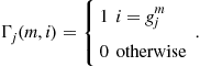
 (6.19)
Note that although the sum in the first maximization in (6.19) is taken over rows and the sum in the second maximization is taken over columns, both are measures of RWDD. This is because in both cases each matrix element, ![]() , is divided by the diagonal element in its own row,
, is divided by the diagonal element in its own row, ![]() . Thus the
. Thus the ![]() serves as another indication that no element in the matrix is significant compared to the diagonal element in its row.
serves as another indication that no element in the matrix is significant compared to the diagonal element in its row.
As for the upstream, one only needs to observe that due to the channel reciprocity, the upstream channel matrix at each frequency is the transpose of the upstream channel matrix at the same frequency. DSL systems work in FDD mode and hence no frequency is used simultaneously for both upstream and downstream. However, for channel characterization purposes the channel reciprocity holds, and we can simply apply the above definitions ((6.13), (6.14) and (6.19)) to the transposed channel matrix. Thus, we define:
![]() (6.20)
(6.20)
![]() (6.21)
(6.21)
and
 (6.22)
A matrix is weakly CWDD if ![]() , and strongly CWDD if
, and strongly CWDD if ![]() . The channel decomposition of (6.18) is replaced from the upstream with: [22]:
. The channel decomposition of (6.18) is replaced from the upstream with: [22]:
![]() (6.23)
(6.23)
where the matrix ![]() has the same characteristics as the matrix
has the same characteristics as the matrix ![]() , i.e., it has a zero on its diagonal and all its elements are (significantly) smaller than one.
, i.e., it has a zero on its diagonal and all its elements are (significantly) smaller than one.
To demonstrate the diagonal dominance of the channel matrices, Figure 6.4 depicts the values of ![]() and
and ![]() as a function of frequency for binder lengths of 150–300 m. It is clear that, at both lengths, the channel matrices are strongly diagonal dominant for practically all frequencies. In this plot we do not show
as a function of frequency for binder lengths of 150–300 m. It is clear that, at both lengths, the channel matrices are strongly diagonal dominant for practically all frequencies. In this plot we do not show ![]() , as it was nearly identical to
, as it was nearly identical to ![]() for all frequencies at both binder links.Note on figures: All the numerical results in this paper rely on channel measurements carried out by France Telecom at different lengths over a binder with 28 twisted pairs.4 All simulations presented here were carried out under the assumption that the whole bandwidth of the VDSL system is completely dedicated to the downstream or completely dedicated to the upstream. The transmission SNR is set to
for all frequencies at both binder links.Note on figures: All the numerical results in this paper rely on channel measurements carried out by France Telecom at different lengths over a binder with 28 twisted pairs.4 All simulations presented here were carried out under the assumption that the whole bandwidth of the VDSL system is completely dedicated to the downstream or completely dedicated to the upstream. The transmission SNR is set to ![]() (corresponding to the typical values of
(corresponding to the typical values of ![]() and
and ![]() , where
, where ![]() is the symbol length).
is the symbol length).

2.06.3 Downstream transmission
2.06.3.1 Nonlinear precoding
In the downstream (or in its more general term: the broadcast channel) the receiving modems are located in different customer premises and cannot cooperate to achieve FEXT cancellation. On the other hand, the transmitting modems are co-located at the ONU, and hence FEXT cancellation is feasible using joint signal processing of the transmitted symbols.
Ginis and Cioffi [18] considered the use of a QR decomposition followed by a Tomlinson-Harashima like modulo operation [33,34]. Considering the LQ decomposition of the channel matrix we can write:
![]() (6.24)
(6.24)
where ![]() is a unitary matrix and
is a unitary matrix and ![]() is a lower triangular matrix. An even more convenient representation is the QR decomposition of the conjugate transpose of the channel matrix, given by
is a lower triangular matrix. An even more convenient representation is the QR decomposition of the conjugate transpose of the channel matrix, given by ![]() where
where ![]() is an upper triangular matrix.
is an upper triangular matrix.
Let ![]() denote the modulated symbols that need to be transmitted in the
denote the modulated symbols that need to be transmitted in the ![]() th frequency bin by all users. In the following we consistently assume that the modulated symbols of all users in the same subcarrier are iid random variables (which is reasonable given our assumption that all users comply with the same spectral mask). We further assume that
th frequency bin by all users. In the following we consistently assume that the modulated symbols of all users in the same subcarrier are iid random variables (which is reasonable given our assumption that all users comply with the same spectral mask). We further assume that ![]() and
and ![]() .
.
The modulated symbols are first precoded to reduce interference due to the matrix ![]() :
:
 (6.25)
where the modulo operation is defined by:
![]() (6.26)
(6.26)
the index ![]() gives the constellation size for user
gives the constellation size for user ![]() , i.e.,
, i.e., ![]() is the number of possible modulation values for the real part of
is the number of possible modulation values for the real part of ![]() multiplied by the distance between modulation points,
multiplied by the distance between modulation points, ![]() is the number of possible modulation values for the imaginary part of
is the number of possible modulation values for the imaginary part of ![]() multiplied by the distance between modulation points. The operation
multiplied by the distance between modulation points. The operation ![]() is a modulo type operation that returns values in the range
is a modulo type operation that returns values in the range ![]() , i.e.,
, i.e., ![]() .
.
Figure 6.5 illustrates this precoding with a modulo operation for the case of QPSK modulation. The possible modulation values are depicted by circles. The allowed transmission range is depicted by the middle square, and its modulo equivalents are depicted by dashed squares. The transmitter wishes to transmit the top right modulation value ![]() . The solid arrow represents the subtraction of interference from previous users, and hence, the square mark represents the value to be transmitted in order to achieve full interference cancellation without the modulo operation. The dashed arrow represents the modulo operation, and the final resulting precoded value,
. The solid arrow represents the subtraction of interference from previous users, and hence, the square mark represents the value to be transmitted in order to achieve full interference cancellation without the modulo operation. The dashed arrow represents the modulo operation, and the final resulting precoded value, ![]() , is represented by the x-mark.
, is represented by the x-mark.

In order to achieve interference-free reception, the symbols, ![]() , still need to be rotated using the matrix
, still need to be rotated using the matrix ![]() . This rotation is given by:
. This rotation is given by:
![]() (6.27)
(6.27)
It is easy to verify that without the modulo operation, this scheme already achieves complete FEXT cancellation. The role of the modulo operation is to reduce the power increase due to the FEXT cancellation (just as in the classic Tomlinson-Harashima setting [33,34]).
To reciprocate the modulo operation, each receiver performs the modulo operation:
![]() (6.28)
(6.28)
To verify the FEXT cancellation, we substitute (6.9), (6.24), (6.25), and (6.27) in (6.28) and get:
 (6.29)
where the last line results from ![]() . It is further shown in [18] that the noise increase as well as the power increase are negligible in DSL systems, hence resulting in a near optimal FEXT free communication scheme.
. It is further shown in [18] that the noise increase as well as the power increase are negligible in DSL systems, hence resulting in a near optimal FEXT free communication scheme.
The above method can be interpreted as a suboptimal implementation of the zero-forcing “dirty-paper” precoding scheme proposed in [35] and studied in [36]. An improvement of the scheme was proposed in [37], where Tomlinson-Harashima precoding was replaced by more efficient trellis precoding schemes. The broadcast channel has been further studied in many works, mostly in the context of wireless MIMO systems. However, for DSL systems, most of the focus has shifted to linear precoders that combine very good performance and lower implementation complexity.
2.06.3.2 Linear precoding
2.06.3.2.1 The zero forcing precoder
Linear precoders have often been considered for low complexity interference cancellation over broadcast channels. A linear precoder transmits a signal which is a linear combination of the modulated data symbols. Denoting the precoding matrix by ![]() , the transmitted vector for all users is given by:
, the transmitted vector for all users is given by:
![]() (6.30)
(6.30)
The linear precoder must satisfy the system power constraint. Assuming that all users have the same power constraint in each frequency (same spectral mask) and that the modulated data symbols ![]() satisfies the power constraint, the constraint on the precoder is given by:
satisfies the power constraint, the constraint on the precoder is given by:
 (6.31)
Linear precoders attracted considerable attention in DSL systems mostly following the work of Cendrillon et al. [38]. In that work, the authors showed that the zero forcing (ZF) precoder achieves near optimal performance in most DSL channels. Cendrillon et al. adopted the ZF linear precoder given by:
![]() (6.32)
(6.32)
where ![]() is the diagonal matrix with the same diagonal elements as
is the diagonal matrix with the same diagonal elements as ![]() and
and ![]() is a constant chosen to satisfy the power constraint (6.31). (In that work they termed this precoder the diagonalizing precoder, to distinguish it from the more trivial ZF precoder:
is a constant chosen to satisfy the power constraint (6.31). (In that work they termed this precoder the diagonalizing precoder, to distinguish it from the more trivial ZF precoder: ![]() .) Obviously, substituting (6.32) and (6.30) in (6.9) results in FEXT free reception:
.) Obviously, substituting (6.32) and (6.30) in (6.9) results in FEXT free reception:
![]() (6.33)
(6.33)
and the achievable data rate by user ![]() in any specific subcarrier is given by:
in any specific subcarrier is given by:
![]() (6.34)
(6.34)
where ![]() is the gap between the used precoder performance and the actual capacity (commonly termed the Shannon gap [39]), and
is the gap between the used precoder performance and the actual capacity (commonly termed the Shannon gap [39]), and ![]() is the symbol rate.
is the symbol rate.
The main question is how large can ![]() be. In their work Cendrillon et al. [38] showed that
be. In their work Cendrillon et al. [38] showed that ![]() can typically be set very close to 1, and hence the ZF precoder achieves near optimal performance. The key to this near optimality is the structure of the DSL channel matrix, and in particular the row-wise diagonally dominant (RWDD) channel matrix. To prove this, they presented an upper bound on the capacity and a lower bound on the achievable data rates using the ZF linear precoder. Here we present the simpler (but generally tighter) bounds of Bergel and Leshem [40], which rely on the strong diagonal dominance measures. The upper bound is described by the following theorem.
can typically be set very close to 1, and hence the ZF precoder achieves near optimal performance. The key to this near optimality is the structure of the DSL channel matrix, and in particular the row-wise diagonally dominant (RWDD) channel matrix. To prove this, they presented an upper bound on the capacity and a lower bound on the achievable data rates using the ZF linear precoder. Here we present the simpler (but generally tighter) bounds of Bergel and Leshem [40], which rely on the strong diagonal dominance measures. The upper bound is described by the following theorem.
Theorem 1
The data rate achievable by user![]() in any specific subcarrier of the downstream of DSL systems is upper bounded by:
in any specific subcarrier of the downstream of DSL systems is upper bounded by:
![]() (6.35)
(6.35)
Proof
Considering only the ![]() th receiver. Taking into account the channel structure, (6.9), and the power constraint on the precoder, (6.31), the maximal signal power for this user is achieved using a precoder in which only the
th receiver. Taking into account the channel structure, (6.9), and the power constraint on the precoder, (6.31), the maximal signal power for this user is achieved using a precoder in which only the ![]() th column is non-zero, and the absolute value of all elements in this column is 1. Using such a precoder, the maximal signal power for the
th column is non-zero, and the absolute value of all elements in this column is 1. Using such a precoder, the maximal signal power for the ![]() th user is:
th user is: ![]() . Calculating the achievable user rate, and maximizing over all users results in (6.35), and completes the proof of the theorem.
. Calculating the achievable user rate, and maximizing over all users results in (6.35), and completes the proof of the theorem.
On the other side we have:
Theorem 2
[40]
The data rate achievable by user![]() in any specific subcarrier when the ONU applies a ZF precoder is lower bounded by:
in any specific subcarrier when the ONU applies a ZF precoder is lower bounded by:
![]() (6.36)
(6.36)
where
![]() (6.37)
(6.37)
Figure 6.6 depicts the achievable performance using a ZF precoder and compares it to the upper and lower bounds. In this figure, as well as in all numerical rates evaluation in what follows, we assume a 0 dB Shannon gap, i.e., ![]() . Note that the bounds are tight for low frequencies. For such frequencies
. Note that the bounds are tight for low frequencies. For such frequencies ![]() is very small, and comparing (6.35) and (6.36) the bound tightness for small enough
is very small, and comparing (6.35) and (6.36) the bound tightness for small enough ![]() is obvious. For higher frequencies the lower bound becomes useless when
is obvious. For higher frequencies the lower bound becomes useless when ![]() . Yet, the actual ZF performance is still very close to the upper bound for all frequencies. For reference, the figure also depicts the achievable rates without precoding, and the achievable rates in the single user case, i.e., when only a single twisted pair in the binder is used. It shows that ZF performance nearly matches the single user performance and is significantly higher than the no precoding scheme. However, although the single user performance seems as worthy target, it is important to note that this curve is not a performance bound. This is because we cannot rule out the possibility that the inter-user connections will be used to increase user capacity. In particular, the upper bound corresponds to the case where all the inter-user connections for one of the users are used to increase this user’s capacity. Thus, the importance of the upper bound is in showing that even in the most optimistic case, the achievable rate cannot exceed the ZF rates by more than 10%.
. Yet, the actual ZF performance is still very close to the upper bound for all frequencies. For reference, the figure also depicts the achievable rates without precoding, and the achievable rates in the single user case, i.e., when only a single twisted pair in the binder is used. It shows that ZF performance nearly matches the single user performance and is significantly higher than the no precoding scheme. However, although the single user performance seems as worthy target, it is important to note that this curve is not a performance bound. This is because we cannot rule out the possibility that the inter-user connections will be used to increase user capacity. In particular, the upper bound corresponds to the case where all the inter-user connections for one of the users are used to increase this user’s capacity. Thus, the importance of the upper bound is in showing that even in the most optimistic case, the achievable rate cannot exceed the ZF rates by more than 10%.
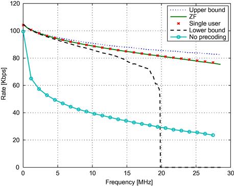
Figure 6.6 Average achievable user rate over a single subcarrier and bounds, as a function of the subcarrier frequency, at a 150 m binder.
Figure 6.7 shows that the Cendrillon et al. [38] bounds were ahead of their time. The figure depicts the actual achievable rate in the case that all of the VDSL bandwidth is dedicated to the downstream vs. the distance between the ONU and the CPEs. The figure also presents the upper bound of Theorem 3 and the lower bound of Theorem 2. It is clear that the bounds are tighter and the achievable data rate is higher for shorter link distances. In recent years, as the optical fibers deployment has expanded, the lengths of VDSL links have continually decreased. Hence, although the bounds presented by Cendrillon et al. were not tight for the typical link length at the time, nowadays, and certainly in the future, the typical link length is much shorter, and the bounds can be considered tight.
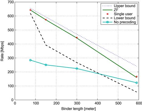
Nevertheless, it should be pointed out that the final conclusions of Cendrillon et al. [38] hold for all practical link distances. Comparing the achievable data rates of the ZF precoder to the upper bound shows that the precoder is indeed close to optimal. Furthermore, the performance of the ZF precoder is nearly identical to the more reasonable target of the single user performance (i.e., a system with a single user, transmitting over only one twisted pair).
2.06.3.2.2 Reduced complexity ZF precoding
The use of linear precoders reduces the transmitter implementation complexity, and does not require any modification of the CPE (the downstream receivers). But as DSL technology achieves ever higher data rates, the implementation complexity of linear receivers is still too high. The implementation complexity is composed of the computation of the precoding matrix, and the computation of the precoded signals using the precoding matrix.
To reduce the complexity of the first part, Leshem and Li [22] suggested computing the precoder matrix using a first or second order approximation of the channel matrix. As stated above, the ![]() power normalization constant in (6.32) is very close to 1. Neglecting this power normalization constant, the ZF precoder is given by:
power normalization constant in (6.32) is very close to 1. Neglecting this power normalization constant, the ZF precoder is given by:
![]() (6.38)
(6.38)
Using the notation of (6.18) the ZF precoder can be rewritten as:
![]() (6.39)
(6.39)
As shown in [28], if ![]() , then the maximal singular value of
, then the maximal singular value of ![]() is smaller than one, and hence the ZF precoder, (6.39), can be represented by a converging Taylor expansion:
is smaller than one, and hence the ZF precoder, (6.39), can be represented by a converging Taylor expansion:
![]() (6.40)
(6.40)
Hence, they suggested using a first or second order Taylor approximation of (6.40), which eliminates the need for matrix inversion.
The first order approximation is given by:
![]() (6.41)
(6.41)
The complexity reduction is significant in that the matrix inverse operation in (6.38) is replaced by the inverse of a diagonal matrix, which requires only ![]() single element inversions. For the cases in which the first order approximation is not accurate enough, Leshem and Li suggested using the second order approximation, given by:
single element inversions. For the cases in which the first order approximation is not accurate enough, Leshem and Li suggested using the second order approximation, given by:
![]() (6.42)
(6.42)
See [22] for a detailed analysis of this implementation approach and the complexity reduction factor.
They also provided a lower bound on the performance of their proposed precoders. Interestingly, their bounds require only a form of weak RWDD, i.e., the bounds hold even in cases where the Taylor expansion in (6.40) might not converge. For example, for the first order ZF precoder they give the following bound:
Theorem 3
[22]
If the channel matrix is weekly RWDD, and satisfies![]() , then the data rate achievable by user
, then the data rate achievable by user![]() in any specific subcarrier of the downstream of a DSL system that applies the first order precoder given in (6.41) is lower bounded by:
in any specific subcarrier of the downstream of a DSL system that applies the first order precoder given in (6.41) is lower bounded by:
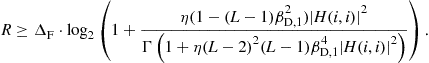 (6.43)
Figure 6.8 shows the performance of the approximated precoders over real channel measurements. As can be seen, the first order approximation is good when the FEXT is low (in particular at low frequencies). For higher frequencies, the first order approximation precoder still achieves reasonable precoding at a link distance of 300 m (a capacity loss of around 10%). As link distances get shorter, the SNR increases and the FEXT cancellation of the first order approximation is not sufficient, as can be seen for the 75 m binder in the figure. On the other hand, the second order approximation precoder achieves near optimal performance in all the tested scenarios.
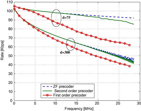
Figure 6.8 Average achievable user rate over a single subcarrier as a function of the subcarrier frequency, for the ZF precoder, and its first and second order approximation. The figure shows results for a 75 m binder and for a 300 m binder.
However, the computational complexity of the matrix inversion is not the only problem. With 4000 symbols per second, and thousands of subcarriers, even the application of the precoder (i.e., the multiplication ![]() ) requires too many computations. This implementation complexity has been researched from two points of view. First, the number of bits per sample needs to be considered.
) requires too many computations. This implementation complexity has been researched from two points of view. First, the number of bits per sample needs to be considered.
2.06.3.2.3 Quantization of word length for ZF precoding
Sayag et al. [41] studied the effect of word length on the performance of ZF precoders. Their main theorem formulates the capacity loss in a system that uses ![]() bits for the quantization of the real part and
bits for the quantization of the real part and ![]() bits for the quantization of the imaginary part of the precoding matrix. Their main theorem is:
bits for the quantization of the imaginary part of the precoding matrix. Their main theorem is:
Theorem 4
If the number of quantization bits of the ZF precoder satisfies![]() , then the transmission rate loss of the
, then the transmission rate loss of the![]() th user at any specific subcarrier due to quantization is upper bounded by:
th user at any specific subcarrier due to quantization is upper bounded by:
![]() (6.44)
(6.44)
In their work they further studied the rate loss using the Werner channel model [10], and show, for example, that a quantization of 14 bits for the real part and 14 bits for the imaginary part is sufficient to guarantee a rate loss of no more than 1% for links of 300 m or more. Note that shorter links experience higher signal levels, and hence the FEXT cancellation requirements are stricter (thus requiring more quantization bits).
2.06.3.2.4 Partial ZF precoding
Another way to reduce the complexity of FEXT cancellation is to cancel only some of the interference sources. Writing explicitly the computation of each transmitted symbol, from (6.30) we have:
 (6.45)
Thus, every zero element in the precoder matrix, ![]() , saves one multiplication. Cendrillon et al. [25] studied the performance of ZF DSL precoders with various constraints on the number of non-zero elements in
, saves one multiplication. Cendrillon et al. [25] studied the performance of ZF DSL precoders with various constraints on the number of non-zero elements in ![]() .
.
Given the set of interference sources to be canceled for each user, the evaluation of the optimal precoder is not trivial. Cendrillon et al. suggested an adjustment of the ZF criterion for this case, by reducing the number of constraints. If the total number of non-zero elements in the precoding matrix ![]() is
is ![]() , one can solve a system of
, one can solve a system of ![]() linear equations, i.e., force
linear equations, i.e., force ![]() zeros in the resulting effective channel,
zeros in the resulting effective channel, ![]() . Cendrillon et al. showed how to solve this ZF problem when the zero elements of
. Cendrillon et al. showed how to solve this ZF problem when the zero elements of ![]() are in the same locations as the zero elements in the precoding matrix,
are in the same locations as the zero elements in the precoding matrix, ![]() . The description given here is slightly more general than the original, to include also the equations needed for partial adaptive precoding presented in Section 2.06.3.3.
. The description given here is slightly more general than the original, to include also the equations needed for partial adaptive precoding presented in Section 2.06.3.3.
Let ![]() be the set of receivers that need to cancel the FEXT originating from user
be the set of receivers that need to cancel the FEXT originating from user ![]() . Denote the set size by
. Denote the set size by ![]() .5 We define the ZF partial precoder as:
.5 We define the ZF partial precoder as:
![]() (6.46)
(6.46)
where the matrix ![]() satisfies
satisfies ![]() for any
for any ![]() . The elements with non-zero values in
. The elements with non-zero values in ![]() are constructed according to the generalization of the ZF principle, which completely cancels the FEXT generated by the
are constructed according to the generalization of the ZF principle, which completely cancels the FEXT generated by the ![]() th user to all users
th user to all users ![]() . To simplify the precoder analysis we define the (
. To simplify the precoder analysis we define the (![]() ) selection matrices,
) selection matrices, ![]() :
:
 (6.47)
Applying the partial ZF criterion, the ![]() th column of the precoder is constructed to satisfy:
th column of the precoder is constructed to satisfy:
![]() (6.48)
(6.48)
where ![]() is the
is the ![]() th column of the matrix
th column of the matrix ![]() . Note that
. Note that ![]() has zeros in the rows that do not belong to the set
has zeros in the rows that do not belong to the set ![]() ; thus, the non-zero elements of
; thus, the non-zero elements of ![]() are given by
are given by ![]() , and:
, and:
![]() (6.49)
(6.49)
Substituting (6.46) and (6.49), in (6.48) we have:
![]() (6.50)
(6.50)
and the non-zero elements of ![]() are given by:
are given by:
![]() (6.51)
(6.51)
Note that ![]() is a non singular matrix formed by the elements of the channel matrix that are located in the rows and columns that belong to
is a non singular matrix formed by the elements of the channel matrix that are located in the rows and columns that belong to ![]() (i.e., by
(i.e., by ![]() ). Partial precoder results with residual FEXT whose powers (for all users) are given by the diagonal of:
). Partial precoder results with residual FEXT whose powers (for all users) are given by the diagonal of:
 (6.52)
However, the utilization of a partial precoder requires the transmitter to first obtain a good enough channel estimation, and then apply a good enough selection algorithm. Cendrillon et al. [25] considered several user selection algorithms. They tested a binder with 8 users in which users at 900 m could increase their rate by 72% using complete FEXT cancellation. They showed that by proper user selection, a system can achieve 41% of this rate increase with only 20% of the implementation complexity. They also considered a FEXT cancellation over only part of the DMT subcarriers, and showed that a scheme that performs both user and tone selection can perform even better and achieve 77% of the rate increase with 20% of the implementation complexity. (Note however for shorter link lengths that FEXT is more dominant and the gains with the same implementation complexity will be smaller). Figure 6.11 below also depicts the performance of a partial precoder for a 28 user binder over a length of 300 m. Note that ![]() represents the number of multiplications per precoding operation, averaged over all subcarriers. Again a significant part of the rate gain can be achieved with a relatively small part of the complexity. Vangorp et al. [42] extended this work, and presented a low complexity algorithm for optimal resource allocation given limited complexity for the partial FEXT cancellation.
represents the number of multiplications per precoding operation, averaged over all subcarriers. Again a significant part of the rate gain can be achieved with a relatively small part of the complexity. Vangorp et al. [42] extended this work, and presented a low complexity algorithm for optimal resource allocation given limited complexity for the partial FEXT cancellation.
Uplink partial FEXT cancellation was also considered in the same framework [24]. We will not describe this here in more detail, since the analysis and results are quite similar. It should be noted that for the upstream Pandey et al. [43] also considered a partial MMSE receiver. But as demonstrated in Section 2.06.4.1, the MMSE receiver does not gain much in most common scenarios.
2.06.3.3 Adaptive precoding
The use of low complexity linear precoders made FEXT cancellation feasible in high rate DSL systems. However, recall that in the downstream the transmitter at the ONU cannot directly measure the channel matrix. Hence, the calculation of the precoding matrix must rely on feedback from the receivers. Two main types of feedback have been considered: channel estimation feedback and signal error feedback.
Channel estimation feedback is based on the transmission of orthogonal (synchronized) pilot symbols from all transmitters simultaneously, and an estimation of a row of the channel matrix by each receiver. This estimated row is then transmitted (through the upstream) back to the transmitter, which uses it to construct the full channel matrix ![]() and to calculate the precoding matrix
and to calculate the precoding matrix ![]() . This approach mostly uses standard (and not DSL specific) techniques, and hence has mostly been discussed in implementation oriented publications.
. This approach mostly uses standard (and not DSL specific) techniques, and hence has mostly been discussed in implementation oriented publications.
Signal error feedback is a more DSL specific method, and is based on the feedback of a quantized version of the error signal measured by each receiver. The error signal measured by the ![]() th receiver is:
th receiver is:
![]() (6.53)
(6.53)
The ONU collects all error signals feedback into a vector:
![]() (6.54)
(6.54)
This error signal vector can be used by the transmitter to adapt a precoder that attempts to minimize the error signal energy.
However, because the error signal is measured by the receiver, it needs to be quantized and sent back to the receiver. We assume hereafter that the error signal is first normalized and then quantized. Each receiver normalizes its error signal by dividing it with the direct channel gain, ![]() . Thus, the quantized error signal
. Thus, the quantized error signal ![]() can be written as:
can be written as:
![]() (6.55)
(6.55)
and ![]() is the quantization error. Note that
is the quantization error. Note that ![]() can be statistically dependent on
can be statistically dependent on ![]() .
.
Adaptive precoding for DSL was first suggested by Louveaux and van der Veen [26]. They considered an adaptive precoder designed to minimize the norm ![]() . Taking the derivative with respect to the precoding matrix, using the instantaneous correlation matrix and taking some approximations, they suggested using the update equation:
. Taking the derivative with respect to the precoding matrix, using the instantaneous correlation matrix and taking some approximations, they suggested using the update equation:
![]() (6.56)
(6.56)
where the subscript indicates the time (i.e., ![]() , and
, and ![]() denotes the value at time
denotes the value at time ![]() of the precoding matrix the received symbol and modulated data, respectively),
of the precoding matrix the received symbol and modulated data, respectively), ![]() is the precoder update constant, and
is the precoder update constant, and ![]() denotes the operation of zeroing all diagonal elements of a matrix. They also considered the use of a quantized version of the received signal, but gave no details. This adaptive precoder was studied only by simulations.
denotes the operation of zeroing all diagonal elements of a matrix. They also considered the use of a quantized version of the received signal, but gave no details. This adaptive precoder was studied only by simulations.
A simpler version of an adaptive precoder was proposed independently by Louveaux and van der Veen [27] and by Bergel and Leshem [28]. Their suggested precoder update is given by6:
![]() (6.57)
(6.57)
This adaptive precoder has much lower implementation complexity than (6.56), as it does not include multiplication by the inverse matrix. This precoder is also simpler in terms of analysis. In [28] Bergel and Leshem considered the simplified case of rich enough quantization, such that the quantization error, ![]() is statistically independent on the error signal
is statistically independent on the error signal ![]() . For this simplified case they provided both convergence bounds and a steady state error analysis. The convergence is guaranteed by the following theorem:
. For this simplified case they provided both convergence bounds and a steady state error analysis. The convergence is guaranteed by the following theorem:
Theorem 5
[28]
A sufficient condition for the precoder given by(6.57)to converge is that:
![]() (6.58)
(6.58)
where![]() i.e.,
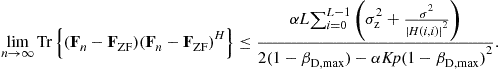
i.e.,![]() . If(6.58)is satisfied, then after sufficiently long convergence time, the Frobenius norm of the difference between the zero forcing precoder
. If(6.58)is satisfied, then after sufficiently long convergence time, the Frobenius norm of the difference between the zero forcing precoder![]() and the adaptive precoder is upper bounded by:
and the adaptive precoder is upper bounded by:
 (6.59)
where![]() is the variance of the quantization noise
is the variance of the quantization noise![]() .
.
As can be seen in Figure 6.4 the strong RWDD condition in the theorem (![]() ) is satisfied practically for all frequencies for link distances of up to 300 m. Thus, the precoder is very robust, and can converge in all channels. As
) is satisfied practically for all frequencies for link distances of up to 300 m. Thus, the precoder is very robust, and can converge in all channels. As ![]() is typically not known in advance, a practical approach would be to take its maximal value when choosing the update constant, and use
is typically not known in advance, a practical approach would be to take its maximal value when choosing the update constant, and use ![]() . In such case, (6.59) simplifies to:
. In such case, (6.59) simplifies to:
 (6.60)
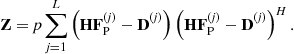
The convergence bound is important to guarantee the converge of the precoder. However, once the precoder has converged to a steady state, (6.59) does not provide a convenient performance measure, as it relates to the precoder error and not to the final performance. In the same work they also provide a more convenient steady state approximation. For large enough ![]() (so that the precoder reaches steady state), the covariance matrix of the error signal is approximated by:
(so that the precoder reaches steady state), the covariance matrix of the error signal is approximated by:
![]() (6.61)
(6.61)
where ![]() is the variance of the quantization noise. The covariance matrix in (6.61) is composed of two terms. The first is the error increase due to the use of the iterative precoder (note that the error signal covariance matrix with no FEXT is I). This error increase is negligible if
is the variance of the quantization noise. The covariance matrix in (6.61) is composed of two terms. The first is the error increase due to the use of the iterative precoder (note that the error signal covariance matrix with no FEXT is I). This error increase is negligible if ![]() . The second term is due to the quantization error, and does not depend on the noise power.
. The second term is due to the quantization error, and does not depend on the noise power.
Nevertheless, the simplifying assumption of rich quantization [28] is impractical, because such a quantization would cause a high feedback rate, and overload the upstream. Louveaux and van der Veen [44] presented an approximate analysis for the case of phase feedback only, under the assumption that the signal of each modem can be analyzed independently (which holds for very low ![]() ). In a recent work, Binyamini and Bergel [45] analyzed the same precoder with low rate quantization. In particular they considered a low bit rate dithered [46] uniform quantization only of the phase of the error signal. This work showed that the precoder will converge for any update constant,
). In a recent work, Binyamini and Bergel [45] analyzed the same precoder with low rate quantization. In particular they considered a low bit rate dithered [46] uniform quantization only of the phase of the error signal. This work showed that the precoder will converge for any update constant, ![]() , and for any quantization level (even 1 bit per sample) as long as the channel is strongly RWDD and
, and for any quantization level (even 1 bit per sample) as long as the channel is strongly RWDD and ![]() .
.
Their quantization scheme uses a sequence of pseudo random phase variables, ![]() , which are designed to behave as iid random variabled uniformly distributed over
, which are designed to behave as iid random variabled uniformly distributed over ![]() (in the what follows we assume that this is their actual distribution). This sequence is known in advance both at the transmitter and at all receivers. The error signal of the
(in the what follows we assume that this is their actual distribution). This sequence is known in advance both at the transmitter and at all receivers. The error signal of the ![]() th user at time
th user at time ![]() , is first rotated by multiplying it with
, is first rotated by multiplying it with ![]() , and then quantized to one of the values
, and then quantized to one of the values ![]() , where
, where ![]() , and
, and ![]() is the number of quantization values. At the transmitter, the actual quantization value is obtained by multiplying the received quantization level by
is the number of quantization values. At the transmitter, the actual quantization value is obtained by multiplying the received quantization level by ![]() . Thus, the quantized error signal can be written as:
. Thus, the quantized error signal can be written as:
 (6.62)
and ![]() is the phase quantization error. Note that the dithering operation ensures that the phase quantization error is an iid sequence, and each element is uniformly distributed over
is the phase quantization error. Note that the dithering operation ensures that the phase quantization error is an iid sequence, and each element is uniformly distributed over ![]() . In [45] the authors show that the dithering has a negligible effect on system performance, and is required mostly for analysis purposes, due to the convenient distribution of the quantization error. The convergence of a precoder that employs a dithered phase quantization scheme is guaranteed by:
. In [45] the authors show that the dithering has a negligible effect on system performance, and is required mostly for analysis purposes, due to the convenient distribution of the quantization error. The convergence of a precoder that employs a dithered phase quantization scheme is guaranteed by:
Theorem 6
[45]
Considering an adaptive precoder of the form of(6.57)which uses dithered phase quantization as described in(6.62). If![]() , the precoder converges, and after a sufficiently long convergence time, the averaged in time expectation on the absolute error measured by the
, the precoder converges, and after a sufficiently long convergence time, the averaged in time expectation on the absolute error measured by the![]() th receiver is upper bounded by:
th receiver is upper bounded by:
 (6.63)
The theorem shows that the error signal is bounded by a noise increase of ![]() plus an additional term which is linear with the precoder update constant,
plus an additional term which is linear with the precoder update constant, ![]() . Thus, it is feasible to approach FEXT free performance by a choosing small enough precoder update, up to the noise increase term.
. Thus, it is feasible to approach FEXT free performance by a choosing small enough precoder update, up to the noise increase term.
Naturally such low rate quantization results in lower performance than the rich quantization in Theorem 5 (i.e., slower convergence and/or higher steady state errors). Nevertheless, unlike Theorem 5, the phase quantization scheme in Theorem 6 achieves convergence for every value of the update constant. Note however that the bound (6.63) is not very tight. The authors observed that a better approximation of the actual error signal magnitude is obtained by substituting ![]() in (6.63) instead of the actual value of
in (6.63) instead of the actual value of ![]() .
.
Figure 6.9 shows the (averaged over all users) normalized error signal magnitude of two adaptive precoders vs. the time (in symbols), over the subcarrier at a frequency of 5.78 MHz. The lower curve shows the magnitude of the error signal, divided by ![]() , in the precoder of (6.57) with no quantization and with
, in the precoder of (6.57) with no quantization and with ![]() (about half the maximal allowed value). The doted curve with stars shows the steady state approximation in (6.61) for the no quantization case (i.e.,
(about half the maximal allowed value). The doted curve with stars shows the steady state approximation in (6.61) for the no quantization case (i.e., ![]() ). The higher curve depicts the magnitude of the error signal, divided by
). The higher curve depicts the magnitude of the error signal, divided by ![]() when the adaptive precoder employs the low rate quantization of Theorem 6 with
when the adaptive precoder employs the low rate quantization of Theorem 6 with ![]() (1-bit feedback) and
(1-bit feedback) and ![]() (note that the measured user gain at this frequency is
(note that the measured user gain at this frequency is ![]() ). As can be seen, the precoder converges at about the same time as the no quantization precoder, but with much higher error signal magnitude. The dashed line shows the cumulative averaged in time error signal divided by
). As can be seen, the precoder converges at about the same time as the no quantization precoder, but with much higher error signal magnitude. The dashed line shows the cumulative averaged in time error signal divided by ![]() , and the dotted line with triangles depicts the steady state bound of (6.63). The dotted line with circles shows the steady state approximation (calculated by substituting
, and the dotted line with triangles depicts the steady state bound of (6.63). The dotted line with circles shows the steady state approximation (calculated by substituting ![]() in (6.63)). As can be seen, the precoders converge reasonably fast, and the suggested approximations are quite good.
in (6.63)). As can be seen, the precoders converge reasonably fast, and the suggested approximations are quite good.

To further demonstrate the accuracy of the suggested steady state error magnitude approximations, Figure 6.10 shows the average steady state error magnitude and compares it to the approximations of (6.61) and (6.63) vs. the normalized precoder update constant. (Note that in order to match the approximation expressions, the average is taken over the absolute value of the error signal magnitude for the low rate precoder, while for the non quantized precoder the average is taken over the square magnitude). The normalized precoder update constant is given by ![]() for the no quantization case, and by
for the no quantization case, and by ![]() for the low rate quantization precoder. One can see that both approximations are quite good. In particular, the low rate quantization precoder approximation holds even for very high values of
for the low rate quantization precoder. One can see that both approximations are quite good. In particular, the low rate quantization precoder approximation holds even for very high values of ![]() . This demonstrates the claim of Theorem 6 that the precoder converges for every value of
. This demonstrates the claim of Theorem 6 that the precoder converges for every value of ![]() . Note however that very high values of
. Note however that very high values of ![]() are not desirable, as they can cause even a FEXT increase compared to the original no precoding scheme.
are not desirable, as they can cause even a FEXT increase compared to the original no precoding scheme.

Figure 6.10 Steady state error signal magnitude vs. normalized precoder update constant. The normalized precoder update constant is given by ![]() for the no quantization case (marked by stars), and by
for the no quantization case (marked by stars), and by ![]() for the low rate quantization precoder (marked by circles).
for the low rate quantization precoder (marked by circles).
The situation is slightly more complicated in mixed length scenarios, where the different pairs in the binder reach destinations at different distances. From (6.59) it can be seen that the precoder convergence is dominated by the channel gain of the user with the longest (weakest) link. On the other hand, in many cases, these weak users are noise limited and not FEXT limited, and hence FEXT cancellation is not useful for them. For this reason, it was suggested in [28] not to implement FEXT cancellation for such users, based on an SNR threshold test. (Note that the FEXT from these users to other users is still canceled.) Such an approach was shown to significantly shorten the convergence times in mixed length scenarios.
Binyamini et al. [29] observed that partial FEXT cancellation is also desirable to reduce implementation complexity. In this work the partial FEXT cancellation described above (in which some users do not employ FEXT cancellation at all) is termed partial FEXT cancellation of type I. They also define a partial FEXT cancellation of type II, where (for some users) only the FEXT from a subgroup of the users is canceled. This precoder takes advantage of the implementation complexity gain described by Cendrillon et al. [25] and in Section 2.06.3.2.4.
They suggested a simple adaption of the precoder in (6.57), which does not update the precoder at the non-canceled terms. The mathematical formulation (as well as the analysis) of this type of precoder is more complicated, as its update equation cannot be described in a matrix form. Instead, the precoder update for the ![]() th column is given by:
th column is given by:
![]() (6.64)
(6.64)
where the matrix ![]() describes the selected users for FEXT cancellation as described in Section 2.06.3.2.4. Note that the set of
describes the selected users for FEXT cancellation as described in Section 2.06.3.2.4. Note that the set of ![]() update Eq. (6.64),
update Eq. (6.64), ![]() , are actually coupled, because the error signal at the
, are actually coupled, because the error signal at the ![]() th symbol depends on all the columns of the precoding matrix that were updated in the
th symbol depends on all the columns of the precoding matrix that were updated in the ![]() th symbol.
th symbol.
Although the analysis is more complicated, Binyamini et al. [29] showed that it complies with the same sufficient convergence condition as in the full update precoder (Theorem 5). More specifically:
Theorem 7
[29]
Assuming that the quantization noise is statistically independent of the error signal, a sufficient condition for the partial precoder given by(6.64)to converge is that:
![]() (6.65)
(6.65)
If(6.65)is satisfied, then after sufficiently long convergence time, the Frobenius norm of the difference between the precoder![]() and the non-adaptive partial precoder
and the non-adaptive partial precoder![]() that satisfies(6.48) and (6.49) is upper bounded by:
that satisfies(6.48) and (6.49) is upper bounded by:
 (6.66)
where![]() is the variance of the quantization noise
is the variance of the quantization noise![]() and
and![]() is the residual FEXT of the non-adaptive partial FEXT precoder, i.e., the
is the residual FEXT of the non-adaptive partial FEXT precoder, i.e., the![]() th element on the diagonal of the covariance residual FEXT covariance matrix,
th element on the diagonal of the covariance residual FEXT covariance matrix,![]() given in(6.52).
given in(6.52).
In the same work, they also provide a steady state approximation which is demonstrated to be quite accurate. This approximation is given by:
 (6.67)
where ![]() is the total number of elements used in the partial adaptive precoder. Note that the sum over
is the total number of elements used in the partial adaptive precoder. Note that the sum over ![]() is the power of the noise plus residual FEXT in the non-adaptive partial precoder of Section 2.06.3.2.4. Thus, the term
is the power of the noise plus residual FEXT in the non-adaptive partial precoder of Section 2.06.3.2.4. Thus, the term ![]() represents the increase in the error signal power due to the adaptive precoding. The second term in the right hand side of (6.67) represents the effect of the error signal quantization noise,
represents the increase in the error signal power due to the adaptive precoding. The second term in the right hand side of (6.67) represents the effect of the error signal quantization noise, ![]() .
.
The performance of the partial adaptive precoder is depicted in Figure 6.11, with a comparison to the non adaptive partial precoder described in Section 2.06.3.2.4. The figure depicts the average user rates (when all the bandwidth is allocated to the downstream) using partial precoding as a function of time, for various complexity levels. The case of ![]() corresponds to full FEXT cancellation (i.e., in this case all the precoding matrix is updated). The performance in this case are identical to the performance described above. In the two other cases
corresponds to full FEXT cancellation (i.e., in this case all the precoding matrix is updated). The performance in this case are identical to the performance described above. In the two other cases ![]() represents the number of non-zero elements in the precoding matrix, averaged over all sub-carriers. It is clear that the adaptive partial precoder converges quite fast, and achieves rates close to those of the non-adaptive precoder. Note also that the difference between the adaptive and non-adaptive precoders is smaller for smaller values of
represents the number of non-zero elements in the precoding matrix, averaged over all sub-carriers. It is clear that the adaptive partial precoder converges quite fast, and achieves rates close to those of the non-adaptive precoder. Note also that the difference between the adaptive and non-adaptive precoders is smaller for smaller values of ![]() . This behavior is consistent with the approximation in (6.67), which shows that the additional FEXT due to the adaptive precoding is linear with
. This behavior is consistent with the approximation in (6.67), which shows that the additional FEXT due to the adaptive precoding is linear with ![]() .
.
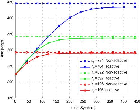
Figure 6.11 Average achievable user rate over the whole bandwidth at a 300 m 28 user binder, using a adaptive and non-adaptive partial precoders.
It is worth noting that the selection of the important terms for FEXT cancellation has not been studied so far in the context of adaptive precoding. This is an open issue because adaptive precoding systems do not employ channel estimation, and only use the error signal feedback to adapt the precoder. Thus, such systems are required to select the important FEXT terms based on this error signal feedback. This can be done for example by testing long term correlations between the error signals and the transmitted symbols. Alternatively, one can try to use the precoder adaption as a learning mechanism, adapt the precoder for some test elements and then use the resulting precoder to decide on the significance of each element. Further research is required to define such methods and characterize their performance.
An alternative to the adaptive precoding scheme using error signal feedback is adaptive precoding using SNR measurement feedback, as presented by Whiting et al. [47]. The major advantage of this approach is that it requires only SNR feedback reports, which are inherent to all VDSL modems. Thus, adaptive FEXT cancellation can be applied without any change in the CPE. But, SNR reports have no phase information, and hence a more complex algorithm is required to learn the correct direction for precoder adaptation. The updated algorithm is composed of several stages in which the various lines are perturbed in various directions. Then the received SNR reports are compiled into an adaption of the precoder, and the process starts over again. Whiting et al. [47] provided convergence bounds and analytic expressions for the convergence time and expected performance. Comparing to the adaptive precoding using error signal described above, one should keep in mind that SNR feedback adaptive precoding does not require any change in the CPE. On the other hand, its main disadvantage is its convergence time, which is several orders of magnitude slower (hundreds of symbols, i.e., less than a second using error signal feedback compared to minutes and even hours using SNR feedback).
2.06.4 Upstream transmission
2.06.4.1 Linear receiver
In the upstream, the receiving modems are colocated at the ONU. This allows for joint reception of the signals transmitted on the different twisted pairs. As was the case for the downstream, upstream performance has also been shown to be nearly optimized with a ZF receiver [48]. Using
![]() (6.68)
(6.68)
and recalling that the upstream channel matrix is CWDD, Cendrillon et al. [48] presented bounds that guarantee that ZF precoder performance is very close to the maximal achievable performance. Their upper bound is given by:
Theorem 8
[48]
The data rate achievable by user![]() in any specific subcarrier of the upstream of DSL systems is upper bounded by:
in any specific subcarrier of the upstream of DSL systems is upper bounded by:
![]() (6.69)
(6.69)
For the lower bound, we give here the bound from [40], which is slightly better than the original bound in [48]:
Theorem 9
[40]
The data rate achievable by user![]() in any specific subcarrier of the upstream of DSL systems when the ONU applies a ZF receiver is lower bounded by:
in any specific subcarrier of the upstream of DSL systems when the ONU applies a ZF receiver is lower bounded by:
![]() (6.70)
(6.70)
In some cases, the system is subject to interference from alien sources. This interference can be highly correlated between the different twisted pairs in the binder. Unlike the downstream, in the upstream the receiver can take advantage of this correlation and reduce the effect of alien interference. The ZF receiver does not take advantage of this correlation, and hence can suffer a dramatic decrease in capacity, as seen for example in Figure 6.12. To better visualize why the ZF receiver can be far from optimal in this case, one can consider a noise whitening approach:
![]() (6.71)
(6.71)
where ![]() is the covariance matrix of
is the covariance matrix of ![]() , which includes both noise and interference. The resulting channel model is quite similar to the initial model in that the resulting noise is white (
, which includes both noise and interference. The resulting channel model is quite similar to the initial model in that the resulting noise is white (![]() ). However, Chen et al. [49,50] observed that in some cases, the resulting effective channel matrix,
). However, Chen et al. [49,50] observed that in some cases, the resulting effective channel matrix, ![]() , is no longer diagonal dominant. Thus, Theorem 9 does not help, and ZF performance can be far from optimal.7
, is no longer diagonal dominant. Thus, Theorem 9 does not help, and ZF performance can be far from optimal.7
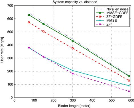
Figure 6.12 Average achievable user rate over the whole bandwidth in the upstream vs. binder length, for various receiver structures.
Pandey et al. [43] suggested that a MMSE linear receiver can gain from the alien noise correlation. They showed that for an 1200 m link in the presence of strong alien noise an MMSE receiver can achieve rates 5 times better than the rates achievable by ZF, and more than half of the actual capacity. However, for shorter link lengths, the signal power becomes more significant. Hence the MMSE receiver focuses on FEXT cancellation, and its performance is very close to the performance of the ZF receiver (see Figure 6.12).
2.06.4.2 Decision feedback equalizer
For cases in which the linear processing discussed above is too far from optimal, Chen et al. [50] proposed using a ZF generalized decision feedback equalizer (GDFE). The authors demonstrate that the ZF-GDFE is a simplified version of the MMSE-GDFE, which was shown to achieve optimal capacity in the Gaussian multiple access channel [51]. In the following we do not describe the MMSE-GDFE, as this general technique was developed mostly for wireless channels and has no particular characteristics in DSL systems.
In the ZF-GDFE scheme, the receiver applies a QR decomposition of the channel ![]() of (6.71):
of (6.71):
![]() (6.72)
(6.72)
where ![]() is a unitary matrix and
is a unitary matrix and ![]() is an upper triangular matrix. Rotating the input by:
is an upper triangular matrix. Rotating the input by:
![]() (6.73)
(6.73)
results in a simpler structure, which is convenient for GDFE. Due to the upper triangular structure of ![]() , the last user in the model of (6.73) receives the transmitted signal with no interference. This user is decoded first.8 Then, the effect of the decoded user is subtracted from the received signal, and the second user can be decoded with no interference. This scheme continues, until the effect of users 1 through
, the last user in the model of (6.73) receives the transmitted signal with no interference. This user is decoded first.8 Then, the effect of the decoded user is subtracted from the received signal, and the second user can be decoded with no interference. This scheme continues, until the effect of users 1 through ![]() is subtracted, and user number 0 is decoded with no interference.
is subtracted, and user number 0 is decoded with no interference.
Note that in this description user number 0 has the highest priority, as the effect of all users is subtracted before its decoding. In order to optimize system performance, user priorities must be controlled. This is done by reordering the users before the detection. In addition, one can control the power allocation between the different users. Such an optimization is described in [50] (see also [52] for such an optimization for the MMSE-GDFE receiver).
On the other hand Leshem and Zehavi [53] noted that in DSL systems, the spectral mask power constraint is more dominant. Thus, the optimization with respect to the transmission powers is much simpler than in the problem considered by [50]. When the spectral mask power constraint is dominant, the optimal power allocation simply uses the maximal allowed power for each user at each subcarrier.
As for the user priorities and ordering, it turns out that in most cases there exists a trivial ordering that results in near optimal performance. For example, in the simulation of Figure 6.12, the ZF-GDFE receiver does not optimize user priorities, and selects user ordering in a random manner. The figure depicts the performance of several receiver types over various link lengths. The simulation includes 28 users and alien noise which is 30 dB stronger than the white noise. Without the alien noise, all receivers achieve nearly the same performance which is very close to channel capacity. In the presence of alien noise, the ZF receiver performs very poorly. The MMSE receiver performs somewhat better, but this advantage only holds for the longer link distances. As explained above, for short links the performance of the MMSE receiver is nearly identical to the performance of the ZF receiver. On the other hand, the ZF-GDFE receiver performs quite well, and can achieve ![]() of the channel capacity. Note that the channel capacity (achievable using the MMSE-GDFE receiver) is only slightly affected by the presence of the alien noise.
of the channel capacity. Note that the channel capacity (achievable using the MMSE-GDFE receiver) is only slightly affected by the presence of the alien noise.
It should be noted that complete FEXT cancellation may not always be feasible in near future practical systems. One factor is the complexity of MMSE-GDFE receivers that may prevent complete FEXT cancellation in the presence of alien noise. Another factor is the large amount of deployed CPEs that do not support vectoring. Thus, in the coming years we expect to see many systems that are partially vectored and partially non-vectored. In such cases it is important to combine FEXT cancellation techniques with dynamic spectrum management (DSM) techniques (see for example [54,55]).
2.06.5 Conclusion
This chapter discussed the properties of the DSL multi-access and broadcast channels. It provided the basic system and channel models and presented the main solutions for both upstream and downstream. It is clear that a massive deployment of G.993.5 will take place in the near future. These systems perform multi-user MIMO-DMT transmission and reception using an order of 4000 tones and providing rates up to 100 Mbps. This massive vectoring is extremely important for reducing the need for fiber to the home deployment, and will enable aggregate rates larger than 5 Gbps for 64 users over distances of up to 800 m. Vectored DSL systems provide an excellent illustration of the fact that fitting signal processing and communication techniques to the specific properties of the channel at hand results in excellent performance at moderate computational cost.
Relevant Theory: Signal Processing Theory
See Vol. 1, Chapter 9 Discrete Multi-Scale Transforms in Signal Processing
References
1. Lechleider J. Coordinated transmission for two-pair digital subscriber lines. IEEE J Sel Areas Commun. 1991;9(6):920–930.
2. Symmetric Digital Subscriber Line (ADSL) Transceivers, ITU-T Recommendation G.992.1, SERIES G: Transmission Systems and Media, Digital Systems and, Networks, 1999.
3. ITU-T Recommendation G.993.1-2004: Very High Speed Digital Subscriber Line. SERIES G: Transmission Systems and Media, Digital Systems and Networks, October 2004.
4. Starr T, Cioffi JM, Silverman P. Understanding Digital Subscribe Line Technology. Upper Saddle River, NJ: Prence-Hall; 1999.
5. Bingham JAC. ADSL, VDSL, and Multicarrier Modulation. John Wiley & Sons Inc. 2000.
6. Foschini G. Crosstalk in outside plant cable systems. Bell Syst Tech J. 1971;50(7):2421–2450.
7. Addie R, Gibbs A. The covariance of near end crosstalk and its application to pcm system engineering in multipair cable. IEEE Trans Commun. 1979;27(2):469–477.
8. Lin S. Statistical behaviour of multipair crosstalk. Bell Syst Tech J. 1980;59(6):955–974.
9. Lin S. Statistical behaviour of multipair crosstalk with dominant components. Bell Syst Tech J. 1980;59.
10. Werner J. The HDSL environment. IEEE J Sel Areas Commun. 1991;9(6):785–800.
11. Kerpez K. Near-end crosstalk is almost gaussian. IEEE Trans Commun. 1993;41(5):670–672.
12. K. Kerpez, Models for the number of next disturbers and next loss, Tech. Rep., 1999, t1E1.4/99-471 (Online). Available: <ftp://ftp.t1.org/pub/t1e1/e1.4/DIR99/9e144710.pdf>.
13. Kalet I, Shamai (Shitz) S. On the capacity of a twisted pair: Gaussian model. IEEE Trans Commun. 1990;38(3):379–383.
14. Aslanis J, Cioffi J. Achievable information rates on digital subscriber loops: limiting information rates with crosstalk. IEEE Trans Commun. 1992;40(2):361–372.
15. Karipidis E, Sidiropoulos N, Leshem A, Li Y. Experimental evaluation of capacity statistics for short VDSL loops. IEEE Trans Commun. 2005;53(7):1119–1122.
16. Karipidis E, Sidiropoulos N, Leshem A, Li Y, Tarafi R, Ouzzif M. Crosstalk models for short VDSL2 lines from measured 30MHz data. EURASIP J Appl Signal Process. 2006;2006 90–90.
17. Lechleider J. Coordinated transmission for two-pair digital subscriber lines. IEEE J Sel Areas Commun. 1991;9(6):920–930.
18. Ginis G, Cioffi J. Vectored transmission for digital subscriber line systems. IEEE J Sel Areas Commun. 2002;20(5):1085–1104.
19. Cendrillon R, Moonen M, Verlinden J, Bostoen T, Ginis G. Improved linear crosstalk precompensation for DSL. In: IEEE International Conference on Acoustics, Speech and Signal Processing, Montreal, Canada. May 2004;4.
20. Cendrillon R, Moonen M, Bostoen T, Ginis G. The linear zero-forcing crosstalk canceller is near-optimal in DSL channels. In: IEEE Global Communications Conference, TX, Dallas. 2004;5.
21. Leshem A, Li Y. A low complexity coordinated fext cancellation for VDSL. In: Proceedings of IEEE ICECS 2004. December 2004;338–341.
22. Leshem A, Li Y. A low complexity linear precoding technique for next generation VDSL downstream transmission over copper. IEEE Trans Signal Process. 2007;55(11):5527–5534.
23. Li Y, Leshem A. A lower bound on the performance of simplified linear precoding for vectored DSL. Int J Pure Appl Math. 2008;43.
24. Cendrillon R, Moonen M, Ginis G, Van Acker K, Bostoen T, Vandaele P. Partial crosstalk cancellation for upstream VDSL. EURASIP J Appl Signal Process. 2004;2004:1520–1535.
25. Cendrillon R, Ginis G, Moonen M, Van Acker K. Partial crosstalk precompensation in downstream VDSL. Signal Process. 2004;84(11):2005–2019.
26. Louveaux J, van der Veen A. Adaptive DSL crosstalk precancellation design using low-rate feedback from end users. IEEE Signal Process Lett. 2006;13(11):665–668.
27. Louveaux J, van der Veen A-J. Adaptive Precoding for Downstream Crosstalk Precancelation in DSL Systems Using Sign-Error Feedback. IEEE Trans Signal Process. 2010;58(6):3173–3179.
28. Bergel I, Leshem A. Convergence Analysis of Downstream VDSL Adaptive Multichannel Partial FEXT Cancellation. IEEE Trans Commun. 2010;58(10):3021–3027.
29. Binyamini I, Bergel I, Leshem A. Arbitrary partial FEXT cancellation in adaptive precoding for multichannel downstream VDSL. IEEE Trans Signal Process. 2012;60(11):5754–5763.
30. ITU-T Recommendation G.993.5-2010, Self-FEXT Cancellation (Vectoring), 2010.
31. Sjöberg F, Isaksson M, Nilsson R, Ödling P, Wilson S, Börjesson P. Zipper: a duplex method for VDSL based on DMT. IEEE Trans Commun. 1999;47(8):1245–1252.
32. Mestdagh D, Isaksson M, Ödling P. Zipper VDSL: a solution for robust duplex communication over telephone lines. IEEE Commun Mag. 2000;38(5):90–96.
33. Tomlinson M. New automatic equaliser employing modulo arithmetic. Electron Lett. 1971;7(5):138–139.
34. Harashima H, Miyakawa H. Matched-transmission technique for channels with intersymbol interference. IEEE Trans Commun. 1972;20(4):774–780.
35. Caire G, Shamai S. On achievable rates in a multi-antenna broadcast downlink. In: Proc 38th Annu Allerton Conf Communication, Control and, Computing. 2000;1188–1193.
36. Caire G, Shamai S. On the achievable throughput of a multiantenna gaussian broadcast channel. IEEE Trans Inform Theory. 2003;49(7):1691–1706.
37. Yu W, Cioffi J. Trellis precoding for the broadcast channel. IEEE Global Telecommunications Conference, 2001, GLOBECOM’01. 2001;2:1344–1348.
38. Cendrillon R, Ginis G, Van den Bogaert E, Moonen M. A near-optimal linear crosstalk precoder for downstream VDSL. IEEE Trans Commun. 2007;55(5):860–863.
39. Cioffi J, Dudevoir G, Eyuboglu M, Forney Jr G. MMSE decision-feedback equalizers and coding II Coding results. IEEE Trans Commun. 1995;43(10):2595–2604.
40. Bergel I, Leshem A. The performance of zero forcing DSL systems. IEEE Signal Process Lett. 2013;20(5):527–530.
41. Sayag E, Leshem A, Sidiropouios ND. Finite word length effects on transmission rate in zero forcing linear precoding for multichannel DSL. IEEE Trans Signal Process. 2009;57(4):1469–1482.
42. Vangorp J, Tsiaflakis P, Moonen M, Verlinden J, Ysebaert G. Dual decomposition approach to partial crosstalk cancelation in a multiuser DMT-xDSL environment. EURASIP J Adv Signal Process. 2007;2007:1–11.
43. Pandey P, Moonen M, Deneire L. MMSE-based partial crosstalk cancellation for upstream VDSL. In: IEEE International Conference on Communications (ICC). 2010.
44. Louveaux J, van der Veen A. Adaptive precoding for downstream crosstalk precancelation in DSL systems using sign-error feedback. IEEE Trans Signal Process. 2010;58(6):3173–3179.
45. Binyamini, Bergel I. Adaptive precoder using sign error feedback for FEXT cancellation in multichannel downstream VDSL. IEEE Trans Signal Process. 2013;61(9):2383–2393.
46. Gray M, Stockham TG. Dithered quantizers. IEEE Trans Inform Theory. 1993;39.
47. Whiting P, Kramer G, Nuzman C, Ashikhmin A, van Wijngaarden A, Živković M. Analysis of inverse crosstalk channel estimation using SNR feedback. IEEE Trans Signal Process. 2011;59:1102–1115.
48. Cendrillon R, Ginis G, Van den Bogaert E, Moonen M. A near-optimal linear crosstalk canceler for upstream VDSL. IEEE Trans Signal Process. 2006;54(8):3136–3146.
49. Chen C, Seong K, Zhang R, Cioffi J. Optimized transmission for upstream vectored DSL systems using zero-forcing generalized decision-feedback equalizers. In: Proc IEEE Globecom. 2006.
50. Chen C, Seong K, Zhang R, Cioffi J. Optimized resource allocation for upstream vectored DSL systems with zero-forcing generalized decision feedback equalizer. IEEE J Sel Top Signal Process. 2007;1(4):686–699.
51. Varanasi M, Guess T. Optimum decision feedback multiuser equalization with successive decoding achieves the total capacity of the gaussian multiple-access channel. Conference Record of the 31st Asilomar Conference on Signals, Systems and Computers. 1997;2:1405–1409.
52. Tsiaflakis P, Vangorp J, Verlinden J, Moonen M. Multiple access channel optimal spectrum balancing for upstream DSL transmission. IEEE Commun Lett. 2007;11 398–300.
53. Leshem A, Zehavi E. Rate control for PSD limited multiple access systems through linear programming. In: IEEE International Conference on Acoustics, Speech and Signal Processing (ICASSP). 2011;3220–3223.
54. Chan V, Yu W. Joint multiuser detection and optimal spectrum balancing for digital subscriber lines. EURASIP J Appl Signal Process. 2006;2006:1–13.
55. A. Chowdhery, J. Cioffi, Dynamic spectrum management for upstream mixtures of vectored and non-vectored DSL, in: IEEE Global, Telecommunications Conference (GLOBECOM).
1We thank Ido Shargil from ECI Telecom for providing the information on the v41 platform.
2We use the notation ![]() to indicate time domain quantities. In the following we will also use the notations
to indicate time domain quantities. In the following we will also use the notations ![]() and
and ![]() to indicate frequency domain quantities.
to indicate frequency domain quantities.
3Recalling that the eigenvalue decomposition of a circulant matrix contains the DFT and IDFT matrices, and a diagonal frequency domain channel matrix.
4The authors thank M. Ouzzif, R. Tarafi, H. Marriott, and F. Gauthier of France Telecom R&D, who conducted the VDSL channel measurements under the auspices of the U-BROAD project.
5Note that we allow the set ![]() to be empty. On the other hand, Cendrillon et al. [25] required
to be empty. On the other hand, Cendrillon et al. [25] required ![]() to always include at least the element
to always include at least the element ![]() . As can be seen from (6.46), setting
. As can be seen from (6.46), setting ![]() does not increase the implementation complexity. Thus,
does not increase the implementation complexity. Thus, ![]() is required only in the context of adaptive precoding.
is required only in the context of adaptive precoding.
6The version by Louveaux and van der Veen only takes the non-diagonal elements of the update matrix. This version is not described here as its analysis is more complicated.
7Note that in most cases, vectored VDSL systems coordinate all pairs in the binder. In such cases, the alien noise is usually negligible.
8Decoding can mean the decoding of the complete code word for this user. But due to complexity constraints, a more typical approach just takes hard decisions on the symbol value.