
Multi-Channel SAR for Ground Moving Target Indication
Stefan V. Baumgartner and Gerhard Krieger, German Aerospace Center (DLR), Microwaves and Radar Institute, Oberpfaffenhofen, Germany, [email protected], [email protected]
Abstract
Modern multi-channel air- and spaceborne synthetic aperture radar (SAR) sensors allow for a variety of applications, independent of sunlight illumination and weather conditions. One application is ground moving target indication (GMTI) with the aim to detect moving targets on ground and to estimate their positions, velocities and moving directions. Although originated in the military field, nowadays GMTI also has gained relevance for civilian road traffic monitoring to ensure the mobility and to increase the safety of the road users. The actual chapter provides a comprehensive tutorial for GMTI with SAR systems. The effects on SAR imagery caused by moving targets are addressed in detail. Additionally, the basic moving target detection and parameter estimation techniques used in state-of-the-art multi-channel algorithms are treated. Finally an outlook to future trends is given.
Keywords
Ground moving target indication (GMTI); Along-track interferometry (ATI); Space-time adaptive processing (STAP); Synthetic aperture radar (SAR); Multi-channel SAR
Nomenclature
a acceleration magnitude of the target (![]() )
)
![]() complex coefficient containing free-space attenuation, backscattering coefficient, and two-way antenna pattern weighting
complex coefficient containing free-space attenuation, backscattering coefficient, and two-way antenna pattern weighting
![]() bandwidth of the clutter Doppler spectrum (Hz)
bandwidth of the clutter Doppler spectrum (Hz)
![]() bandwidth of the transmitted pulse (Hz)
bandwidth of the transmitted pulse (Hz)
![]() speed of light in vacuum (m/s)
speed of light in vacuum (m/s)
![]() physical along-track antenna separation (m)
physical along-track antenna separation (m)
![]() effective along-track phase center separation (m)
effective along-track phase center separation (m)
![]() Doppler or azimuth frequency (Hz)
Doppler or azimuth frequency (Hz)
![]() probability density function of cluster-plus-noise
probability density function of cluster-plus-noise
![]() Doppler shift of the moving target signal (Hz)
Doppler shift of the moving target signal (Hz)
![]() Doppler shift of the stationary target signal (Hz)
Doppler shift of the stationary target signal (Hz)
![]() probability density function of target-plus-noise
probability density function of target-plus-noise
H reference function or matched filter in frequency domain
H vector complex conjugate transposition; Hermitian transpose
h reference function or matched filter in time domain
![]() azimuth reference function of the matched filter in time domain
azimuth reference function of the matched filter in time domain
![]() azimuth reference function of the matched filter in Doppler domain
azimuth reference function of the matched filter in Doppler domain
![]() azimuth reference function for a stationary signal in time domain
azimuth reference function for a stationary signal in time domain
![]() range reference function in time domain
range reference function in time domain
I compressed signal or impulse response function (IRF)
K total number of training cells
![]() Doppler slope of the moving target signal (Hz/s)
Doppler slope of the moving target signal (Hz/s)
![]() Doppler slope of the stationary world matched filter or stationary signal (Hz/s)
Doppler slope of the stationary world matched filter or stationary signal (Hz/s)
![]() slope of the range chirp in range-frequency domain (Hz/s)
slope of the range chirp in range-frequency domain (Hz/s)
![]() slope of the unregistered ATI phase in time domain (rad/s)
slope of the unregistered ATI phase in time domain (rad/s)
L antenna length or height (m)
![]() antenna length in azimuth direction (m)
antenna length in azimuth direction (m)
![]() length of the synthetic aperture (m)
length of the synthetic aperture (m)
m receiving channel number/ index
M total number of receiving channels
n temporal sample number/index
N integer number or total number of azimuth samples
![]() probability of false alarm; false alarm rate
probability of false alarm; false alarm rate
PRF pulse repetition frequency (Hz)
![]() minimum required pulse repetition frequency (Hz)
minimum required pulse repetition frequency (Hz)
q quadratic Doppler coefficient (![]() )
)
![]() multi-channel signal interference (= clutter + noise) in Doppler domain
multi-channel signal interference (= clutter + noise) in Doppler domain
![]() position vector of the antenna phase center in Cartesian {x, y, z} coordinate system (m)
position vector of the antenna phase center in Cartesian {x, y, z} coordinate system (m)
![]() range to a stationary target (m)
range to a stationary target (m)
![]() position vector of the target in Cartesian {x,y,z} coordinate system (m)
position vector of the target in Cartesian {x,y,z} coordinate system (m)
![]() multi-channel signal vector of dimension
multi-channel signal vector of dimension ![]() (M = number of antennas, N = number of temporal samples)
(M = number of antennas, N = number of temporal samples)
![]() multi-channel signal matrix of dimension
multi-channel signal matrix of dimension ![]() (M = number of antennas, N = number of temporal samples
(M = number of antennas, N = number of temporal samples
![]() azimuth signal in baseband received by channel i
azimuth signal in baseband received by channel i
![]() co-registered or aligned baseband signal received by channel i
co-registered or aligned baseband signal received by channel i
![]() phase ramp in Doppler; needed for co-registration
phase ramp in Doppler; needed for co-registration
![]() transmitted pulse or waveform in baseband
transmitted pulse or waveform in baseband
T vector or matrix transposition
![]() fractional time of fractional Fourier transform
fractional time of fractional Fourier transform
U input signal in frequency domain
![]() directional cosine; measured fom the azimuth-axis (x-axis
directional cosine; measured fom the azimuth-axis (x-axis
![]() velocity magnitude of the target at
velocity magnitude of the target at ![]() (m/s)
(m/s)
![]() along-track velocity of the target at
along-track velocity of the target at ![]() (m/s)
(m/s)
![]() across-track velocity of the target at
across-track velocity of the target at ![]() (m/s)
(m/s)
![]() line-of-sight blind velocity (m/s)
line-of-sight blind velocity (m/s)
![]() maximum line-of-sight velocity (m/s)
maximum line-of-sight velocity (m/s)
x x-axis, along-track or azimuth direction (m)
![]() along-track position of the target at time
along-track position of the target at time ![]() (m)
(m)
![]() azimuth or along-track position of the target (m)
azimuth or along-track position of the target (m)
y y-axis or across-track direction (m)
![]() across-track position of the target at time
across-track position of the target at time ![]() (m)
(m)
![]() across-track position of the platform (m)
across-track position of the platform (m)
![]() across-track position of the target (m)
across-track position of the target (m)
![]() space-time snapshot of the noise and clutter contaminated multi-channel signal
space-time snapshot of the noise and clutter contaminated multi-channel signal
![]() measured multi-channel signal in Doppler domain
measured multi-channel signal in Doppler domain
![]() altitude of the target at time
altitude of the target at time ![]() (m)
(m)
![]() moving angle of the target or road angle (rad)
moving angle of the target or road angle (rad)
![]() rotation angle of the fractional Fourier transform
rotation angle of the fractional Fourier transform
![]() optimum rotation angle of the fractional Fourier transform giving the highest SCNR
optimum rotation angle of the fractional Fourier transform giving the highest SCNR
![]() Doppler bandwidth of the moving target signal (Hz)
Doppler bandwidth of the moving target signal (Hz)
![]() residual range cell migration (m)
residual range cell migration (m)
![]() spread of the blur in range direction (m)
spread of the blur in range direction (m)
![]() time difference corresponding to along-track baseline (s)
time difference corresponding to along-track baseline (s)
![]() azimuth time corresponding to azimuth imaging position of signal (s)
azimuth time corresponding to azimuth imaging position of signal (s)
![]() azimuth time corresponding to azimuth imaging position of first ambiguity (s)
azimuth time corresponding to azimuth imaging position of first ambiguity (s)
![]() time difference relevant for co-registration (s)
time difference relevant for co-registration (s)
![]() spread of the blur in azimuth direction (m)
spread of the blur in azimuth direction (m)
![]() along-track or azimuth displacement (m)
along-track or azimuth displacement (m)
![]() spatial resolution given by the one-way 3 dB antenna beamwidth (m)
spatial resolution given by the one-way 3 dB antenna beamwidth (m)
![]() azimuth resolution of the SAR image (m)
azimuth resolution of the SAR image (m)
![]() range resolution of the SAR image (m)
range resolution of the SAR image (m)
![]() phase error of aliased clutter signals (rad)
phase error of aliased clutter signals (rad)
![]() complex correlation coefficient
complex correlation coefficient
![]() one-way 3 dB antenna beamwidth (rad)
one-way 3 dB antenna beamwidth (rad)
![]() one-way 3 dB antenna beamwidth in azimuth (rad)
one-way 3 dB antenna beamwidth in azimuth (rad)
![]() depression angle of the antenna (rad)
depression angle of the antenna (rad)
![]() incidence angle of the radar pulse (rad)
incidence angle of the radar pulse (rad)
![]() phase of azimuth signal of channel i (rad)
phase of azimuth signal of channel i (rad)
![]() phase of co-registered azimuth signal of channel i (rad)
phase of co-registered azimuth signal of channel i (rad)
![]() standard deviation of the line-of-sight velocity (m/s)
standard deviation of the line-of-sight velocity (m/s)
![]() standard deviation of the azimuth position (m)
standard deviation of the azimuth position (m)
![]() standard deviation of the ATI phase (rad)
standard deviation of the ATI phase (rad)
![]() “range time” or “fast time” (s)
“range time” or “fast time” (s)
![]() direction-of-arrival angle (rad)
direction-of-arrival angle (rad)
2.18.1 Introduction
Moving target indication (MTI) originated in the military field with the aim to detected approaching sea and air targets. Originally, stationary radar stations with a rotating antenna installed on the earth’s surface were used for this task. The signal processing was, at least from today’s point of view, quite simple: the range measured by the traveling time of the transmitted and backscattered pulse, and the information about the angular position of the radar antenna were used for determining the position of the detected target. The achievable angular resolution was limited by the antenna beamwidth. For plane antennas the one-way 3 dB beamwidth is given as [1]
![]() (18.1)
(18.1)
where ![]() is the radar wavelength and L the antenna length or height, depending if the beamwidth in azimuth or elevation shall be computed. It is obvious that a longer antenna has a smaller beamwidth which results in an improved spatial resolution
is the radar wavelength and L the antenna length or height, depending if the beamwidth in azimuth or elevation shall be computed. It is obvious that a longer antenna has a smaller beamwidth which results in an improved spatial resolution
![]() (18.2)
(18.2)
where r is the distance or range between the antenna phase center and the target. The relationships given in (18.1) and (18.2) are visualized in Figure 18.1. From the spatial resolution point of view large antennas are preferred for classical MTI. The achievable range resolution ![]() is determined by the transmitted pulse waveform. It is independent of the beamwidth and discussed later in Section 2.18.2.3.
is determined by the transmitted pulse waveform. It is independent of the beamwidth and discussed later in Section 2.18.2.3.

Figure 18.1 Influence of the antenna length ![]() on the beamwidth
on the beamwidth ![]() and on the achievable spatial resolution
and on the achievable spatial resolution ![]() .
.
With more modern pulse Doppler MTI radars the Doppler shifts of the backscattered target signals were exploited for deciding if a target was moving or not (the signal backscattered from a moving target in contrast to a stationary target is shifted in Doppler due to its range change during the illumination time). For suppressing unwanted radar echos (= clutter) backscattered from stationary or slowly moving unwanted targets (buildings, hills, trees, sea, rain, etc.) a notch around zero Doppler frequency or more sophisticated Doppler filter banks were used [2].
In the context with flying radar platforms additionally to MTI the notation GMTI can be found in the literature. GMTI stands for “ground moving target indication” and is strictly speaking a special case of MTI. GMTI focuses on targets moving on the earth’s surface (land and ocean).
The implementation of GMTI capabilities to radars flying at high altitude is more sophisticated since the platform carrying the radar system moves by itself. This motion causes a spread of the clutter Doppler spectrum so that especially signals backscattered from slowly moving targets are masked and, hence, cannot be detected. For side-looking radars where the antenna beam points perpendicular to the flight direction the bandwidth of the unwanted clutter Doppler spectrum (in the following denoted as clutter bandwidth ![]() is proportional to the platform velocity as well as to the azimuth antenna beamwidth
is proportional to the platform velocity as well as to the azimuth antenna beamwidth ![]() [1]:
[1]:
![]() (18.3)
(18.3)
where ![]() is the length of a flat antenna in azimuth or flight direction and
is the length of a flat antenna in azimuth or flight direction and ![]() is the velocity of the radar platform. Since the velocity
is the velocity of the radar platform. Since the velocity ![]() of a given platform is more or less fixed, at the beginning for GMTI large stabilised antennas (i.e., large antenna lengths
of a given platform is more or less fixed, at the beginning for GMTI large stabilised antennas (i.e., large antenna lengths ![]() with narrow beams and low sidelobe levels were used to narrow down the clutter bandwidth. Thus, in the classical single-channel GMTI case where only one antenna is available, the GMTI detection performance is mainly limited by the antenna length. Single-channel GMTI is restricted either to fast moving targets whose Doppler shifted signals lie outside the clutter bandwidth, or to targets with high reflectivity or radar cross section (RCS), resulting in high signal-to-clutter-plus-noise ratios (SCNRs) so that even a velocity independent detection is possible [4].
with narrow beams and low sidelobe levels were used to narrow down the clutter bandwidth. Thus, in the classical single-channel GMTI case where only one antenna is available, the GMTI detection performance is mainly limited by the antenna length. Single-channel GMTI is restricted either to fast moving targets whose Doppler shifted signals lie outside the clutter bandwidth, or to targets with high reflectivity or radar cross section (RCS), resulting in high signal-to-clutter-plus-noise ratios (SCNRs) so that even a velocity independent detection is possible [4].
In contrast to pure GMTI systems air- and spaceborne synthetic aperture radar (SAR) systems were primarily developed for imaging the stationary world but not for detecting moving targets [1]. To achieve high resolution with a SAR system a long illumination time and, hence, a small antenna with a wide azimuth beam is required. The best achievable azimuth resolution of a SAR system operated in the so called stripmap mode is given as
![]() (18.4)
(18.4)
The resolution is independent of the range (that’s one of the reasons why with spaceborne SAR systems high resolution can be achieved). The smaller the azimuth antenna length ![]() , the better is the resolution. However, just this requirement is in contradiction with the need for large antennas and narrow beams for classical single-channel GMTI (remember that the shorter the antenna, the larger the clutter bandwidth given in (18.3) and the worse the detection capability of slowly moving targets embedded in the clutter). The desired signal for SAR imaging, i.e., the radar echos from the stationary non-moving scene which shall be imaged, can be considered as unwanted clutter for GMTI.
, the better is the resolution. However, just this requirement is in contradiction with the need for large antennas and narrow beams for classical single-channel GMTI (remember that the shorter the antenna, the larger the clutter bandwidth given in (18.3) and the worse the detection capability of slowly moving targets embedded in the clutter). The desired signal for SAR imaging, i.e., the radar echos from the stationary non-moving scene which shall be imaged, can be considered as unwanted clutter for GMTI.
Owing to the nature of conventional SAR processing moving targets in general are depicted blurred and displaced from their actual positions [5]. The reason is the additional Doppler shift of moving target signals. Two examples are shown in Figure 18.2 where a slowly moving ship and a moving train are imaged. The so called “ship-of-the-wake” or “train-of-the-track” effects (i.e., the azimuth displacements of the targets) can clearly be recognized. The magnitude of the displacement depends on the target velocity. If for instance a typical imaging geometry of the German TerraSAR-X satellite [6] flying at an altitude of 514 km is considered, a comparatively slowly moving ship with a velocity of 30 km/h is displaced up to 600 m. The displacement of fast road vehicles traveling with 130 km/h may be already in the order of 2500 m. A suitable GMTI algorithm should not only be able to detect the “displaced” moving targets, but also to estimate their true (non-displaced) geographical positions, their velocities and moving directions.
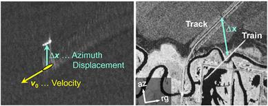
Figure 18.2 TerraSAR-X images of a moving ship in the Strait of Gibraltar (left) and a moving train near Wolgograd, Russia (right). The azimuth displacements can clearly be recognized.
For adding GMTI capabilities to SAR systems without preventing high resolution imaging appropriate techniques for suppressing the clutter are necessary. This can be achieved by implementing more than one receiving antenna or receiving channel. The signals received by multiple antennas, which are arranged in flight direction and which are separated by a certain baseline, can be combined in different ways: once for suppressing the clutter and so enabling the detection of even slowly moving targets, and once for estimating the motion and position parameters of the targets.
The question how many receiving antennas are needed can briefly be answered: for suppressing the clutter at least two receiving antennas separated by a certain baseline in azimuth or flight direction are necessary. A third antenna allows for a more robust estimation of the moving target’s true position and motion parameters. Additional antennas incorporate further degrees of freedom which for instance can be used for suppressing jammers [7]. This may be of importance for military applications. However, more than three antennas not necessarily improve the detection and parameter estimation performance significantly [8].
Today, GMTI is no longer limited to military applications. A SAR-GMTI system flying at high altitude can also be used for civilian wide area traffic monitoring, which has evolved into an important research topic during the last years [9–12]. Real-time traffic monitoring data for instance are used by traffic monitoring centers for ensuring the mobility and safety of the road users. Nowadays these data are mainly collected operationally from stationary sensors mounted along the major roads. Outside of these roads still a severe data lack exists, which even in short-term cannot fully be stuffed by the additional use of floating car data [13] and signaling information generated by the phone network. However, SAR-GMTI systems might be used in near future to fill these information gaps, especially if the information is required on a non-regular basis as in the case of major events and catastrophes.
Modern SAR-GMTI systems are expected to have at least the following capabilities:
• Detection of even slowly moving targets with low reflectivity (low RCS) against a strong clutter interference.
• Estimation of the moving targets’ true geographical positions.
• Estimation of the moving targets’ velocities and driving directions.
Furthermore, especially for military applications, it may also be required to
• Track the moving targets during the (increased) observation time.
• Refocus the “blurred” images of extended moving targets (an extended target is a target occupying more than one SAR resolution cell) like ships and larger land vehicles to high resolution for recognition purposes.
It has to be pointed out here that the latter three points will not be treated in this tutorial. Information about target tracking can e.g., be found in [14]. Refocusing of extended moving targets can be performed with inverse SAR (ISAR) imaging techniques. Adequate information and references can be found in [15–17] and also in the ISAR chapter of the ELSEVIER e-reference.
Principally two groups of multi-channel GMTI algorithms can be discriminated. The first group is based on the classical dual-channel techniques along-track interferometry (ATI) and displaced phase center antenna (DPCA). State-of-the-art spaceborne SAR systems limited to two physical receiving (RX) channels such as the German TerraSAR-X [6] and the Canadian RADARSAT-2 apply these GMTI techniques successfully. Thus, a special focus on these classical techniques is given in this tutorial. The second group is based on space-time adaptive processing (STAP) techniques for which a separate tutorial/chapter can be found in the ELSEVIER e-reference. For that reason only a short introduction to STAP is given in Sections 2.18.6.2.2 and 2.18.8.
For understanding the following sections of the tutorial the reader shall be familiar with the basic principles of SAR imaging. Good extended tutorials on SAR can for instance be found in [1] and in the SAR chapter of the ELSEVIER e-reference. As mathematical background mainly linear algebra (vectors and matrices), the understanding of the convolution and the Fourier transform and its inverse are required.
The remainder of this tutorial is organized as follows: in Section 2.18.2 the SAR principle is explained before in Section 2.18.3 the moving target single- and multi-channel signal model is derived. The effects caused by moving target signals are discussed in Section 2.18.4. They are fundamental for understanding the parameter estimation principles discussed afterwards. The classical dual-channel techniques are presented in detail in Section 2.18.5. In Section 2.18.6 the general GMTI processing chain is discussed and in Section 2.18.7 the basic Doppler parameter estimation methods are introduced. A short introduction to STAP is given in Section 2.18.8 before the tutorial is concluded with Section 2.18.9.
2.18.2 Synthetic aperture radar principle
For the following investigations a flat earth surface and a straight flight path of the SAR platform parallel to the earth surface are assumed. Although SAR and GMTI are not restricted to these assumptions (e.g., for spaceborne SAR-GMTI curved orbits have to be considered [18]), the explanations and equations given in the tutorial can be simplified to a certain degree and presented in a way better understandable by the interested reader who is not a SAR expert.
2.18.2.1 SAR acquisition geometry and operation
A SAR instrument consists of a pulsed transmitter, at least of one antenna which is used both for transmitting and receiving, and of a phase coherent receiver [1]. The typical side-looking imaging geometry of a SAR system is shown in Figure 18.3.
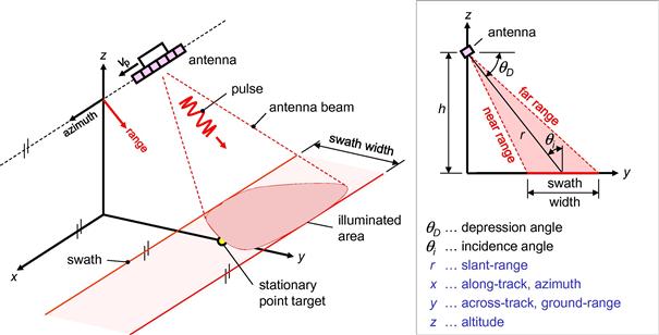
The platform carrying the radar instrument moves at constant altitude with constant velocity ![]() parallel to the x-axis. The moving direction of the radar is also denoted as along-track or azimuth direction. The antenna is mounted in a way so that the antenna beam with a certain depression angle
parallel to the x-axis. The moving direction of the radar is also denoted as along-track or azimuth direction. The antenna is mounted in a way so that the antenna beam with a certain depression angle ![]() points perpendicular to the azimuth direction towards the ground (the system in Figure 18.3 is left-looking with respect to the flight path). An area on ground with a certain swath width is illuminated by the beam. The radar is periodically emitting radar pulses of duration
points perpendicular to the azimuth direction towards the ground (the system in Figure 18.3 is left-looking with respect to the flight path). An area on ground with a certain swath width is illuminated by the beam. The radar is periodically emitting radar pulses of duration ![]() with the so called Pulse Repetition Frequency (PRF). The PRF typically is in the order of several 100 Hz (airborne systems) to several 1000 Hz (spaceborne systems). The pulses are backscattered from the illuminated area on ground, coherently received, down converted, digitized and stored in the mass memory of the SAR instrument. SAR processing is carried out afterwards, either onboard the platform or on ground after downloading the data.
with the so called Pulse Repetition Frequency (PRF). The PRF typically is in the order of several 100 Hz (airborne systems) to several 1000 Hz (spaceborne systems). The pulses are backscattered from the illuminated area on ground, coherently received, down converted, digitized and stored in the mass memory of the SAR instrument. SAR processing is carried out afterwards, either onboard the platform or on ground after downloading the data.
What the SAR measures are the backscattered signal energy and the time interval between the emitted and received pulses. The pulse travel time is proportional to the two-way range, i.e., the range from the antenna phase center to the target and back. A side-looking geometry is necessary so that for each measured slant range r the corresponding ground range or across-track position y can be computed unambiguously (cf. Figure 18.3).
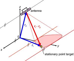
The SAR principle is based on a movement of the sensor with respect to the illuminated targets on ground. Due to the motion of the platform the range r between the platform and a specific stationary point target on ground changes as shown in Figure 18.4. This range change causes a Doppler frequency shift of the received signal which during SAR processing is exploited for synthesizing a large antenna along azimuth direction, resulting in a narrow synthetic azimuth beam width and, hence, in high azimuth resolution.

Due to the importance for GMTI processing discussed later, in the following the range and Doppler histories of the signal backscattered from a particular non-moving point target are derived.
The position of the antenna phase center located at the moving SAR platform with respect to the origin of the Cartesian {x, y, z} coordinate system can be written as (see also sketch in Figure 18.5)
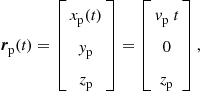 (18.5)
where ![]() is the constant platform velocity and t the time. At time
is the constant platform velocity and t the time. At time ![]() the platform is at altitude
the platform is at altitude ![]() above the origin of the Cartesian coordinate system. Let now the position of a certain non-moving “stationary” target be
above the origin of the Cartesian coordinate system. Let now the position of a certain non-moving “stationary” target be
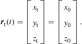 (18.6)
The indices “0” indicate time independent parameters. The distance between the antenna and the target can simply be computed as
![]() (18.7)
(18.7)
where ![]() denotes the
denotes the ![]() norm. For describing the SAR principle in common literature it is often assumed, without restriction of generality, that
norm. For describing the SAR principle in common literature it is often assumed, without restriction of generality, that ![]() so that at
so that at ![]() the point target is broadside the SAR platform. The minimum range
the point target is broadside the SAR platform. The minimum range ![]() at
at ![]() in this case can be written as
in this case can be written as
![]() (18.8)
(18.8)
so that (18.7) simplifies to
![]() (18.9)
(18.9)
The quadratic approximation given after the “![]() ” sign is obtained by a second-order Taylor expansion about
” sign is obtained by a second-order Taylor expansion about ![]() . The time t is proportional to the azimuth position of the platform
. The time t is proportional to the azimuth position of the platform ![]() :
:
![]() (18.10)
(18.10)
2.18.2.2 Stationary point target signal model
One single pulse transmitted by the SAR system can be expressed as
![]() (18.11)
(18.11)
where ![]() represents the pulse waveform in baseband,
represents the pulse waveform in baseband, ![]() is the so called “fast time,” j is the imaginary unit,
is the so called “fast time,” j is the imaginary unit, ![]() is the radar wavelength given by the carrier frequency and
is the radar wavelength given by the carrier frequency and ![]() denotes the speed of light in vacuum. Conventionally in SAR a linear frequency modulated (LFM) waveform, a so called “range chirp,” with a certain bandwidth
denotes the speed of light in vacuum. Conventionally in SAR a linear frequency modulated (LFM) waveform, a so called “range chirp,” with a certain bandwidth ![]() and a certain duration
and a certain duration ![]() (in the order of microseconds) is transmitted (although SAR is not limited to such waveforms). The range chirp in baseband is given as
(in the order of microseconds) is transmitted (although SAR is not limited to such waveforms). The range chirp in baseband is given as
 (18.12)
where ![]() denotes the chirp slope and
denotes the chirp slope and ![]() the envelope. The signal received from a point-like target is then a delayed and attenuated copy of the transmitted signal which can be written as
the envelope. The signal received from a point-like target is then a delayed and attenuated copy of the transmitted signal which can be written as
![]() (18.13)
(18.13)
The free-space attenuation, the backscattering coefficient, the elevation and the azimuth angles to the target as well as the weighting of the two-way antenna pattern are covered by the coefficient A. After coherent down-conversion to baseband using, e.g., a phase preserving quadrature demodulator, the received signal is given as
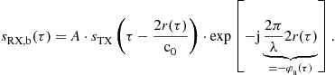 (18.14)
This signal can be separated into two parts:
1. The transmitted and delayed waveform ![]() whose delay is given by the two-way path 2
whose delay is given by the two-way path 2 ![]() between the antenna and the target.
between the antenna and the target.
2. An exponential term with phase ![]() representing the azimuth modulation of the signal, which is independent of the transmitted waveform.
representing the azimuth modulation of the signal, which is independent of the transmitted waveform.
The raw data signal given in (18.14) in its one-dimensional representation is in fact stored in a two-dimensional arrangement in the mass memory of the radar system according to the range and azimuth dimension. To get a better insight in this storage procedure one can make use of the start-stop-approximation. It assumes that the antenna and, hence, the SAR platform is motionless when a pulse is emitted and the scattered signal received. Afterwards the antenna moves to its next sending/receiving position along the flight track. This approximation can be made since the pulse travel time is much smaller than the time needed for the antenna to move to the next position. In range dimension the signal is sampled when the antenna is “motionless.” The range sampling frequency is determined by the analog-digital converter. For a complex signal this sampling frequency has to be at least as large as the chirp bandwidth ![]() so that the Nyquist criterion is not violated. In azimuth dimension the sampling frequency and, hence, the imaginary antenna “stops” are determined by the PRF.
so that the Nyquist criterion is not violated. In azimuth dimension the sampling frequency and, hence, the imaginary antenna “stops” are determined by the PRF.
The signal can therefore be written in a two-dimensional form as
![]() (18.15)
(18.15)
where ![]() is the “fast time” representing the range direction and t is the “slow time” representing the azimuth direction.
is the “fast time” representing the range direction and t is the “slow time” representing the azimuth direction.
Due to the importance for GMTI we will put the main focus on the azimuth signal
![]() (18.16)
(18.16)
where the rectangular function ![]() , defined e.g., in [3], is introduced for pointing out that the signal duration is limited by the illumination time
, defined e.g., in [3], is introduced for pointing out that the signal duration is limited by the illumination time ![]() given by the azimuth beamwidth of the antenna pattern. A small azimuth antenna length results in a wide beam (see also (18.1) and long illumination or synthetic aperture time, respectively. For typical airborne systems this time is in the order of several seconds, for state-of-the-art spaceborne systems around one second or smaller. The longer this time, the better is the achievable azimuth resolution after SAR processing.
given by the azimuth beamwidth of the antenna pattern. A small azimuth antenna length results in a wide beam (see also (18.1) and long illumination or synthetic aperture time, respectively. For typical airborne systems this time is in the order of several seconds, for state-of-the-art spaceborne systems around one second or smaller. The longer this time, the better is the achievable azimuth resolution after SAR processing.
The phase ![]() within the exponential term can according to (18.9) also be approximated using a second-order Taylor expansion, so that
within the exponential term can according to (18.9) also be approximated using a second-order Taylor expansion, so that
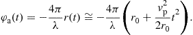 (18.17)
The azimuth phase modulation furthermore can be interpreted as azimuth frequency or Doppler frequency variation ![]() if the time derivative is taken in the following way:
if the time derivative is taken in the following way:
![]() (18.18)
(18.18)
If for the phase ![]() the quadratic approximation given in the second part of (18.17) is inserted, the linear approximation of the Doppler frequency history is obtained:
the quadratic approximation given in the second part of (18.17) is inserted, the linear approximation of the Doppler frequency history is obtained:
![]() (18.19)
(18.19)
It is obvious that the azimuth signal in the first approximation has the shape of a LFM signal with ![]() denoting the signal’s azimuth chirp slope or Doppler slope (see also Figure 18.4 bottom).
denoting the signal’s azimuth chirp slope or Doppler slope (see also Figure 18.4 bottom).
2.18.2.3 Pulse compression and image formation
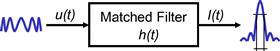
As mentioned in the previous section, the transmitted pulse typically has a time duration in the order of a few microseconds, whereas the illumination time of a particular point target is in the order of seconds. Thus, for achieving a high range and azimuth resolution pulse compression has to be employed. Pulse compression generally can be performed by convolving an uncompressed input signal u(t) with a proper reference function h(t). The pulse compressed signal I(t) in its general form is then given as
![]() (18.20)
(18.20)
where ![]() denotes convolution.
denotes convolution.
The optimal filter theory says that for signals embedded in white Gaussian noise the best signal-to-noise ratio (SNR) after convolution is achieved if the reference function h(t) is the complex conjugated and time reverted version of the “expected” input signal u(t):
![]() (18.21)
(18.21)
where ![]() is a constant which may be used for scaling purposes and
is a constant which may be used for scaling purposes and ![]() denotes the complex conjugation. If the reference function is constructed in this way, it is denoted as “Matched Filter” [19]. The resolution improvement by applying a matched filter is sketched in Figure 18.6. The comparatively long input signal u(t) after matched filtering is compressed to a pulse I(t) of short duration. The time resolution and, hence, the spatial resolution is significantly improved compared to the input signal.
denotes the complex conjugation. If the reference function is constructed in this way, it is denoted as “Matched Filter” [19]. The resolution improvement by applying a matched filter is sketched in Figure 18.6. The comparatively long input signal u(t) after matched filtering is compressed to a pulse I(t) of short duration. The time resolution and, hence, the spatial resolution is significantly improved compared to the input signal.
It is known that a cyclic convolution in time domain corresponds to a simple multiplication in frequency domain. For that reason the convolution in (18.20) can equivalently be written as
![]() (18.22)
(18.22)
where F and ![]() denote the Fourier and inverse Fourier transforms, respectively, and U( f ) and H( f ) are the frequency domain representations of u(t) and h(t), respectively.
denote the Fourier and inverse Fourier transforms, respectively, and U( f ) and H( f ) are the frequency domain representations of u(t) and h(t), respectively.
SAR processing or SAR image formation, within the GMTI community often denoted as “Stationary World Matched Filtering,” can be described briefly by the following three steps:
1. Range compression: A pulse compression along range dimension is performed. For the range chirp in (18.12) the reference function is
![]() (18.23)
(18.23)
2. Range cell migration correction (RCMC): The curvature of the range history is eliminated (see third image from left in Figure 18.7).

3. Azimuth compression: A pulse compression along azimuth is performed. For the azimuth signal in (18.16) the reference function is
![]() (18.24)
(18.24)
where the approximation after the “![]() ” sign is obtained by inserting the Taylor expansion from (18.17) into (18.16), substituting
” sign is obtained by inserting the Taylor expansion from (18.17) into (18.16), substituting ![]() and dropping the constant phase term
and dropping the constant phase term ![]() which is unimportant for pulse compression.
which is unimportant for pulse compression.
After performing these three steps a focused SAR image is obtained. These steps are visualized for a single point target in Figure 18.7. Details on state-of-the-art SAR processing algorithms and on the RCMC can e.g., be found in [3,20].
The focused image of a single point target is also denoted as impulse response function (IRF). The simulated IRF of a perfectly focused stationary point target is shown in Figure 18.8.
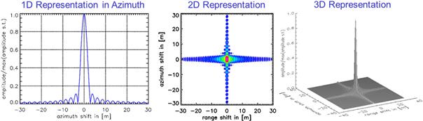
Figure 18.8 Impulse response function of a stationary point target (left: cut along azimuth direction; middle: two-dimensional representation; right: three-dimensional representation; system parameters: ![]() .
.
The IRF has the shape of a two-dimensional sinc function. The geometric resolution is determined by the 3 dB width of the IRF. The best achievable azimuth resolution is given in (18.4). If as transmitted waveform the LFM pulse given in (18.12) with a rectangular envelope ![]() is used, the best achievable range resolution is [3]
is used, the best achievable range resolution is [3]
![]() (18.25)
(18.25)
The larger the chirp bandwidth ![]() , the better is the range resolution.
, the better is the range resolution.
Due to the nature of SAR processing, the IRF of any target (independent whether it is moving or not) always is imaged at the position where the Doppler frequency of its uncompressed azimuth signal is zero. For a stationary target this position corresponds to the minimum range ![]() and to the actual azimuth position
and to the actual azimuth position ![]() . In contrast a moving point target, which is discussed in the next section, is displaced in azimuth and to a little extend in range, depending on the motion parameters. For investigating the displacements and additional effects the azimuth and range axis of the IRF plots shown in Figure 18.8, and in some of the Figures provided later in Section 2.18.4, are labeled as azimuth shift and range shift, respectively. The origins of the axes are centered around the positions
. In contrast a moving point target, which is discussed in the next section, is displaced in azimuth and to a little extend in range, depending on the motion parameters. For investigating the displacements and additional effects the azimuth and range axis of the IRF plots shown in Figure 18.8, and in some of the Figures provided later in Section 2.18.4, are labeled as azimuth shift and range shift, respectively. The origins of the axes are centered around the positions ![]() and
and ![]() . This has the advantage that the displacement quantities easily can be read off.
. This has the advantage that the displacement quantities easily can be read off.
2.18.3 Moving point target signal model
The obvious difference between a stationary and a moving point target is the position on ground, which varies over time depending on the target’s motion parameters. This time varying position difference results in a change of the range and Doppler histories and furthermore in some peculiar effects observable in the SAR images. For developing and understanding the fundamental moving target detection and parameter estimation principles and algorithms discussed later, it is first necessary to discuss suitable moving point target signal models. In the next two sections a single-channel as well as a multi-channel signal model are derived.
2.18.3.1 Single-channel signal model
In many of the publications related to GMTI a target in linear motion with constant acceleration during the observation time is assumed. This is especially for short observation times a valid assumption. Furthermore, it is assumed that the target does not change its altitude, i.e., that it does not move in z-direction. This is reasonable since the slopes of common roads only may cause a z-velocity component negligibly small compared to the large x- and y-components. The general acquisition geometry to consider is similar to that sketched in Figure 18.5, apart from the “stationary point target” which has to be replaced by a “moving point target.”
Under the afore mentioned assumption of linear motion the position of the moving point target (i.e., the motion equation) can in contrast to the stationary point target in (18.6) be written as
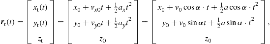 (18.26)
where ![]() , and
, and ![]() are the positions at
are the positions at ![]() and
and ![]() are the along-track and across-track velocity components at
are the along-track and across-track velocity components at ![]() , and
, and ![]() and
and ![]() are the constant along-track and across-track acceleration components. If the target moves during the illumination time along a straight line its position can also be expressed using the moving direction or road angle
are the constant along-track and across-track acceleration components. If the target moves during the illumination time along a straight line its position can also be expressed using the moving direction or road angle ![]() and the velocity and acceleration magnitudes
and the velocity and acceleration magnitudes ![]() and a (see right part of (18.26)). In this case the velocity and acceleration magnitudes are given as
and a (see right part of (18.26)). In this case the velocity and acceleration magnitudes are given as ![]() and
and ![]() . The moving direction
. The moving direction ![]() is measured counter-clockwise from the x-axis towards the y-axis as depicted in Figure 18.9.
is measured counter-clockwise from the x-axis towards the y-axis as depicted in Figure 18.9.
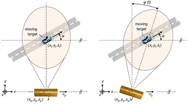
Figure 18.9 Target moving along a straight road section (left: non-squinted acquisition geometry; right: squinted acquisition geometry; the squint angle ![]() is measured from broadside direction in the slant range plane and its positive counting direction is clockwise).
is measured from broadside direction in the slant range plane and its positive counting direction is clockwise).
Even an acceleration change ![]() might be considered in the motion equations [21–23]. However, changing accelerations are neglected in this tutorial. They only play a significant role at long illumination times in the order of several seconds and for ISAR imaging purposes.
might be considered in the motion equations [21–23]. However, changing accelerations are neglected in this tutorial. They only play a significant role at long illumination times in the order of several seconds and for ISAR imaging purposes.
The position vector of the platform is the same as in (18.5). The range history ![]() of the moving target can then be written as
of the moving target can then be written as
 (18.27)
An analytical treatment of this expression is difficult because of the square root. For investigating effects on SAR imagery caused by moving targets it is appropriate to use the third-order Taylor expansion of the range history about ![]() which is given as
which is given as
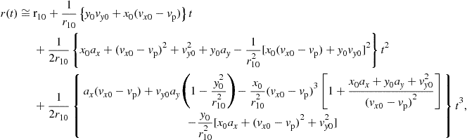 (18.28)
where the terms in the order of ![]() have been dropped. The range between the antenna and the target at
have been dropped. The range between the antenna and the target at ![]() is represented by
is represented by ![]() . In contrast to
. In contrast to ![]() in (18.8) the range
in (18.8) the range ![]() corresponds not to the range of closest approach since now the target is in motion and in the most general case not located at broadside position at
corresponds not to the range of closest approach since now the target is in motion and in the most general case not located at broadside position at ![]() (i.e.,
(i.e., ![]() ):
):
![]() (18.29)
(18.29)
With ![]() either a target track not centered in the azimuth beam or a squinted geometry as depicted in Figure 18.9 on the right can be considered. The target position
either a target track not centered in the azimuth beam or a squinted geometry as depicted in Figure 18.9 on the right can be considered. The target position ![]() at time
at time ![]() in this case can be expressed in terms of the squint angle
in this case can be expressed in terms of the squint angle ![]() of the antenna beam:
of the antenna beam: ![]() . If the squint angle
. If the squint angle ![]() is zero the antenna points perpendicular to the flight path so that
is zero the antenna points perpendicular to the flight path so that ![]() . A squint angle is either caused by a platform yaw due to crosswind or due to antenna beam steering. Typical squint angles caused by platform yaw are in the order of a few degrees. Thus, the
. A squint angle is either caused by a platform yaw due to crosswind or due to antenna beam steering. Typical squint angles caused by platform yaw are in the order of a few degrees. Thus, the ![]() terms in (18.28) as well as the
terms in (18.28) as well as the ![]() term have no significant contribution and therefore can be neglected. Also the
term have no significant contribution and therefore can be neglected. Also the ![]() term can be dropped so that the range equation for the moving target simplifies to
term can be dropped so that the range equation for the moving target simplifies to
 (18.30)
The azimuth phase of the moving target signal in the monostatic case (one common transmit (TX) and receiving (RX) antenna) is given by ![]() . The third-order Taylor expansion of the moving target’s Doppler frequency computed with (18.18) is then
. The third-order Taylor expansion of the moving target’s Doppler frequency computed with (18.18) is then
 (18.31)
where ![]() denotes the Doppler shift,
denotes the Doppler shift, ![]() the Doppler slope and q the quadratic Doppler coefficient.
the Doppler slope and q the quadratic Doppler coefficient.
By comparing (18.31) with (18.30) the approximated range history also can be expressed in terms of Doppler parameters:
![]() (18.32)
(18.32)
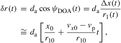
Using this range approximation the single-channel moving target azimuth signal can be written as
 (18.33)
where the constant phase determined by ![]() due to its unimportance has been dropped.
due to its unimportance has been dropped.
2.18.3.2 Multi-channel signal model
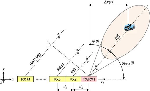
So far the range and Doppler histories of a moving target signal have been derived for the single-channel (monostatic) case where a common antenna is used for both TX and RX of the radar pulses. Now a system with M antennas is considered, where each antenna is separated from its neighbor in the along-track direction by a certain along-track baseline ![]() as depicted in Figure 18.10.
as depicted in Figure 18.10.
The first antenna is used for TX and RX, antenna 2 and all others for receive only. Following the derivation in [23] the ranges ![]() , for
, for ![]() can be written as
can be written as
 (18.34)
The range difference ![]() is given by [24]
is given by [24]
 (18.35)
where ![]() is the directional cosine measured from the x-axis. The expression after the “
is the directional cosine measured from the x-axis. The expression after the “![]() ” sign is the result of a first-order Taylor expansion. The multi-channel azimuth signals corresponding to the ranges in (18.34) are then
” sign is the result of a first-order Taylor expansion. The multi-channel azimuth signals corresponding to the ranges in (18.34) are then
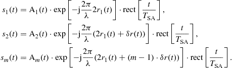 (18.36)
For the classical GMTI techniques ATI and DPCA treated in Section 2.18.5, the multi-channel azimuth signals in (18.36) need to be aligned or co-registered with the fore channel (![]() RX1) so that the antenna phase centers are at the same spatial location at different times. Thus, a shift of the signals is necessary. For co-registering with the signal
RX1) so that the antenna phase centers are at the same spatial location at different times. Thus, a shift of the signals is necessary. For co-registering with the signal ![]() the signal
the signal ![]() needs to be shifted by
needs to be shifted by ![]() , and
, and ![]() by
by ![]() .
.
For bistatic operation (only the fore antenna transmits, all others receive) the effective phase center separation is ![]() so that the time difference can be written as
so that the time difference can be written as
![]() (18.37)
(18.37)
The co-registered signals are then (to keep the equations shorter the ![]() functions have been omitted in the following)
functions have been omitted in the following)
 (18.38)
It can be shown that the range difference ![]() can be approximated as
can be approximated as
![]() (18.39)
(18.39)
and the range ![]() also can be written as [24]
also can be written as [24]
![]() (18.40)
(18.40)
with
![]() (18.41)
(18.41)
In practice all azimuth signals are sampled with a frequency given by the PRF. The sampling interval corresponds to ![]() so that e.g., the time discrete representation of the signals in (18.36) can be written as
so that e.g., the time discrete representation of the signals in (18.36) can be written as
![]() (18.42)
(18.42)
where N is the total number of azimuth samples. The received discrete azimuth signals (either un-registered or co-registered) can also be collected in a data matrix given as
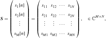 (18.43)
where M is the total number of receiving channels. Vectorizing (18.42) by stacking each succeeding column beneath the other yields
![]() (18.44)
(18.44)
where T means vector transposition.
2.18.4 Effects on SAR imagery
The first who has investigated the GMTI capabilities of SAR was Raney. In his fundamental paper from 1971 he already investigated the basic effects on SAR imagery caused by moving targets [5]. He found that a target motion parallel to the flight path of the radar results in a defocusing of the IRF and, hence, in a decreased peak amplitude and in a decreased signal-to-clutter-plus-noise ratio (SCNR). A motion perpendicular to the flight path causes an azimuth displacement of the target image proportional to the target’s across-track velocity. The understanding of these effects is fundamental for deriving appropriate moving target motion and position parameter estimation methods.
In the following sections the range cell migration, the residual range cell migration and the major effects caused by moving targets are discussed. As a starting point it is assumed that the signals are already range compressed in a perfect manner.
2.18.4.1 Residual range cell migration
Depending on the motion parameters the range histories of a moving target (18.30) and a stationary target (18.7) located at the same position at ![]() are quite different. Examples are shown in Figure 18.11, where the range history of a moving target signal1 (red) is compared with that of a stationary target (blue).
are quite different. Examples are shown in Figure 18.11, where the range history of a moving target signal1 (red) is compared with that of a stationary target (blue).
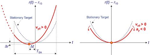
Figure 18.11 Influence of some motion parameters on the range history (left: influence of across-track velocity; right: influence of along-track velocity and across-track acceleration; the range history of the moving target signal is depicted in red color and the circle marks the moving target position after SAR focusing). (For interpretation of the references to color in this figure legend, the reader is referred to the web version of this book.)
If the target travels in across-track direction with a certain across-track velocity ![]() the range history is shifted in azimuth by
the range history is shifted in azimuth by ![]() and in range by
and in range by ![]() (Figure 18.11, left). The curvature itself is not changed significantly.
(Figure 18.11, left). The curvature itself is not changed significantly.
When the target travels in along-track direction or accelerates in across-track direction (Figure 18.11, right) the curvature is changed but the range history is not shifted. The range curvature change is equivalent to a quadratic phase error which after conventional SAR processing results in a blurred IRF.
A SAR processor performs a RCMC adapted only for stationary targets as depicted in the third image from the left in Figure 18.7. This RCMC is conventionally performed in the frequency domain [20]. For computing the residual range cell migration of the moving target signals it is necessary to express the range history as a function of Doppler frequency. The relation between time and Doppler frequency may be easily obtained from (18.31) if the quadratic Doppler coefficient q is neglected (for small illumination times the introduced error is negligibly small):
![]() (18.45)
(18.45)
By inserting this relationship in (18.32) the quadratic approximation of the moving target range history as a function of Doppler frequency is obtained:
![]() (18.46)
(18.46)
For a stationary target located at the same position as the moving target at time ![]() the quadratic approximation is
the quadratic approximation is
![]() (18.47)
(18.47)
where ![]() and
and ![]() are the Doppler parameters of the stationary target. These are obtained from (18.31) by setting the motion parameters
are the Doppler parameters of the stationary target. These are obtained from (18.31) by setting the motion parameters ![]() , and
, and ![]() to zero so that
to zero so that
![]() (18.48)
(18.48)
and
![]() (18.49)
(18.49)
For a non-squinted acquisition geometry ![]() and, hence,
and, hence, ![]() are zero.
are zero.
Since the SAR processor only performs the RCMC correctly for stationary targets a residual range cell migration ![]() remains for moving target signals. Its quadratic approximation is given as
remains for moving target signals. Its quadratic approximation is given as
 (18.50)
This expression is only valid for signals which are not aliased in Doppler. The residual range cell migration is the reason why the IRF of the moving target also may be blurred in range direction after azimuth compression. A detailed explanation on the range blur is given in Section 2.18.4.2.
An example for the residual range migration for an airborne system is shown in Figure 18.12.
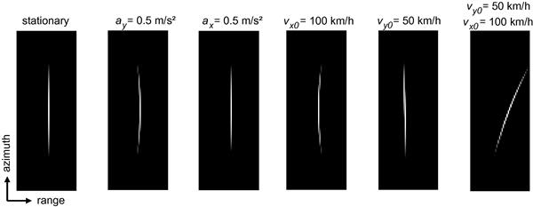
Figure 18.12 Simulated range compressed data after conventional RCMC adapted for stationary targets (simulation parameters: ![]() .
.
The results show that for targets accelerating in along-track direction (Figure 18.12, third image from the left) and for targets moving with constant velocity in across-track direction (second image from the right) almost no residual range cell migration exists. Thus, the major part of the signal energy is distributed along a single azimuth line. Such signals can easily be extracted from the range-compressed and RCMC data array for parameter estimation purposes discussed later.
A couple of years ago the so called “Keystone Transform” has been introduced with the aim to remove the linear range cell migration of the moving target signals, independent of their motion parameters [25]. However, the final result is the same as obtained by a conventional SAR processor based on chirp scaling [20] with omitted azimuth compression: the linear range cell migration of moving target signals is removed. Thus, if anyhow SAR processing is carried out the application of the Keystone transform is not necessary.
If the Doppler parameters ![]() and
and ![]() of a particular moving target signal are known (e.g., after estimation using proper techniques) a RCMC adapted to this target can be performed. An example is shown in Figure 18.13, where the same signals as for Figure 18.12 are used. In this case almost no residual range cell migration for the moving target signal remains. However, each moving target signal has different Doppler parameters and therefore requires the application of a different adapted RCMC which requires high computational power.
of a particular moving target signal are known (e.g., after estimation using proper techniques) a RCMC adapted to this target can be performed. An example is shown in Figure 18.13, where the same signals as for Figure 18.12 are used. In this case almost no residual range cell migration for the moving target signal remains. However, each moving target signal has different Doppler parameters and therefore requires the application of a different adapted RCMC which requires high computational power.

Figure 18.13 Simulated range compressed data after RCMC adapted for each target’s Doppler parameters (simulation parameters: ![]() .
.
With the proper moving target parameters additionally an adapted azimuth matched filter can be constructed so that a perfectly focused moving target image is obtained [26].
2.18.4.2 Along-track velocity
Equation (18.31) can be used for investigating the effects on the Doppler history. The major effect caused by the along-track velocity ![]() is a change of the Doppler slope
is a change of the Doppler slope ![]() with respect to the stationary target as sketched in Figure 18.14. Here
with respect to the stationary target as sketched in Figure 18.14. Here ![]() is the clutter bandwidth and
is the clutter bandwidth and ![]() is the illumination time.
is the illumination time.

Figure 18.14 Doppler history of a stationary target and a SWMF (left), and of a target moving either in along-track direction or accelerating in across-track direction (right). The Doppler history of the stationary target is shown in blue and of the moving target in red color. (For interpretation of the references to color in this figure legend, the reader is referred to the web version of this book.)
The Doppler slope change is equivalent to a change of the quadratic part of the range history. After azimuth compression using the SWMF with Doppler slope ![]() the mismatch
the mismatch ![]() corresponds to a quadratic phase error in time domain. The IRF of the moving target is therefore defocused in the azimuth direction as shown in Figure 18.15. Unfortunately no analytical description of the defocused IRF exists.
corresponds to a quadratic phase error in time domain. The IRF of the moving target is therefore defocused in the azimuth direction as shown in Figure 18.15. Unfortunately no analytical description of the defocused IRF exists.

Figure 18.15 Impulse response function of a simulated point target moving with constant velocity of ![]() in along-track direction, focused with SWMF (left: cut along azimuth; right: 2D representation; system parameters:
in along-track direction, focused with SWMF (left: cut along azimuth; right: 2D representation; system parameters: ![]() .
.
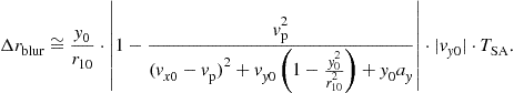
The spread of the blur in azimuth direction can be approximated as
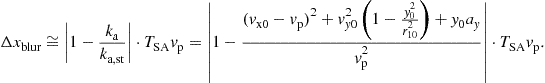 (18.51)
If the target only has an along-track velocity component (all other motion parameters are zero) for a system with ![]() (i.e., a spaceborne system) the simpler equation
(i.e., a spaceborne system) the simpler equation
![]() (18.52)
(18.52)
can be used [27]. This equation shows that the moving target is smeared by twice the distance it has moved in the along-track direction during the illumination time ![]() . The backscattered signal energy is distributed over a larger area. With increasing
. The backscattered signal energy is distributed over a larger area. With increasing ![]() the signal amplitude decreases as shown in Figure 18.15 left. A decreased signal amplitude leads to a decreased SCNR and a lower probability of detection. The target’s IRF additionally may be blurred in range due to the residual range cell migration.
the signal amplitude decreases as shown in Figure 18.15 left. A decreased signal amplitude leads to a decreased SCNR and a lower probability of detection. The target’s IRF additionally may be blurred in range due to the residual range cell migration.
For targets with ![]() (i.e., zero across-track velocity component) the spread of the blur in range direction can be computed using (18.50) and the relation
(i.e., zero across-track velocity component) the spread of the blur in range direction can be computed using (18.50) and the relation ![]() (non-squinted acquisition geometry assumed so that
(non-squinted acquisition geometry assumed so that ![]() and
and ![]() ):
):
 (18.53)
After inserting the Doppler parameters given in (18.31) and (18.49) as result
 (18.54)
is obtained. Especially for airborne systems the range blur may become significant. Let us assume for instance a system with ![]() and an extremely long illumination time
and an extremely long illumination time ![]() . In this case the range blur of the IRF of a target moving in along-track direction with 100 km/h (all other motion parameters are assumed to be zero) is 21 m. However, for spaceborne systems with
. In this case the range blur of the IRF of a target moving in along-track direction with 100 km/h (all other motion parameters are assumed to be zero) is 21 m. However, for spaceborne systems with ![]() and
and ![]() the range blur given in (18.53) and (18.54) can be neglected, especially under the aspect that the typical illumination time is in the order of one second.
the range blur given in (18.53) and (18.54) can be neglected, especially under the aspect that the typical illumination time is in the order of one second.
The relation between the range blur, the residual range cell migration and the motion parameters clearly can be recognized by looking again at Figure 18.12. Especially the across-track acceleration and the along-track velocity are the dominant motion parameters responsible for the quadratic phase errors (i.e., the mismatch with the Doppler slope of the SWMF) and, hence, for the residual range cell migration and the azimuth and range blur.
2.18.4.3 Across-track velocity
The major effect caused by the across-track velocity ![]() is a change of the Doppler shift
is a change of the Doppler shift ![]() given in (18.31). A secondary effect is a slight change of the Doppler slope
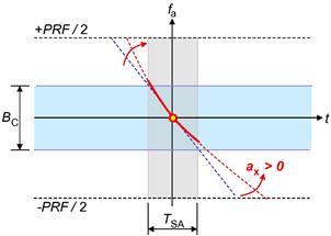
given in (18.31). A secondary effect is a slight change of the Doppler slope ![]() . In Figure 18.16 the Doppler history of a target moving in across-track direction is sketched. After SAR processing using the SWMF all targets, independent if stationary or moving, are imaged at the positions corresponding to their zero Doppler frequencies. For the moving target signal in Figure 18.16 this may either be the position marked with
. In Figure 18.16 the Doppler history of a target moving in across-track direction is sketched. After SAR processing using the SWMF all targets, independent if stationary or moving, are imaged at the positions corresponding to their zero Doppler frequencies. For the moving target signal in Figure 18.16 this may either be the position marked with ![]() or
or ![]() corresponds to the position of an ambiguity that is caused by an aliasing of the signal sampled by the PRF).
corresponds to the position of an ambiguity that is caused by an aliasing of the signal sampled by the PRF).

Figure 18.16 Doppler histories of a target moving in across-track direction (in red) and of the SWMF (in blue) (For interpretation of the references to color in this figure legend, the reader is referred to the web version of this book.).
The azimuth time ![]() where the target is imaged can be computed by setting (18.31) to zero and substituting
where the target is imaged can be computed by setting (18.31) to zero and substituting ![]() with
with ![]() for taking into account the Doppler slope of the SWMF. If only the quadratic approximation is used (the cubic coefficient q in (18.31) has been dropped since its contribution compared to the Doppler shift and Doppler slope is negligibly small) the following imaging time is obtained:
for taking into account the Doppler slope of the SWMF. If only the quadratic approximation is used (the cubic coefficient q in (18.31) has been dropped since its contribution compared to the Doppler shift and Doppler slope is negligibly small) the following imaging time is obtained:
![]() (18.55)
(18.55)
The imaging time corresponds to an along-track or azimuth displacement of
![]() (18.56)
(18.56)
For a non-squinted acquisition geometry (i.e., ![]() ) the equation simplifies to
) the equation simplifies to
![]() (18.57)
(18.57)
where ![]() , denoted as line-of-sight velocity, is the projection of the across-track velocity to the slant range direction. The relationship between the line-of-sight and the across-track velocity for a non-squinted geometry is given as
, denoted as line-of-sight velocity, is the projection of the across-track velocity to the slant range direction. The relationship between the line-of-sight and the across-track velocity for a non-squinted geometry is given as
![]() (18.58)
(18.58)
with ![]() being the incidence angle.
being the incidence angle.
The target is displaced in the flying direction (i.e., ![]() ) if it moves towards the radar (i.e.,
) if it moves towards the radar (i.e., ![]() ). It is displaced in opposite direction (i.e.,
). It is displaced in opposite direction (i.e., ![]() ) if it moves away from the radar (i.e.,
) if it moves away from the radar (i.e., ![]() ). In Figure 18.17 an IRF of a simulated point target moving with a constant velocity of 50 km/h in across-track direction is shown. It has a large azimuth displacement of about −978 m. Additionally the IRF is slightly shifted by −0.66 m in range direction (right image).
). In Figure 18.17 an IRF of a simulated point target moving with a constant velocity of 50 km/h in across-track direction is shown. It has a large azimuth displacement of about −978 m. Additionally the IRF is slightly shifted by −0.66 m in range direction (right image).

Figure 18.17 Impulse response function of a simulated point target moving with constant velocity ![]() in across-track direction, focused with SWMF (left: cut along azimuth; right: 2D representation; system parameters:
in across-track direction, focused with SWMF (left: cut along azimuth; right: 2D representation; system parameters: ![]() ).
).
The reason for the range displacement is the residual range cell migration. It can be computed with (18.50) by taking into account the fact that the major part of moving target’s signal energy is located around ![]() :
:
![]() (18.59)
(18.59)
For a non-squinted acquisition geometry (i.e., ![]() and
and ![]() ) the simplified expression
) the simplified expression
 (18.60)
can be used. The range displacement is always negative. Thus, a target with a non-zero across-track velocity component is always displaced towards the radar. The range displacements are small if compared to the azimuth displacements, especially for spaceborne systems. For instance, a fast target moving with a line-of-sight velocity of 100 km/h is displaced by only −5 m (typical low-earth orbit platform parameters ![]() and
and ![]() assumed). For airborne systems the displacement is larger. Here the same target is displaced by −143 m (
assumed). For airborne systems the displacement is larger. Here the same target is displaced by −143 m (![]() and
and ![]() assumed).
assumed).
As shown in Figure 18.17 the target’s IRF is severely displaced in azimuth but it is well focused. The slightly decreased peak amplitude is caused by the reduced spectral overlap of the SWMF with the moving target signal. The SWMF acts as a bandpass filter. Its Doppler bandwidth is conventionally limited to the clutter bandwidth ![]() given in (18.3). The reason for that is that the clutter for SAR imaging is the wanted signal. Everything outside the clutter bandwidth is uninteresting and therefore is filtered out. The extreme case is shown on the right side of Figure 18.16. Here no spectral overlap between the moving target signal shown in red and the bandwidth
given in (18.3). The reason for that is that the clutter for SAR imaging is the wanted signal. Everything outside the clutter bandwidth is uninteresting and therefore is filtered out. The extreme case is shown on the right side of Figure 18.16. Here no spectral overlap between the moving target signal shown in red and the bandwidth ![]() of the SWMF exists. As a consequence, fast moving targets are often not visible in conventional processed SAR images. To enable imaging and detection of fast moving targets the processing bandwidth of the SWMF has to be increased to the maximum possible bandwidth determined by the PRF. This is an important point to remember.
of the SWMF exists. As a consequence, fast moving targets are often not visible in conventional processed SAR images. To enable imaging and detection of fast moving targets the processing bandwidth of the SWMF has to be increased to the maximum possible bandwidth determined by the PRF. This is an important point to remember.
Due to the Doppler shift a part of the signal energy may be backfolded (i.e., aliased) so that ambiguities of the IRF appear at certain positions in the SAR image. On the left side of Figure 18.16, the primary IRF containing most of the signal energy is imaged at position ![]() whereas the ambiguity is imaged at
whereas the ambiguity is imaged at ![]() . To compute also the ambiguous target positions (18.56) can be extended to
. To compute also the ambiguous target positions (18.56) can be extended to
![]() (18.61)
(18.61)
An example of an ambiguous signal is shown in Figure 18.18.
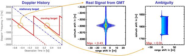
Figure 18.18 Impulse response of a simulated point target moving with high velocity in across-track direction with ![]() (left: Doppler history; middle: primary impulse response containing most of the energy; right: first ambiguity (note the different scale); system parameters:
(left: Doppler history; middle: primary impulse response containing most of the energy; right: first ambiguity (note the different scale); system parameters: ![]() .
.
To keep the ambiguities at a low level commonly a high PRF should be chosen. To ensure that at least half of the signal energy of a point target lies within the PRF band its Doppler shift has to be smaller than ![]() . Using this requirement with (18.31) and again assuming for simplicity a non-squinted geometry (i.e.,
. Using this requirement with (18.31) and again assuming for simplicity a non-squinted geometry (i.e., ![]() ) the upper bound for the across-track velocity is
) the upper bound for the across-track velocity is
![]() (18.62)
(18.62)
This bound ensures that at least half of the signal energy is unambiguously available. The equation can be considered as a criterion for selecting the minimum required PRF of a SAR-GMTI system depending on the highest “expected” target across-track velocity:
![]() (18.63)
(18.63)
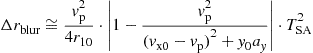
For targets with ![]() (i.e., for targets moving with a certain across-track velocity) the spread of the range blur can be approximated as (
(i.e., for targets moving with a certain across-track velocity) the spread of the range blur can be approximated as (![]() and
and ![]() assumed)
assumed)
![]() (18.64)
(18.64)
With the inserted Doppler parameters given in (18.31) this results in
 (18.65)
If for instance an airborne system with ![]() , and
, and ![]() would be used the IRF of a target moving in across-track direction with 50 km/h (all other motion parameters are assumed to be zero) has a range blur of 0.05 m. For state-of-the-art airborne SAR systems this is below the achievable range resolution and therefore can be neglected. However, if aside of the across-track velocity of 50 km/h also an along-track velocity component of 100 km/h is considered, the range blur increases to 52 m.
would be used the IRF of a target moving in across-track direction with 50 km/h (all other motion parameters are assumed to be zero) has a range blur of 0.05 m. For state-of-the-art airborne SAR systems this is below the achievable range resolution and therefore can be neglected. However, if aside of the across-track velocity of 50 km/h also an along-track velocity component of 100 km/h is considered, the range blur increases to 52 m.
2.18.4.4 Along-track acceleration
The major effect of the along-track acceleration ![]() is a change of the quadratic coefficient q in (18.31) which causes a deflection of the Doppler history as sketched in Figure 18.19.
is a change of the quadratic coefficient q in (18.31) which causes a deflection of the Doppler history as sketched in Figure 18.19.
After azimuth compression the IRF of the moving target has a decreased peak amplitude and shows non-symmetric (unbalanced) sidelobes. The strength of this effect depends mainly on the synthetic aperture time ![]() . The longer this time the larger are the third-order phase errors in time domain and the more severe the effect. An example for an airborne system is shown in Figure 18.20.
. The longer this time the larger are the third-order phase errors in time domain and the more severe the effect. An example for an airborne system is shown in Figure 18.20.

Figure 18.20 Impulse response functions of a simulated point target accelerating in along-track direction, focused with SWMF (left: the bandwidth of the SWMF was 100 Hz corresponding to an integration time of about 1 s; right: bandwidth of 600 Hz corresponding to about 6 s integration time; system parameters: ![]() .
.
For spaceborne SAR systems with typical illumination times below one second the effects caused by the along-track acceleration are negligibly small.
2.18.4.5 Across-track acceleration
The across-track acceleration ![]() causes a similar major effect as the along-track velocity
causes a similar major effect as the along-track velocity ![]() : a change of the Doppler slope
: a change of the Doppler slope ![]() given in (18.31) (see also Figure 18.14). This results again in a blurred IRF with decreased peak amplitude. The IRF looks similar as the response shown in Figure 18.15 and is therefore not separately depicted. The azimuth blur caused by the across-track acceleration can be derived with (18.51). If all other target motion parameters are zero it is given as
given in (18.31) (see also Figure 18.14). This results again in a blurred IRF with decreased peak amplitude. The IRF looks similar as the response shown in Figure 18.15 and is therefore not separately depicted. The azimuth blur caused by the across-track acceleration can be derived with (18.51). If all other target motion parameters are zero it is given as
![]() (18.66)
(18.66)
Even an allegedly small acceleration my cause a azimuth blur in the order of several meters. For an airborne system with ![]() , and
, and ![]() an acceleration of
an acceleration of ![]() results in an azimuth blur of approximately 15 m. For a spaceborne system with
results in an azimuth blur of approximately 15 m. For a spaceborne system with ![]() , and
, and ![]() the azimuth blur is 4.5 m. Neither for airborne nor for high resolution spaceborne SAR systems this effect should be neglected. By measuring the spread of the azimuth blur of the moving target’s IRF the effects caused by across-track accelerations and along-track velocities cannot be separated.
the azimuth blur is 4.5 m. Neither for airborne nor for high resolution spaceborne SAR systems this effect should be neglected. By measuring the spread of the azimuth blur of the moving target’s IRF the effects caused by across-track accelerations and along-track velocities cannot be separated.
Additionally to the azimuth blur the IRF is also blurred in range. The range blur caused by the across-track acceleration can be computed with (18.54). Using the same parameters for an airborne and spaceborne system as before, the range blurs caused by an acceleration of ![]() are 0.6 m and 7 mm. Thus, at least for the spaceborne system, the range blur can be neglected.
are 0.6 m and 7 mm. Thus, at least for the spaceborne system, the range blur can be neglected.
2.18.4.6 Summary of effects
The effects treated so far caused by moving targets on SAR imagery are summarized in Table 18.1. The knowledge of these effects and their origins are fundamental for developing suitable GMTI systems and algorithms [9].
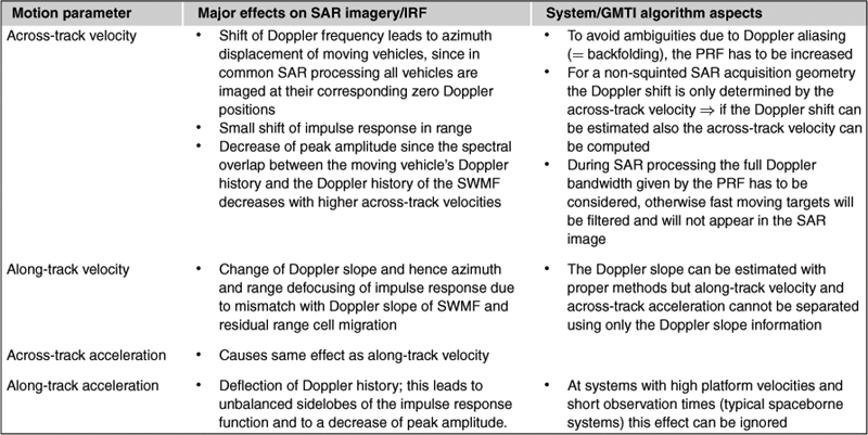
2.18.5 Classical dual-channel techniques
In the following two sections the classical dual-channel techniques are discussed. They principally can be applied on raw data, range compressed data and fully focused data.
2.18.5.1 Along-track interferometry
For along-track interferometry (ATI) two receiving antennas displaced in azimuth direction by a certain baseline ![]() are necessary. The receiving antennas can either be mounted on the same platform or on separate platforms flying in formation along the same track (separate platforms allow for larger baselines). Anyhow, each antenna observes the scene from the same point in space at slightly different times
are necessary. The receiving antennas can either be mounted on the same platform or on separate platforms flying in formation along the same track (separate platforms allow for larger baselines). Anyhow, each antenna observes the scene from the same point in space at slightly different times ![]() and
and ![]() . During the time lag
. During the time lag ![]() the signals from stationary targets remain the same whereas the signals from targets moving in range direction experience a phase shift
the signals from stationary targets remain the same whereas the signals from targets moving in range direction experience a phase shift ![]() . This phase shift is called ATI phase. It is proportional to the line-of-sight velocity of the moving target. The time lag
. This phase shift is called ATI phase. It is proportional to the line-of-sight velocity of the moving target. The time lag ![]() has to be sufficiently short to avoid the effect of temporal decorrelation caused by slight changes in the scene (e.g., due to wind) between the acquisitions of an interferometric image pair. The first application of ATI was oceanography where it was used to measure tidal currents with a velocity estimation accuracy in the order of several cm/s [28].
has to be sufficiently short to avoid the effect of temporal decorrelation caused by slight changes in the scene (e.g., due to wind) between the acquisitions of an interferometric image pair. The first application of ATI was oceanography where it was used to measure tidal currents with a velocity estimation accuracy in the order of several cm/s [28].
The ATI principle is sketched in Figure 18.21. At time ![]() the target is observed by the fore antenna at range
the target is observed by the fore antenna at range ![]() . At time
. At time ![]() it is observed by the aft antenna at a different range
it is observed by the aft antenna at a different range ![]() . The range difference
. The range difference ![]() (t) is proportional to the ATI phase. The ATI signal is computed by multiplying the signal of the fore antenna with the complex conjugate and co-registered signal of the aft antenna (remember the co-registered multi-channel signals given in (18.38):
(t) is proportional to the ATI phase. The ATI signal is computed by multiplying the signal of the fore antenna with the complex conjugate and co-registered signal of the aft antenna (remember the co-registered multi-channel signals given in (18.38):
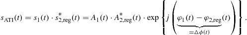 (18.67)
If both channels are well calibrated and the RCS of the target does not change between both observations the complex coefficients ![]() and
and ![]() are identical (i.e., same phases and amplitudes), so that the ATI phase may be computed as:
are identical (i.e., same phases and amplitudes), so that the ATI phase may be computed as:
![]() (18.68)
(18.68)
The phases of both signals are given as
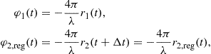 (18.69)
with ![]() where
where ![]() is the antenna phase center separation in along-track direction (= effective along-track baseline). If both antennas receive and transmit independently (= monostatic operation) the phase center separation corresponds to the physical antenna separation, i.e.,
is the antenna phase center separation in along-track direction (= effective along-track baseline). If both antennas receive and transmit independently (= monostatic operation) the phase center separation corresponds to the physical antenna separation, i.e., ![]() . In case of bistatic operation where only the fore antenna is used for transmission but both antennas for signal reception the effective along-track baseline reduces to half the physical distance, i.e.,
. In case of bistatic operation where only the fore antenna is used for transmission but both antennas for signal reception the effective along-track baseline reduces to half the physical distance, i.e., ![]() .
.
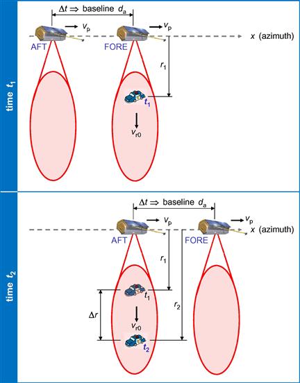
By inserting (18.69) in (18.68) the ATI phase may be written as
![]() (18.70)
(18.70)
If the target moves with constant line-of-sight velocity ![]() the ATI phase of the target at broadside position for monostatic operation in the simplest case can be approximated as (the squint angle and all other motion parameters of the target are assumed to be zero) [28]
the ATI phase of the target at broadside position for monostatic operation in the simplest case can be approximated as (the squint angle and all other motion parameters of the target are assumed to be zero) [28]
![]() (18.71)
(18.71)
If the line-of-sight velocity is computed from the measured ATI phase blind velocities and ambiguities may occur. The reason is that the ATI phase can only be measured in fractions of 2![]() . A blind velocity occurs if the measured ATI phase becomes zero. This is the case for
. A blind velocity occurs if the measured ATI phase becomes zero. This is the case for
![]() (18.72)
(18.72)
The blind velocities can be computed by inserting (18.71) in the previous equation:
![]() (18.73)
(18.73)
If the target moves with a blind velocity its ATI phase cannot be discriminated from the ATI phase of a stationary target and, hence, it cannot be detected in the interferogram.
An ambiguity occurs if the ATI phase is equal or larger than ![]() . In this case neither the motion direction (away or towards the radar) nor the velocity can be determined unambiguously. The maximum line-of-sight velocity causing no ambiguities is given as (again derived with (18.71))
. In this case neither the motion direction (away or towards the radar) nor the velocity can be determined unambiguously. The maximum line-of-sight velocity causing no ambiguities is given as (again derived with (18.71))
![]() (18.74)
(18.74)
The maximum line-of-sight velocity can be increased by using larger radar wavelengths ![]() or smaller time lags
or smaller time lags ![]() (i.e., smaller baselines).
(i.e., smaller baselines).
In Figure 18.22 a polar plot of an azimuth line of interest containing a moving target signal is shown. The azimuth line was focused with the SWMF before the polar plot was generated. Several dots in the polar plot belong to the target since it spans multiple resolution cells. It also can be seen that the target dots have slightly different phases. The reason is that the target is not perfectly focused (remember the potential mismatch of the Doppler slope of the target and the SWMF). Furthermore, since ATI performs no clutter suppression also the clutter contribution disturbing the ATI phase clearly can be recognized. As a consequence the ATI phases of moving target signals are biased towards zero so that velocities are generally underestimated. For low SCNR values this bias is more significant.
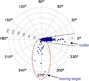
Figure 18.22 Polar plot of ATI phases of an extracted azimuth line containing a moving target signal. The data was acquired with DLR’s airborne sensor E-SAR.
Even if there is no temporal decorrelation and if the clutter would be suppressed somehow prior to ATI phase computation, the minimum detectable velocity (MDV) and the accuracy of the line-of-sight velocity estimate is limited by the thermal receiver noise. The receiver noise in both RX channels causes a phase decorrelation which results in a noisy estimate of the ATI phase. The amplitude of the complex correlation coefficient due to thermal receiver noise between both channels is given as [29]
![]() (18.75)
(18.75)
where SNR is the signal-to-noise ratio after SAR focusing (i.e., after pulse compression). The standard deviation of the ATI phase for point-like scatterers for values of ![]() close to one can be approximated as [30,31]
close to one can be approximated as [30,31]
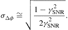 (18.76)
This equation can be considered as a lower bound of the ATI phase standard deviation. For extended objects (i.e., targets larger than a single SAR resolution cell) the standard deviation is larger but it can be reduced to a certain degree by ATI phase averaging (=multi-looking).
The lower bound of the standard deviation of the line-of-sight velocity computed with (18.71) and (18.75) can be expressed as
![]() (18.77)
(18.77)
The standard deviation of the azimuth position computed using (18.56) is then
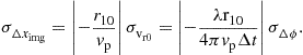 (18.78)
By having a closer look at (18.77) and (18.78) it is obvious that the standard deviation can be decreased by increasing the time lag ![]() and, hence, the antenna phase center separation
and, hence, the antenna phase center separation ![]() . However, it has to be kept in mind that by increasing
. However, it has to be kept in mind that by increasing ![]() the maximum unambiguously detectable line-of-sight velocity in (18.74) and the blind velocities in (18.73) decrease. Techniques for phase unwrapping are necessary if the motion and position parameters of faster moving targets shall be estimated with high accuracy. Promising candidates are for instance multi-baseline ATI techniques [32,33]. Ambiguities might also be resolved if the range cell migration of the target is exploited for a rough line-of-sight velocity estimation which afterwards is refined with the information obtained from the ATI phase [21]. For large time lags, temporal decorrelation may also have a negative influence, but this aspect is not treated here.
the maximum unambiguously detectable line-of-sight velocity in (18.74) and the blind velocities in (18.73) decrease. Techniques for phase unwrapping are necessary if the motion and position parameters of faster moving targets shall be estimated with high accuracy. Promising candidates are for instance multi-baseline ATI techniques [32,33]. Ambiguities might also be resolved if the range cell migration of the target is exploited for a rough line-of-sight velocity estimation which afterwards is refined with the information obtained from the ATI phase [21]. For large time lags, temporal decorrelation may also have a negative influence, but this aspect is not treated here.
Figure 18.23 shows the standard deviations of the line-of-sight velocity and the azimuth position for exemplary airborne and spaceborne acquisition geometries. It is obvious that with airborne systems even with small baselines in the fraction of a meter good estimation results can be achieved. For spaceborne systems comparatively large baselines are required to push down the standard deviations and, hence, to improve the parameter estimation accuracy. However, the size and weight of SAR satellites are limited by launcher restrictions. For instance, the German TerraSAR-X satellite has an antenna length of 4.8 m which can be split into two RX sub-apertures of 2.4 m each. In bistatic operation (i.e., TX with full antenna and RX with both halves simultaneously) the phase center separation or the effective along-track baseline, respectively, is only 1.2 m. For high SNR values of 20 dB the azimuth position estimation accuracy is in the order of 150 m. The accuracy decreases to 490 m if the SNR decreases to 10 dB. Compared to airborne systems, state-of-the-art spaceborne systems generally achieve worse position and motion parameter estimation accuracies. The two main reasons are the too short baselines and the worse SNR values.
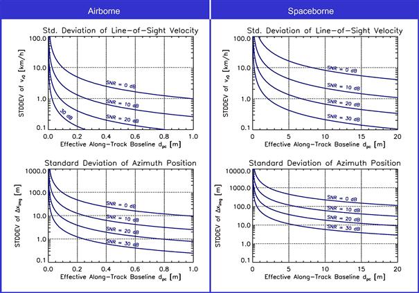
Figure 18.23 Standard deviations of the estimates of line-of-sight velocity and azimuth position for an exemplary airborne (left) and spaceborne (right) SAR acquisition geometry (airborne parameters: ![]() ; spaceborne parameters:
; spaceborne parameters: ![]() .
.
For an in-depth ATI performance analysis also the clutter contribution has to be considered [34, 35]. However, for understanding the basic ATI principles and performance limitations the previous explanations are sufficient.
In reality a moving target seldom has only a line-of-sight velocity component with all other motion components being zero as assumed in the derivation of (18.71). Although ATI is primarily sensitive to the line-of-sight velocity ![]() also the other motion components contribute to the ATI phase. Unfortunately there exists no analytical description for the ATI signal focused with a SWMF. However, if the Doppler slope of the matched filter used for azimuth compression is adapted to the Doppler slope
also the other motion components contribute to the ATI phase. Unfortunately there exists no analytical description for the ATI signal focused with a SWMF. However, if the Doppler slope of the matched filter used for azimuth compression is adapted to the Doppler slope ![]() of the target an analytical solution exists (matched filters adapted to target motion’s parameters are discussed in Section 2.18.7.1). In case of a non-squinted geometry (i.e.,
of the target an analytical solution exists (matched filters adapted to target motion’s parameters are discussed in Section 2.18.7.1). In case of a non-squinted geometry (i.e., ![]() and
and ![]() ) the ATI phase of the peak of the refocused target signal is given as [23]
) the ATI phase of the peak of the refocused target signal is given as [23]
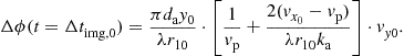 (18.79)
The ATI phase depends not only on the across-track velocity ![]() but also on the along-track velocity
but also on the along-track velocity ![]() . This has to be taken into account for accurate parameter estimation.
. This has to be taken into account for accurate parameter estimation.
2.18.5.2 Displaced phase center antenna technique
The displaced phase center antenna (DPCA) technique is one of the simplest clutter suppression techniques in radar [36]. The antenna configuration is exactly the same as in ATI: at least two receiving antennas are needed (see also Figure 18.21). The only difference is the signal processing. Instead of a complex conjugate multiplication the co-registered signal received by the aft antenna is subtracted from the signal received by the fore antenna for obtaining the DPCA signal
![]() (18.80)
(18.80)
Signals from stationary targets are canceled since they are identical in both successive observations. Targets moving with sufficient line-of-sight velocity cause a certain phase shift and, thus, will not be canceled. As a consequence even slowly moving targets otherwise masked by the clutter can be detected in the “clutter-suppressed” DPCA image. If the clutter is homogeneous DPCA can be considered as the optimal linear filter for target detection [37]. Although DPCA originally was developed for dual-channel systems, it also can be used with more than two channels [38–40].
In older literature it is often stated that the so called “DPCA Condition” has to be fulfilled. That means that the PRF has to be selected in a way that the spatial location of the fore antenna phase center when an echo is received is the same as the location of the aft antenna phase center when the next echo is received:
![]() (18.81)
(18.81)
Nowadays this restriction is relaxed. By modern signal processing techniques co-registration can be performed with sub-sample accuracy using interpolation or resampling, respectively. Often the co-registration is done by applying a phase ramp on the signal after transforming it via an FFT to the Doppler domain (remember the displacement law of the Fourier transform). The phase ramp to be applied in Doppler domain for co-registration along azimuth generally is given as
![]() (18.82)
(18.82)
This leads to accurate co-registration results as long as the Nyquist sample theorem is fulfilled for both clutter and moving target signals. In other words, a sufficiently high PRF is required for avoiding aliasing of signals in Doppler. However, if the PRF is too low the aliased clutter signals after co-registration have a constant phase error [18]. A coarse co-registration without interpolation can be done by shifting the data by an integer amount of samples. The time in (18.82) for fine co-registration with sub-sample accuracy can then be decreased to ![]() ). The constant phase error derived in [18] in this case can be written as
). The constant phase error derived in [18] in this case can be written as
![]() (18.83)
(18.83)
Due to this constant phase error aliased clutter might be mistaken as false moving targets. Especially for spaceborne systems the Doppler bandwidth is large compared to the PRF so that Doppler aliasing cannot be excluded. It generally is more severe than in airborne systems. Therefore, for spaceborne systems it is advisable to meet the DPCA condition in (18.81) as accurate as possible so that no phase ramp in Doppler for fine-co-registration needs to be applied. In this case ![]() is zero and the phase error in (18.83) vanishes.
is zero and the phase error in (18.83) vanishes.
For achieving a good detection performance it is essential that the receiving channels are well calibrated. For calibration the “Adaptive 2D Channel Balancing” method originally proposed by Ender [7] has established itself in the GMTI community. The method operates in the 2D frequency domain. The channel transfer functions are adapted to a reference channel, conventionally the fore channel. The method is not limited to two channels. Also co-registration is performed between the channels since any phase ramps in frequency domain are removed [41]. In Figure 18.24 an example with three moving targets is shown. It can be seen that after channel balancing (right column) the SCNR as well as the correlation coefficient ![]() is increased. Even targets with lower RCS are clearly visible in the balanced DPCA image. Theoretically the clutter can be suppressed down to noise level. The application of a channel balancing method is absolutely crucial, especially for airborne GMTI algorithms based on classical ATI and DPCA.
is increased. Even targets with lower RCS are clearly visible in the balanced DPCA image. Theoretically the clutter can be suppressed down to noise level. The application of a channel balancing method is absolutely crucial, especially for airborne GMTI algorithms based on classical ATI and DPCA.
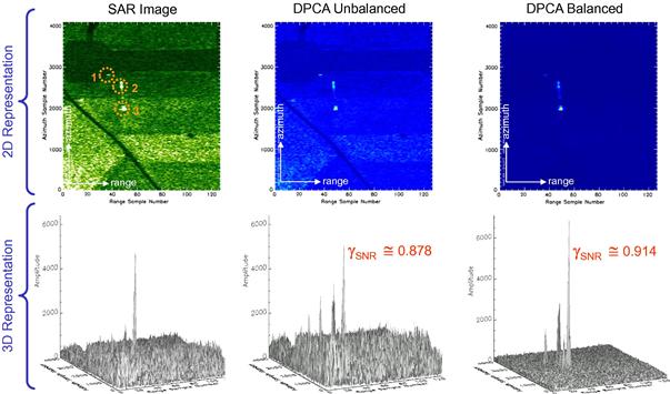
Figure 18.24 Clutter suppression capabilities of unbalanced DPCA and balanced DPCA (left column: single-channel airborne SAR image containing three targets moving in range direction; middle: DPCA image generated from unbalanced two-channel data; right: DPCA image generated from balanced data).
If the channels are well calibrated so that ![]() , the DPCA signal can also be expressed as
, the DPCA signal can also be expressed as
![]() (18.84)
(18.84)
where ![]() is the phase of the complex coefficient
is the phase of the complex coefficient ![]() . For detecting a moving target the magnitude of the DPCA signal is of interest:
. For detecting a moving target the magnitude of the DPCA signal is of interest:
![]() (18.85)
(18.85)
If the target moves with constant line-of-sight velocity ![]() (all other motion parameters are zero) the DPCA magnitude can be approximated as
(all other motion parameters are zero) the DPCA magnitude can be approximated as
![]() (18.86)
(18.86)
It is obvious that the DPCA magnitude drops to zero if the sine becomes zero. This is the case if the target moves with a blind velocity given in (18.73). Thus, neither with ATI nor with DPCA targets moving with blind velocities can be detected.
2.18.6 General GMTI processing chain
In this section the general GMTI processing chain is presented and discussed. Figure 18.25 shows a simplified flow chart containing the typical GMTI processing steps. At the very first beginning the acquired radar data in their raw form are necessary as input. These data somehow need to be preprocessed before the “GMTI Kernel” can be applied.

The “GMTI Kernel” represents a general GMTI algorithm with the processing steps: clutter suppression, detection, signal extraction, and parameter estimation. Principally every state-of-the-art GMTI algorithm consists of these steps. However, the steps are not always clearly separable and the step order may be different. Especially “Signal Extraction” sometimes is not necessary.
In the following sections the different steps are explained.
2.18.6.1 Preprocessing
As input for a SAR-GMTI processor single- or multi-channel raw data acquired with air- or spaceborne sensors are used. These data need to be preprocessed (step 2 in Figure 18.25) before the “GMTI Kernel” can be applied. Depending on the particular GMTI algorithm to be used in the “GMTI Kernel” several preprocessing options are conceivable (no claim to completeness):
2.18.6.1.1 Range compression
The acquired data are only compressed in range, no RCMC and no azimuth compression is carried out. This kind of preprocessing is used especially for airborne GMTI algorithms based on STAP [4,37]. Most of these algorithms use only short integration times so that range cell migration can be neglected. Large SNR values are required since due to the low sample support the compression gain obtained by coherent integration is limited. However, with state-of-the-art airborne systems this is not a problem in contrast to spaceborne systems which have to cope with comparatively low SNR values.
2.18.6.1.2 Range compression with RCMC
The data are range compressed and a RCMC is performed. The RCMC may either be adapted to stationary targets, as done during conventional SAR processing, or in an iterative way to some of the moving target’s motion parameters. A detailed discussion on RCMC and residual range cell migration was already given in Section 2.18.4.1 and shall not be repeated here.
2.18.6.1.3 Conventional SAR processing
The data are processed with a conventional SAR processor, e.g., a Range/Doppler [3] or a Chirp Scaling Processor [20]. The full Doppler bandwidth given by the PRF has to be considered to avoid filtering of signal energy of fast moving targets (cf. Section 2.18.4.3).
2.18.6.1.4 Motion adapted SAR processing
The data are processed iteratively using different assumptions of target’s motion parameters. This kind of preprocessing requires high computational power. However, the advantage is that high SCNR values may be achieved. This especially is crucial for spaceborne systems which generally suffer from low SNR and SCNR values (cf. Section 2.18.5.1).
2.18.6.2 Clutter suppression
Most of the multi-channel GMTI algorithms found in the literature use either DPCA or STAP techniques for clutter suppression.
2.18.6.2.1 DPCA
Dual-channel algorithms mainly use the DPCA technique discussed in Section 2.18.5.2 for clutter suppression. This technique can also be used if more than two RX channels are available [38,39]. For instance several clutter suppressed image pairs can be generated using DPCA. The ATI phase between these image pairs is then less influenced by clutter [42]. This improves the moving target parameter estimation accuracy significantly. In the ideal case the clutter is suppressed down to noise level so that the curves shown in Figure 18.23 apply for the velocity and position estimation accuracy.
In the general case the clutter filtered signal ![]() is obtained by a linear combination of the received multi-channel signal or space-time snapshot
is obtained by a linear combination of the received multi-channel signal or space-time snapshot ![]() with the clutter filter or weight vector
with the clutter filter or weight vector ![]()
![]() (18.87)
(18.87)
where H denotes complex conjugate transposition (i.e., Hermitian transpose) [43]. The clutter and noise contaminated space-time snapshot ![]() has the same array structure as the multi-channel signal vector
has the same array structure as the multi-channel signal vector ![]() given in (18.44). The dimension is
given in (18.44). The dimension is ![]() , where M is the number of receiving antennas and N the number of considered temporal samples.
, where M is the number of receiving antennas and N the number of considered temporal samples.
If multi-channel DPCA using M antennas shall be applied for clutter suppression, the weight vector is given as [43]
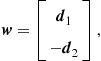 (18.88)
where ![]() and
and ![]() are the M-dimensional spatial-only steering vectors for the first and second pulses (i.e.,
are the M-dimensional spatial-only steering vectors for the first and second pulses (i.e., ![]() ), respectively. The steering vectors are then
), respectively. The steering vectors are then
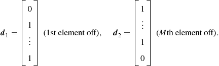 (18.89)
It has to be noted that in this case the DPCA condition has to be fulfilled. The data must not be co-registered. The output of the clutter filter is a scalar if only two temporal samples are used. To filter an entire azimuth line the filter has to be applied successively, each time using two temporal samples.
2.18.6.2.2 Adaptive clutter suppression
In the multi-channel case adaptive clutter filtering can be performed by multiplying the acquired and preprocessed multi-channel signal with the inverse of the clutter covariance matrix and a steering vector [4,37]. The adaptive weight vector is formed in the following way
![]() (18.90)
(18.90)
where ![]() is the clutter covariance matrix of dimension
is the clutter covariance matrix of dimension ![]() and
and ![]() is the steering vector.
is the steering vector.
The clutter covariance matrix itself can either be computed analytically using the known system, antenna and geometry parameters or, more powerfully, be estimated from the real data (it is then called “Empirical Clutter Covariance Matrix” or “Sample Clutter Covariance Matrix”). In the latter case the clutter covariance matrix is “adapted” to the real “clutter” data. The processing is then called “Space-Time Adaptive Processing (STAP)” (see also Section 2.18.9). The empirical clutter covariance matrix can be computed by averaging training data which shall not contain moving target signals [4]:
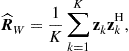 (18.91)
where ![]() is the
is the ![]() vector of training data from training cell k, and K is the total number of used training cells. The averaging for instance could be performed over range as exemplarily sketched in Figure 18.26. To exclude potential moving target signals a guard zone should be used [43,44].
vector of training data from training cell k, and K is the total number of used training cells. The averaging for instance could be performed over range as exemplarily sketched in Figure 18.26. To exclude potential moving target signals a guard zone should be used [43,44].

If again two successive temporal samples (N = 2) and as steering vector
 (18.92)
are used, then the clutter suppression method is called “Adaptive DPCA” (ADPCA) [44].
2.18.6.3 Detection
Conventionally moving targets are detected on a pixel by pixel basis. A threshold is set to discriminate between one of the two hypotheses ![]() (moving target signal not present) and
(moving target signal not present) and ![]() (moving target signal present):
(moving target signal present):
![]() (18.93)
(18.93)
where ![]() denotes the vector of the received data,
denotes the vector of the received data, ![]() is the clutter vector and
is the clutter vector and ![]() the noise vector.
the noise vector.
Generally a so called “Constant False Alarm Rate (CFAR)” detector is envisaged. The threshold is computed in a way that the percentage of the image pixels which lie above the threshold is constant. For computation the clutter statistics have to be known precisely.
If the probability density function (PDF) of the clutter is known, the false alarm rate or the probability of a false alarm is obtained by integrating the PDF:
![]() (18.94)
(18.94)
where ![]() is the threshold and
is the threshold and ![]() the PDF of the clutter metric to be tested (e.g., the clutter DPCA amplitude, the clutter ATI phase, the clutter ATI phase combined with the clutter ATI amplitude, etc.). If a certain false alarm rate is desired this equation needs to be solved for the threshold
the PDF of the clutter metric to be tested (e.g., the clutter DPCA amplitude, the clutter ATI phase, the clutter ATI phase combined with the clutter ATI amplitude, etc.). If a certain false alarm rate is desired this equation needs to be solved for the threshold ![]() . Depending on
. Depending on ![]() an analytical solution is not always possible so that numerical methods may be necessary.
an analytical solution is not always possible so that numerical methods may be necessary.
The probability of detection can be expressed as
![]() (18.95)
(18.95)
where ![]() is the target plus interference PDF.
is the target plus interference PDF.
Analytical descriptions of the PDFs of the clutter multi-look ATI phase and ATI amplitude can be found in [34]. In that paper different clutter types are modeled and verified with real data. A discrimination between homogeneous (Gaussian), heterogeneous (non-Gaussian) and extremely heterogeneous clutter is made. A novel polynomial PDF called p-distribution is introduced. This PDF matches the real data much more accurately, particularly for heterogeneous composite terrain. All clutter parameters for determining the detection thresholds are estimated from the real data. Further detection metrics are discussed in [45]. Here also a so called “Hyperbolic Detector” well suited for heterogeneous terrain such as urban areas is introduced.
For estimating the clutter statistics from the real data the moving target itself has to be excluded. This can be achieved by introducing a guard zone around the pixel under test as depicted in Figure 18.27. The clutter statistics is then estimated from the data surrounding the guard zone. The purpose of the guard zone is to exclude that moving target signal components disturb the clutter and, hence, lead to a wrong clutter PDF estimate. The size of the guard zone shall be chosen in accordance with the expected sizes of the moving vehicles to be detected. If the guard zone is too small or if a lot of targets move close together, the clutter PDF estimate is biased and the false alarm rate will not remain constant anymore.

For studying and comparing the performance of different detector types as quality measures the probability of detection ![]() versus varying SCR and
versus varying SCR and ![]() versus
versus ![]() can be used [46]. The latter quality measure is known as receiver operating characteristics (ROC) of a detector. Since the exact PDF of the target signal is generally unknown, it is conventionally assumed to be either deterministic or Gaussian distributed.
can be used [46]. The latter quality measure is known as receiver operating characteristics (ROC) of a detector. Since the exact PDF of the target signal is generally unknown, it is conventionally assumed to be either deterministic or Gaussian distributed.
2.18.6.4 Signal extraction
Once a moving target has been detected it is of interest to estimate its motion and position parameters. For that purpose the moving target signal may be extracted from the data. An extraction also may be required if for instance the target image shall be refocused to high resolution using ISAR imaging techniques [15–17]. In the following two practicable extraction methods are discussed.
2.18.6.4.1 Range history tracking
The principle is depicted in Figure 18.28 on the left. The method operates on range compressed data where the clutter already has been canceled. Each pixel corresponding to the clutter suppressed moving target signal has to be detected (the detected pixels are represented by the pink squares in the image). The aligned pixels represent the moving target azimuth signal s(t) which afterwards can be passed to the parameter estimation stage. The range history tracking method was introduced in [47]. A detailed description of the “tracking” algorithm is given in [21].
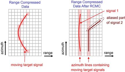
Figure 18.28 Moving target signals in the range compressed SAR data array (left: range compressed data without RCMC; right: range compressed data after conventional RCMC for stationary targets).
The method has the advantage that even signals backfolded in Doppler can be tracked and that information about the shape of the range history is obtained (remember in particular the influence of the across-track velocity on the range history shape discussed in Section 2.18.4.1). The disadvantage is that the clutter suppressed signal must have high SCNR values to be detectable on a pixel-by-pixel basis. This restricts the application to airborne GMTI. Tracking might also become problematic if several targets with overlapping range histories are in the data array.
2.18.6.4.2 Extraction of azimuth lines
The principle of the azimuth line extraction method is sketched in Figure 18.28 on the right. The data have to be range compressed and also the range cell migration has to be corrected, at least with respect to stationary targets. Depending on the motion parameters and on the range pixel spacing (which is determined by the range sampling rate) a major part of the signal energy may be distributed along a single azimuth line (see also discussion on residual range cell migration in Section 2.18.4.1). Thus, by extracting the proper azimuth line the signal ![]() is obtained. The method can also be applied prior to the detection step. Then all azimuth lines of the data are successively extracted. Afterwards detection and parameter estimation are carried out using different methods discussed later.
is obtained. The method can also be applied prior to the detection step. Then all azimuth lines of the data are successively extracted. Afterwards detection and parameter estimation are carried out using different methods discussed later.
From signals backfolded in Doppler only a part of the signal energy can be recovered. The “aliased part” is lost if the RCMC was adapted for stationary targets (cf. Figure 18.28, right). Successive preprocessing with different motion adapted RCMC may help to catch more signal energy and avoid aliasing [39,48]. Anyhow, the simple extraction of azimuth lines is a very fast method which also works for signals with low SCNR as in the case of spaceborne GMTI. Furthermore, even multi-target scenarios (i.e., if more than one moving target signal is contained in the extracted azimuth line) can be resolved by using e.g., a matched filter bank or the fractional Fourier transform discussed later in Sections 2.18.7.1 and 2.18.7.2, respectively.
Also from fully focused SAR images the azimuth lines can be extracted. However, before applying a matched filter bank the azimuth compression has to be removed (this can simply be done by adapting the reference function of the matched filter).
2.18.6.5 Parameter estimation
In (18.31) it is shown that the target’s motion parameters are related to the Doppler parameters shift ![]() , slope
, slope ![]() , and quadratic coefficient q. Thus, motion parameter estimation can be reduced to Doppler parameter estimation. From the known Doppler parameters the position and motion parameters of the moving target can be computed. The intention of this section is to show how this computation is principally performed by different state-of-the-art GMTI algorithms. In the following it is supposed that the Doppler slope
, and quadratic coefficient q. Thus, motion parameter estimation can be reduced to Doppler parameter estimation. From the known Doppler parameters the position and motion parameters of the moving target can be computed. The intention of this section is to show how this computation is principally performed by different state-of-the-art GMTI algorithms. In the following it is supposed that the Doppler slope ![]() and shift
and shift ![]() already have been estimated. Basic Doppler parameter estimation methods are discussed afterwards in Section 2.18.7.
already have been estimated. Basic Doppler parameter estimation methods are discussed afterwards in Section 2.18.7.
It is also supposed that the radar parameters and the acquisition geometry are known accurately so that the parameters ![]() , and
, and ![]() need not to be estimated. This is a valid assumption, particularly if the range is large compared to a potential range displacement
need not to be estimated. This is a valid assumption, particularly if the range is large compared to a potential range displacement ![]() (i.e.,
(i.e., ![]() . Additionally a non-squinted acquisition geometry is assumed (i.e.,
. Additionally a non-squinted acquisition geometry is assumed (i.e., ![]() and
and ![]() ).
).
2.18.6.5.1 Across-track velocity
The relation between the Doppler shift and the across-track velocity is given in (18.31). In case of a non-squinted acquisition geometry the simple relationship
![]() (18.96)
(18.96)
applies. However, in practice the across-velocity is computed from the estimated ATI phase ![]() . In the simplest case the relationship given in (18.71) is used so that the across-track velocity computes to
. In the simplest case the relationship given in (18.71) is used so that the across-track velocity computes to
![]() (18.97)
(18.97)
To mitigate the influence of clutter and to keep the estimation bias at a low level the moving target’s IRF should be refocused before estimating the ATI phase (refocusing increases the SCNR). More robust algorithms exploit three RX channels for ATI phase estimation as sketched in Figure 18.29. They generate two DPCA images: the first by subtracting channel 2 from 1, and the second by subtracting channel 3 from 2. The corresponding clutter suppressed ATI signal is then obtained by
![]() (18.98)
(18.98)
This has the advantage that the clutter is suppressed theoretically down to noise level so that in the best case the performance limits depicted in Figure 18.23 can be reached.
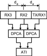
One promising state-of-the-art GMTI algorithm which additionally uses the fractional Fourier transform (explained in detail in Section 2.18.7.2) for target refocusing and additional parameter estimation is presented in [35]. An extension to spaceborne geometries can be found in [18]. Here also different transmit and receiver aperture switching strategies for generating additional receiving channels with larger baselines are discussed. Especially for spaceborne systems larger baselines are of importance for improving the parameter estimation accuracy.
2.18.6.5.2 Along-track velocity
Remember (18.31) where it is shown that the Doppler slope ![]() depends on the along-track velocity
depends on the along-track velocity ![]() , the across-track acceleration
, the across-track acceleration ![]() and on the across-track velocity
and on the across-track velocity ![]() in the following way:
in the following way:
 (18.99)
Under the assumption that the across-track velocity ![]() can be estimated with ATI still two unknowns remain:
can be estimated with ATI still two unknowns remain: ![]() and
and ![]() . Without further information the two unknowns cannot be computed. This is just the crux of many GMTI algorithms which exploit only the Doppler slope. Since the required additional information cannot be gained accelerations are assumed to be negligibly small. They are simply set to zero. The along-track velocity is derived by rearranging (18.99)
. Without further information the two unknowns cannot be computed. This is just the crux of many GMTI algorithms which exploit only the Doppler slope. Since the required additional information cannot be gained accelerations are assumed to be negligibly small. They are simply set to zero. The along-track velocity is derived by rearranging (18.99)
 (18.100)
where incorrectly the term ![]() is ignored by many GMTI algorithms. However, this assumption is in reality only valid if an across-track motion can be excluded a priori. Thus, the target must move only in along-track direction for avoiding estimation errors.
is ignored by many GMTI algorithms. However, this assumption is in reality only valid if an across-track motion can be excluded a priori. Thus, the target must move only in along-track direction for avoiding estimation errors.
In [49] it is shown that the typical standard deviation of the acceleration of a common passenger car is in the order of 0.5 m/s![]() . For TerraSAR-X a comparatively small across-track acceleration of 0.25 m/s
. For TerraSAR-X a comparatively small across-track acceleration of 0.25 m/s![]() would lead, if neglected in (18.100), to an along-track velocity estimation error of −32 km/h. This demonstrates clearly that accelerations should not be neglected if highly accurate velocity parameter estimates are desired.
would lead, if neglected in (18.100), to an along-track velocity estimation error of −32 km/h. This demonstrates clearly that accelerations should not be neglected if highly accurate velocity parameter estimates are desired.
In the literature so far only two algorithms can be found which take into account the accelerations for parameter estimation. Both of them don’t use the estimated Doppler slope for along-track velocity estimation. They use a different measure not influenced by across-track accelerations.
The algorithm in [50] was developed for a single-channel SAR but can principally also be used in the multi-channel case. It exploits the fact that the effective synthetic aperture time and, hence, the Doppler bandwidth varies with the moving target’s along-track velocity. Thus, by estimating the Doppler bandwidth of the extracted moving target signal the along-track velocity can be computed without the negative influence of accelerations in the following way:
![]() (18.101)
(18.101)
where ![]() is the length of the synthetic aperture for a stationary target located at the same range, and
is the length of the synthetic aperture for a stationary target located at the same range, and ![]() is the estimated Doppler bandwidth of the moving target signal. The drawback of the algorithm is that it only works properly for strong point-like targets with a RCS that is independent of the aspect angle. Furthermore, the whole target signal energy has to be collected since otherwise the Doppler bandwidth cannot be estimated accurately.
is the estimated Doppler bandwidth of the moving target signal. The drawback of the algorithm is that it only works properly for strong point-like targets with a RCS that is independent of the aspect angle. Furthermore, the whole target signal energy has to be collected since otherwise the Doppler bandwidth cannot be estimated accurately.
In [24] the ATI phase history of range compressed moving target signals between two or more receiving channels which are not co-registered is exploited. The slope of the ATI phase history is given as
![]() (18.102)
(18.102)
It is not influenced by accelerations. Thus, by estimating the slope the along-track velocity ![]() can be computed as
can be computed as
![]() (18.103)
(18.103)
The method is suitable for airborne systems where the SNR is generally much higher than in satellite systems. A good performance can be achieved for signals with SCNR values larger than 10 dB.
Both methods discussed before require large SCNR values to achieve a good along-track velocity estimation accuracy. Therefore they are not well suited for spaceborne systems. They should always be used supplementary to methods exploiting the Doppler slope.
2.18.6.5.3 Accelerations
The estimation of target accelerations is generally of minor interest. The reason why accelerations are still of importance is that they may improve the velocity estimation accuracy.
The across-track acceleration can be computed by rearranging (18.99):
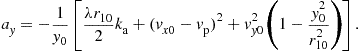 (18.104)
The along-track acceleration principally can be computed by rearranging the equation of the quadratic Doppler coefficient which is given as:
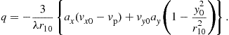 (18.105)
However, for estimating q long observation times are necessary. At short observation times q is negligibly small and cannot be estimated precisely (cf. also Section 2.18.4.4 where the effect caused by the along-track acceleration is discussed).
2.18.6.5.4 True target position
As discussed in Section 2.18.4.3 a target moving in across-track direction appears displaced from its actual position in the SAR image. It is displaced in azimuth as well as in range direction.
It is shown in (18.57) that the along-track displacement is directly related to the across-track velocity ![]() in the following way:
in the following way:
![]() (18.106)
(18.106)
Thus, once the across-track velocity is estimated (e.g., with ATI) the azimuth displacement can be computed. The same is valid for the range displacement given in (18.60).
Another interesting dual-channel method for estimating the broadside position, which corresponds to the true target position in the non-squinted case, is presented in [51]. Here again the ATI phase history of range compressed signals which are not co-registered is exploited. The distances between the target and the fore and the aft antenna phase centers are exactly equal if the target is located broadside. Thus, by estimating the zero crossing of the ATI phase history the broadside position and, hence, the true target position can be computed. Since the ATI phase history is strongly influence by clutter bandpass filtering in the fractional Fourier domain is performed. The effectiveness of this filtering is illustrated in Figure 18.30 (the zero crossing is at ![]() ). The method can also be used with more than two channels by additionally using DPCA for clutter suppression [24]. Also the ATI phase slope for computing the along-track velocity can be estimated as discussed in Section 2.18.6.5.2.
). The method can also be used with more than two channels by additionally using DPCA for clutter suppression [24]. Also the ATI phase slope for computing the along-track velocity can be estimated as discussed in Section 2.18.6.5.2.

Figure 18.30 Unregistered ATI phase history (blue: without clutter suppression; yellow: clutter suppressed using bandpass filtering in fractional Fourier domain) [24] (For interpretation of the references to color in this figure legend, the reader is referred to the web version of this book.)
A third method for estimating the true target positions are displacement based algorithms. These algorithms require the incorporation of a priori knowledge about the road network. The along-track displacement ![]() can then simply be measured: it is the distance between the position where the target is imaged and the road axis (cf. Figure 18.31). For a spaceborne system the range displacement
can then simply be measured: it is the distance between the position where the target is imaged and the road axis (cf. Figure 18.31). For a spaceborne system the range displacement ![]() is only in the order of a few meters and therefore can be neglected (cf. Section 2.18.4.3). The along-track displacement estimation accuracy is mainly related to the position accuracy of the road axis and the road width. From the estimated displacement easily the across-track velocity can be derived:
is only in the order of a few meters and therefore can be neglected (cf. Section 2.18.4.3). The along-track displacement estimation accuracy is mainly related to the position accuracy of the road axis and the road width. From the estimated displacement easily the across-track velocity can be derived:
![]() (18.107)
(18.107)
Since also the road angle ![]() is available from the road database the along-track velocity can be computed as
is available from the road database the along-track velocity can be computed as ![]() . The across-track acceleration is obtained with (18.104) after the Doppler slope
. The across-track acceleration is obtained with (18.104) after the Doppler slope ![]() has been estimated. For computing the along-track acceleration again the road angle can be used so that
has been estimated. For computing the along-track acceleration again the road angle can be used so that ![]() . Although all important motion parameters can be derived the displacement based algorithms have one major disadvantage: problems may arise if a lot of adjacent roads are located in the scene. Then the detected targets under circumstances cannot be assigned to the correct roads.
. Although all important motion parameters can be derived the displacement based algorithms have one major disadvantage: problems may arise if a lot of adjacent roads are located in the scene. Then the detected targets under circumstances cannot be assigned to the correct roads.

An operational traffic monitoring algorithm for TerraSAR-X based on the displacement technique is presented in [11,52].
2.18.6.6 Visualization
Finally, the detected target can be visualized. Often a symbol representing the moving target is overlaid on the corresponding SAR image on its estimated position. For instance, the symbol may be an arrow pointing into the estimated moving direction and the color of this symbol may correspond to the velocity. An example for such a visualization is shown in Figure 18.32.

Figure 18.32 Single-channel SAR image with three detected moving targets (location: airfield in Memmingen, Germany; data acquired with DLR’s E-SAR sensor) [53].
Another elegant possibility for visualization is Google Earth. The parameters of the detected moving targets are written into a Keyhole Markup Language (KML) file. Also links to target symbols and SAR images can be incorporated easily. The KML file can then be visualized with Google Earth as shown in Figure 18.33.
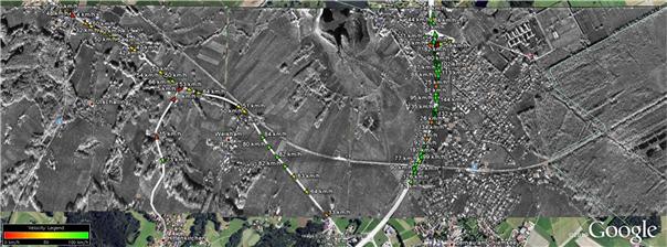
Figure 18.33 SAR image and detected moving targets as Google Earth overlay (location: near Chiemsee, Germany; scene size ![]() ; data acquired with DLR’s F-SAR sensor). Some of the slower moving targets are false detections.
; data acquired with DLR’s F-SAR sensor). Some of the slower moving targets are false detections.
Furthermore, additional information about the detected target can be provided in an interactive way. The user or operator can click on the moving target symbols to open a window. This window may contain more information about the detected target. Also data from additional data sources can be incorporated and fused with the SAR data. For instance, the estimated parameters of detected ships could be fused with “ground truth” data obtained from the automatic identification system (AIS) [54]. An example is depicted in Figure 18.34. Such ground truth data can also be used for evaluating the parameter estimation accuracy of GMTI algorithms.
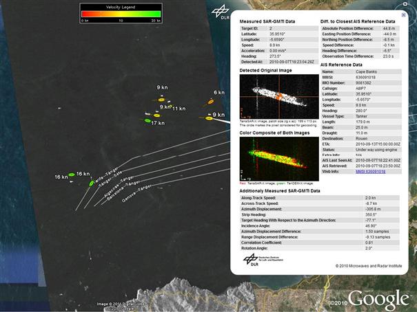
Figure 18.34 Google Earth image of the Strait of Gibraltar overlaid with the KML file obtained from the TerraSAR-X/TanDEM-X large along-track baseline GMTI processor [55]. The color coded symbols (color is velocity dependent) mark the estimated “true” geographical positions of the automatically detected ships, also the displaced ship images in white color are visible.
2.18.7 Doppler parameter estimation: basic methods
The intention of this section is to introduce the fundamental and most promising Doppler parameter estimation methods which are used in state-of-the-art GMTI algorithms. Most of these methods can even be used for both target detection and parameter estimation in one step.
For estimating the Doppler shift ![]() which is mainly related to the across-track velocity the ATI technique discussed in Sections 2.18.5.1 and 2.18.6.5.1 can be used. The Doppler slope
which is mainly related to the across-track velocity the ATI technique discussed in Sections 2.18.5.1 and 2.18.6.5.1 can be used. The Doppler slope ![]() for instance can be estimated by using a matched filter bank, the fractional Fourier transform or the Wigner-Ville distribution in combination with the Radon transform. Due to their importance they are discussed in detail.
for instance can be estimated by using a matched filter bank, the fractional Fourier transform or the Wigner-Ville distribution in combination with the Radon transform. Due to their importance they are discussed in detail.
In the following explanations for simplicity the single-channel moving point target signal model is used. However, the application of the presented detection and parameter estimation methods is not limited to the single-channel case. The methods also can be applied on clutter suppressed multi-channel signals almost without restrictions.
2.18.7.1 Matched filter bank
The basic principle of a matched filter was discussed in Section 2.18.2.3. It was shown that a signal can be focused by performing a convolution with a proper reference function. Also a moving target signal can perfectly be focused if the proper reference function is applied [21]. The proper azimuth reference function for focusing the moving target signal is given as
![]() (18.108)
(18.108)
However, the Doppler parameters ![]() , and q are unknown in advance. They need to be estimated. This can be done by convolving the range compressed moving target signal successively with different azimuth reference functions. For each of these functions different Doppler parameter are assumed. The estimated Doppler parameters
, and q are unknown in advance. They need to be estimated. This can be done by convolving the range compressed moving target signal successively with different azimuth reference functions. For each of these functions different Doppler parameter are assumed. The estimated Doppler parameters ![]() , and
, and ![]() are obtained from the reference function that after convolution results in the highest peak value of the IRF. The successive convolution with different reference functions is called “Matched Filter Bank” and can be considered as a maximum likelihood estimator for the Doppler or motion parameters [56].
are obtained from the reference function that after convolution results in the highest peak value of the IRF. The successive convolution with different reference functions is called “Matched Filter Bank” and can be considered as a maximum likelihood estimator for the Doppler or motion parameters [56].
Principally the moving target signal has to be extracted from the range compressed data array before the matched filter bank can be applied [47]. For this task the range history tracking method presented in Section 2.18.6.4.1 can be used for example. However, as a brute force method also two-dimensional matched filters can be constructed taking additionally into account the range history of the target signal. Each (pre-detected) pixel of the range compressed data array has then to be convolved with a set of two-dimensional matched filters. One can conceive that this method has a high computational load and is rather time consuming. However, the method may be of importance for spaceborne systems which suffer from low SNR values. The advantages are the higher compression gain and the possibility to estimate the parameters from fast moving targets aliased in Doppler [57]. The minimum PRF requirement given in (18.62) is not applicable in this case. A lower PRF resulting in less range ambiguities can be used. Additionally, the swath width (cf. Figure 18.3) of the SAR system can be increased [1] by lowering the PRF.
The moving target signal can also be extracted “by chance” using the method discussed in Section 2.18.6.4.2. With this method successive azimuth lines are extracted. The disadvantage is that no direct information about the range history is preserved. In this case the matched filter bank is not very sensitive to the Doppler shift ![]() . However, the Doppler shift or equivalently the across-track velocity can be estimated using ATI. If additionally the quadratic coefficient q is neglected (it only has a significant contribution at large observation times) a much simpler azimuth reference function can be used:
. However, the Doppler shift or equivalently the across-track velocity can be estimated using ATI. If additionally the quadratic coefficient q is neglected (it only has a significant contribution at large observation times) a much simpler azimuth reference function can be used:
![]() (18.109)
(18.109)
The equivalent in Doppler domain is given as
![]() (18.110)
(18.110)
It has to be kept in mind that with this reference function only the Doppler slope ![]() of the moving target signal can be estimated. After focusing with this reference function the target still appears displaced from its actual position.
of the moving target signal can be estimated. After focusing with this reference function the target still appears displaced from its actual position.
An example of the application of a matched filter bank on real dual-channel airborne data is shown in Figure 18.35. On the left side a SAR image containing four targets moving on a runway with different along-track velocities is shown. Target 2 moved with 10 km/h. The azimuth line containing “Target 2” was extracted from the clutter suppressed DPCA image and the azimuth compression was removed. Afterwards the matched filter bank was applied. The matched filter bank output, denoted as “Matched Filter Map,” is shown on the right, once in its two-dimensional representation and once in its 3D representation. The target is represented by the focused peak. The peak position corresponds to a certain estimated Doppler slope and to a certain azimuth position. In the example the target moved only in along-track direction (![]() and
and ![]() ) so that with (18.100) the along-track velocity
) so that with (18.100) the along-track velocity ![]() can be computed easily (the negative sign in the image is due to the antiparallel motion with respect to the flight path).
can be computed easily (the negative sign in the image is due to the antiparallel motion with respect to the flight path).
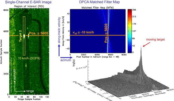
Figure 18.35 Application of a matched filter bank on an extracted azimuth line (left: single-channel SAR image acquired with DLR’s E-SAR sensor [58]; top right: 2D representation of the matched filter bank output; bottom: 3D representation of the output).
As already explained, the application of the matched filter bank is not limited to azimuth lines containing only one moving target signal. In fact a multi-target scenario can be resolved as shown in the example depicted in Figure 18.36. Here an azimuth line of interest containing a part of the Autobahn A8 near Chiemsee, Germany, where several targets have moved was extracted. In the SAR image on the left the targets are severely blurred in azimuth and cannot be recognized and separated. However, in the matched filter map of the DPCA signal each target appears as a focused peak at a certain azimuth and Doppler slope position. Thus, a matched filter bank not only can be used for parameter estimation, but also for target detection and target separation. It can deal with multi-component LFM signals. Target detection in the matched filer map either can be performed by applying a certain amplitude threshold or by comparing the sharpness of the peaks with analytical sharpness functions [27].

2.18.7.2 Fractional Fourier transform
The fractional Fourier transform (FrFT) is a linear operator (no cross-terms in case of multi-component LFM signals) and can be considered as a generalization (or rotation with rotation angle ![]() of the conventional Fourier transform [59]. The FrFT has found many applications like swept-frequency filters, time-variant filtering and multiplexing, pattern recognition and the study of time-frequency distributions. It is also known, that the Radon transform [60] of the Wigner spectrum is equal to the magnitude square of the fractional Fourier transform. Filtering in the fractional Fourier domain, rather than in the ordinary Fourier domain, allows one to decrease the mean square error in the estimate of a distorted and noisy signal [61].
of the conventional Fourier transform [59]. The FrFT has found many applications like swept-frequency filters, time-variant filtering and multiplexing, pattern recognition and the study of time-frequency distributions. It is also known, that the Radon transform [60] of the Wigner spectrum is equal to the magnitude square of the fractional Fourier transform. Filtering in the fractional Fourier domain, rather than in the ordinary Fourier domain, allows one to decrease the mean square error in the estimate of a distorted and noisy signal [61].
The principle of the FrFT is sketched in Figure 18.37. After application of the FrFT the signal energy in the fractional Fourier domain is integrated along the fractional time axis ![]() . For LFM signals the application of the FrFT with the optimum rotation angle
. For LFM signals the application of the FrFT with the optimum rotation angle ![]() (in this case the fractional time axis
(in this case the fractional time axis ![]() is parallel to time-frequency history of the LFM signal) results in a sharp spectrum with maximum peak amplitude. Due to this behavior, which for LFM signals is equivalent to pulse compression and matched filtering, the FrFT is also attractive for SAR-GMTI [62].
is parallel to time-frequency history of the LFM signal) results in a sharp spectrum with maximum peak amplitude. Due to this behavior, which for LFM signals is equivalent to pulse compression and matched filtering, the FrFT is also attractive for SAR-GMTI [62].
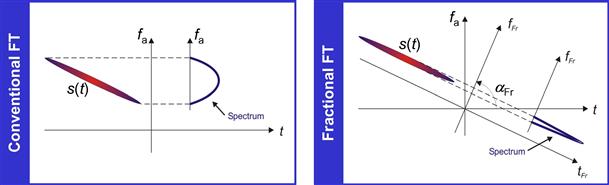
Figure 18.37 Comparison between conventional Fourier transform (left) and Fractional Fourier transform (right) for a LFM signal s(t).
The application of the FrFT for estimating the Doppler slope ![]() is quite similar to the matched filter bank approach. Instead of applying different matched filters for focusing now the FrFT is applied successively on the extracted range compressed data whereby each time a different rotation angle
is quite similar to the matched filter bank approach. Instead of applying different matched filters for focusing now the FrFT is applied successively on the extracted range compressed data whereby each time a different rotation angle ![]() is used. The rotation angle corresponds to the Doppler slope in the following way [35]:
is used. The rotation angle corresponds to the Doppler slope in the following way [35]:
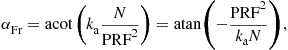 (18.111)
where the ratio between the number of samples N and the PRF is used for normalization purposes. The estimate of the Doppler slope ![]() is then computed with this equation using the optimum rotation angle
is then computed with this equation using the optimum rotation angle ![]() which maximizes the peak amplitude of the spectrum.
which maximizes the peak amplitude of the spectrum.
As with the matched filter bank also the FrFT can cope with multi-component LFM signals as shown in Figure 18.38. On the top the “Fractional Spectra Map” is depicted. This map is obtained by successive application of the fractional Fourier transform with different rotation angles. At the bottom for each of the three moving target signals the spectrum obtained by using the optimum rotation angle is shown.
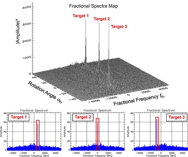
Figure 18.38 Fractional spectra map (top) containing three simulated moving target signals with different Doppler slopes embedded in white Gaussian noise. At the bottom the cuts along the optimum rotation angle ![]() for each of the signals are shown.
for each of the signals are shown.
In contrast to the matched filter bank the application of the FrFT has higher computational cost but also some advantages. For instance, bandpass filtering can be applied directly in the fractional Fourier domain as depicted in Figure 18.39. By this orthogonal interferences can be filtered out and multi-component LFM signals can be separated from each other and extracted from the data. After applying the inverse FrFT on the bandpass filtered signal using -![]() as rotation angle, the clutter and noise suppressed moving target signal is obtained in the time domain.
as rotation angle, the clutter and noise suppressed moving target signal is obtained in the time domain.
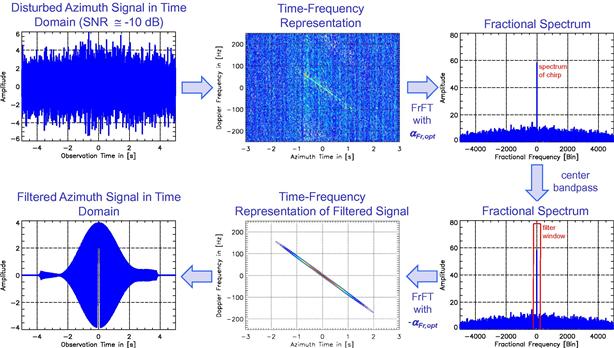
2.18.7.3 Time-frequency analysis
One application of time-frequency (TF) analysis in the field of GMTI is the estimation of the instantaneous Doppler frequency ![]() of the moving target signal. From the estimated instantaneous Doppler frequency (cf. (18.18)) the phase history
of the moving target signal. From the estimated instantaneous Doppler frequency (cf. (18.18)) the phase history ![]() of the range compressed moving target signal can be computed by integration [63]:
of the range compressed moving target signal can be computed by integration [63]:
![]() (18.112)
(18.112)
where ![]() is an unimportant constant phase term. With the estimated phase a proper reference function
is an unimportant constant phase term. With the estimated phase a proper reference function ![]() can be constructed. With this reference function even targets in non-linear motion can be properly focused. Thus, the application of the reference function can already be considered as a simplified ISAR imaging method.
can be constructed. With this reference function even targets in non-linear motion can be properly focused. Thus, the application of the reference function can already be considered as a simplified ISAR imaging method.
Before the phase history can be computed with (18.112) it is necessary to estimate the Doppler frequency ![]() . For this purpose a suitable TF transform has to be applied on the range compressed moving target signal. Probably the best known linear TF transform is the short-time Fourier transform. As disadvantage a trade-off between time and frequency resolution has to be made: either a small time or a small frequency resolution can be obtained. It is impossible to get both simultaneously. In contrast the Wigner-Ville distribution (WVD) is the TF distribution having the best time-frequency resolution [64,65]. However, since it is a quadratic TF transform cross-terms and interferences may occur if the WVD is applied on multi-component LFM signals. To avoid these issues or to keep at least the negative influences at a low level, clutter suppression and signal separation has to be performed prior to its use, e.g., by applying DPCA and range history tracking. In [17] it is shown how the Pseudo Wigner-Ville Distribution (PWVD) can be used for Doppler parameter estimation and ISAR imaging.
. For this purpose a suitable TF transform has to be applied on the range compressed moving target signal. Probably the best known linear TF transform is the short-time Fourier transform. As disadvantage a trade-off between time and frequency resolution has to be made: either a small time or a small frequency resolution can be obtained. It is impossible to get both simultaneously. In contrast the Wigner-Ville distribution (WVD) is the TF distribution having the best time-frequency resolution [64,65]. However, since it is a quadratic TF transform cross-terms and interferences may occur if the WVD is applied on multi-component LFM signals. To avoid these issues or to keep at least the negative influences at a low level, clutter suppression and signal separation has to be performed prior to its use, e.g., by applying DPCA and range history tracking. In [17] it is shown how the Pseudo Wigner-Ville Distribution (PWVD) can be used for Doppler parameter estimation and ISAR imaging.
In Figure 18.40 an example is shown where the PWVD is used for estimating the Doppler slope ![]() of the moving target signal. The PWVD was applied on the same data set used in Section 2.18.7.1 for the explanation of the matched filter bank principle.
of the moving target signal. The PWVD was applied on the same data set used in Section 2.18.7.1 for the explanation of the matched filter bank principle.
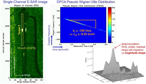
2.18.7.4 Radon transform
Also the Radon transform [60] applied on the TF representation (i.e., the Wigner-Ville spectrum) of the moving target signal can be used for target detection and Doppler slope estimation [66]. An example is shown in Figure 18.41. However, nowadays algorithms relying on the Radon transform of the Wigner-Ville spectrum are replaced increasingly by algorithms using the fractional Fourier transform.
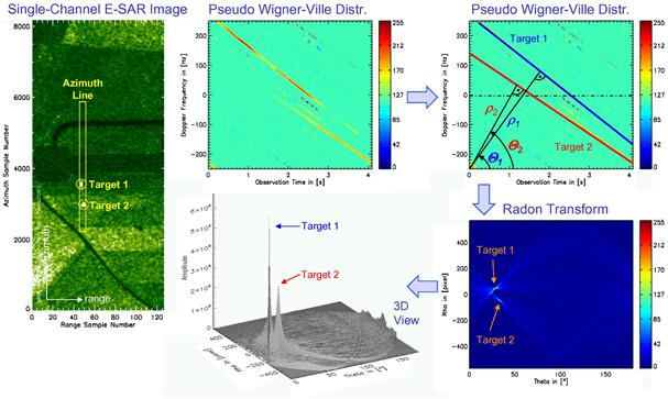
2.18.8 Space-time adaptive processing
The intention of this section is to provide a short introduction to space-time adaptive processing (STAP). A comprehensive tutorial is given in the STAP chapter of the ELSEVIER e-reference. Further reading can be found in [4,37,43,67].
STAP is a two-dimensional filtering technique. It operates in the angle-Doppler plain sketched exemplarily in Figure 18.42. The clutter suppression is performed by beamformers that take into account the space-time nature of the received signals. With the beamforms nulls in the angle-Doppler beampattern can be placed. Doppler histories and angular directions of moving target signals are no longer rigidly coupled. The optimum beamformer or weight vector, respectively, is given in (18.90) in Section 2.18.6.2.2. The difference to adaptive clutter suppression treated in Section 2.18.6.2.2 is that the steering vector ![]() can be adapted to certain signal properties for parameter estimation purposes. However, most of the state-of-the-art STAP algorithms only estimate the line-of-sight velocity
can be adapted to certain signal properties for parameter estimation purposes. However, most of the state-of-the-art STAP algorithms only estimate the line-of-sight velocity ![]() (related to the Doppler shift
(related to the Doppler shift ![]() ) and the direction-of-arrival angle
) and the direction-of-arrival angle ![]() , from which the true target position can be computed. The target’s along-track velocity
, from which the true target position can be computed. The target’s along-track velocity ![]() is not estimated.
is not estimated.
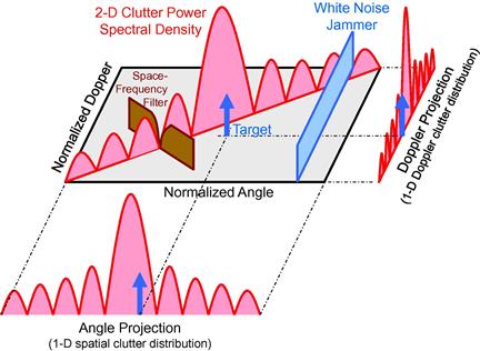
2.18.8.1 Joint domain STAP
Originally STAP was designed to operate in the time domain (note that the data must not be co-registered). STAP processing operates on the radar data cube depicted on the right in Figure 18.43. The data cube is convenient for visualizing subsequent space-time processing although the radar processer does not store the data in the format shown in the figure [68]. Each data cube corresponds to a single coherent processing interval (CPI).
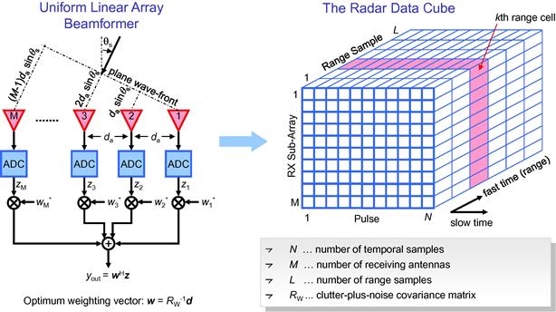
The page of the data cube corresponding to the kth range cell is
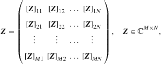 (18.113)
where M is the number of RX channels and N is the number of temporal samples per RX channel. The matrix in previous equation can be vectorized by stacking each succeeding column one beneath the other. This yields the space-time snapshot for the kth range cell, i.e.,
![]() (18.114)
(18.114)
where the elements ![]() are abbreviated as
are abbreviated as ![]() . The space-time snapshot in general is composed of
. The space-time snapshot in general is composed of
![]() (18.115)
(18.115)
where s denotes the moving target signal, c the clutter and n the uncorrelated component due to thermal receiver noise or sky noise. The multi-channel signal for STAP often is modeled as [8]
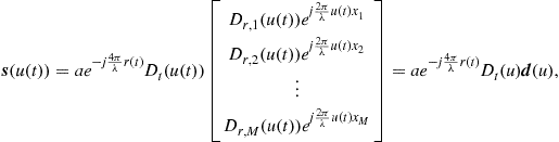 (18.116)
where ![]() is a complex amplitude describing the reflectivity of the scatterer,
is a complex amplitude describing the reflectivity of the scatterer, ![]() denotes the range to the antenna array center,
denotes the range to the antenna array center, ![]() and
and ![]() are the transmit and receive antenna characteristics of the mth channel,
are the transmit and receive antenna characteristics of the mth channel, ![]() and denotes the antenna phase center positions in azimuth direction with respect to the array origin, and
and denotes the antenna phase center positions in azimuth direction with respect to the array origin, and ![]() is the directional cosine. It is assumed that the antenna array center origin is freely chosen at the center of the array, so that
is the directional cosine. It is assumed that the antenna array center origin is freely chosen at the center of the array, so that ![]() . The common phase multiplier
. The common phase multiplier ![]() represents the conventional azimuth chirp used for classical SAR imaging via azimuth compression or matched filtering.
represents the conventional azimuth chirp used for classical SAR imaging via azimuth compression or matched filtering.
The space-time processor linearly combines the elements of the space-time snapshot by applying a weight vector. As result at the output of the space-time processor a scalar is obtained
![]() (18.117)
(18.117)
where H denotes conjugate transposition and w is the complex weight vector of dimension ![]() . The optimal weight vector maximizes the output SCNR and takes, under the assumption of homogeneous Gaussian clutter, the form
. The optimal weight vector maximizes the output SCNR and takes, under the assumption of homogeneous Gaussian clutter, the form
![]() (18.118)
(18.118)
where ![]() is the interference covariance matrix of dimension
is the interference covariance matrix of dimension ![]() and
and ![]() is the steering vector of dimension
is the steering vector of dimension ![]() .
.
In practice both ![]() and d are unknown and need to be estimated. Thus, instead of (18.118) an estimate of the weight vector in the form of
and d are unknown and need to be estimated. Thus, instead of (18.118) an estimate of the weight vector in the form of
![]() (18.119)
(18.119)
is applied, where ![]() is an estimate of
is an estimate of ![]() and v is a surrogate for d. This approach is known as sample matrix inversion (SMI). It is common to compute the covariance matrix estimate as
and v is a surrogate for d. This approach is known as sample matrix inversion (SMI). It is common to compute the covariance matrix estimate as
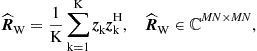 (18.120)
where ![]() of dimension
of dimension ![]() are known as secondary training data. Conventionally K data ranges are used for training (i.e., the averaging is performed along range). To avoid target self-whitening the cell under test as well as cells where already a target has been detected should be excluded from the data.
are known as secondary training data. Conventionally K data ranges are used for training (i.e., the averaging is performed along range). To avoid target self-whitening the cell under test as well as cells where already a target has been detected should be excluded from the data.
2.18.8.2 Post-doppler STAP
Since the classical STAP is computationally inefficient and additionally requires a large number of training cells, STAP algorithms needing lower computational power and less training cells have been developed.
With a linear transformation the space-time snapshot z can be projected into a lower dimensional subspace (= Reduced-Dimension STAP) [68]:
![]() (18.121)
(18.121)
where T is the transformation matrix, ![]() has dimension
has dimension ![]() with
with ![]() . The transformation matrix
. The transformation matrix ![]() is independent of the data. In contrast to the joint-domain STAP the computational burden for matrix inversion drops from
is independent of the data. In contrast to the joint-domain STAP the computational burden for matrix inversion drops from ![]() to
to ![]() . The transformation of the steering vector and the optimal weight vector are given as
. The transformation of the steering vector and the optimal weight vector are given as ![]() and
and ![]() , respectively. The estimate of the covariance matrix again can be computed in the same manner as before, but now using the transformed data
, respectively. The estimate of the covariance matrix again can be computed in the same manner as before, but now using the transformed data ![]() instead of z. The adaptive weight vector using the estimated covariance matrix and a surrogate of the steering vector is given as
instead of z. The adaptive weight vector using the estimated covariance matrix and a surrogate of the steering vector is given as ![]() .
.
A practically implementable and efficient Reduced-Dimension STAP algorithm is Post-Doppler STAP [4]. The space-time snapshot given in (18.114) is transformed to Doppler domain before STAP processing takes place. For the period where target and clutter remain in the same range-Doppler resolution cell, the measured space-time snapshot can be expressed by the random vector [4,8]
![]() (18.122)
(18.122)
where a is a complex constant comprising the target’s RCS among others and ![]() is the clutter-plus-noise interference.
is the clutter-plus-noise interference.
The optimum detection for one range-Doppler resolution cell, under the assumption of homogeneous Gaussian clutter, is achieved by comparing [4]
![]() (18.123)
(18.123)
to a threshold. Clutter suppression is performed by multiplying each Doppler frequency bin ![]() of the signal vector z (i.e., the space-time snapshot transformed to Doppler domain) with the inverse of the clutter-plus-noise covariance matrix
of the signal vector z (i.e., the space-time snapshot transformed to Doppler domain) with the inverse of the clutter-plus-noise covariance matrix ![]() . A target match (i.e., matched filtering) is performed afterwards by multiplying the intermediate result with the complex conjugated and transposed steering vector
. A target match (i.e., matched filtering) is performed afterwards by multiplying the intermediate result with the complex conjugated and transposed steering vector ![]() (i.e., the expected moving target signal). With this matched filtering operation the Doppler shift
(i.e., the expected moving target signal). With this matched filtering operation the Doppler shift ![]() (which is proportional to the line-of-sight velocity
(which is proportional to the line-of-sight velocity ![]() , cf. (18.31)) and the direction-of-arrival angle
, cf. (18.31)) and the direction-of-arrival angle ![]() of the moving target signal (from which the true azimuth position can be computed).
of the moving target signal (from which the true azimuth position can be computed).
The clutter covariance matrix for each Doppler frequency bin can be estimated from the data by performing averaging in range:
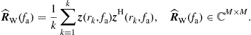 (18.124)
The resulting detection performance in the optimum case is directly proportional to the remaining output SCNR of the optimum filter given as
![]() (18.125)
(18.125)
It can be used for analyzing the detection performance of a given system design [4,8]. Maximizing the SCNR results in a maximized probability of detection ![]() for a fixed false alarm rate
for a fixed false alarm rate ![]() .
.
A visualization example of the SCNR is given in Figure 18.44. Here ![]() and
and ![]() are substituted by the direction-of-arrival angle
are substituted by the direction-of-arrival angle ![]() and the Doppler shift
and the Doppler shift ![]() .
.
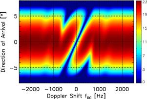
Under assumption of homogeneous Gaussian clutter and non-fluctuating target RCS (Swerling-0 case) the probability of detection can be computed analytically as [68]
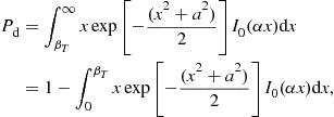 (18.126)
where ![]() is the modified zero-order Bessel function of the first kind and
is the modified zero-order Bessel function of the first kind and ![]() is given as
is given as
![]() (18.127)
(18.127)
The normalized detection threshold ![]() calculates to
calculates to
![]() (18.128)
(18.128)
where ![]() is the desired false alarm rate.
is the desired false alarm rate.
The probability of detection for a given false alarm rate can either be plotted as a function of SCNR, or, more relevant in the field of GMTI, as a function of line-of-sight velocity. An example is shown in Figure 18.45. The minimum detectable velocity (MDV) can directly be read off. For achieving a probability of detection of 0.9 for given SNR and CNR values of 20 dB, the MDVs are approx. 1 m/s (![]() 3.6 km/h) and 1.5 m/s (
3.6 km/h) and 1.5 m/s (![]() 5.4 km/h) for false alarm rates of
5.4 km/h) for false alarm rates of ![]() and
and ![]() , respectively.
, respectively.
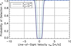
Figure 18.45 Probability of detection for an exemplary system with assumed values of SNR = CNR = 20 dB as a function of line-of-sight velocity for two different false alarm rates.
Most STAP techniques where developed to be used with multi-channel airborne systems. Airborne STAP techniques have in contrast to spaceborne techniques the following advantages:
– High SNR values so that only a small amount of temporal samples has to be considered (at state-of-the art airborne systems 64–256 azimuth samples of each RX channel are used).
– Due to the small amount of samples quadratic and higher order phase terms of the moving target signals can be neglected (but that also implies that the motion parameters normally causing these quadratic and higher order phase terms cannot be estimated with the methods presented in Sections 2.18.6.5 and 2.18.7) so that in most cases a simple FFT is sufficient for focusing without applying a matched filter bank.
– Due to the small amount of samples the range cell migration can be neglected.
The successful application of STAP techniques on multi-channel spaceborne systems is more challenging. Since spaceborne systems suffer from low SNR significantly more temporal samples of the moving target signal need to be integrated coherently for ending up with a sufficient target detection performance. Thus, especially for systems with high range resolution, the range cell migration of the target signal has to be taken into account (cf. Section 2.18.4.1) and a matched filter bank has to be applied (cf. Section 2.18.7.1). Promising novel techniques are the ISTAP (imaging STAP) and EDPCA (extended DPCA) techniques introduced recently in [39,40].
2.18.8.3 EDPCA
The Extended Displaced Phase Center Antenna Technique (EDPCA) is an extension of the DPCA and ATI methods to three or more channels [39,40]. The flow chart of the algorithm is shown in Figure 18.46. The SAR compression filter is matched to the moving target parameters for maximizing target’s SNR. For this task, the application of a bank of SAR processing filters is necessary. That means that for each of the M complex SAR images several times an adapted range cell migration correction and azimuth compression has to be performed. The number of necessary iterations depends on the range resolution and the accepted loss in SCNR compared to the optimum case.
The clutter cancellation filter is either derived from the estimated clutter-plus-noise covariance matrix or pre-computed using the known system, instrument and geometry parameters. EDPCA is partially adaptive and can be used with an arbitrary number of RX channels.
The empirical clutter-plus-noise covariance matrix is estimated by averaging the measured data vector over ![]() range cells and
range cells and ![]() azimuth cells (note that EDPCA operates in contrast to Post-Doppler STAP on fully compressed data) [69]
azimuth cells (note that EDPCA operates in contrast to Post-Doppler STAP on fully compressed data) [69]
 (18.129)
where in the parameter vector ![]() all moving target parameters (i.e., along-track, across-track or line-of-sight velocity) used for adapted SAR are condensed. The clutter-plus-noise covariance matrix is only of dimension
all moving target parameters (i.e., along-track, across-track or line-of-sight velocity) used for adapted SAR are condensed. The clutter-plus-noise covariance matrix is only of dimension ![]() (
(![]() number of RX channels) and is thus invertible with low computational power (
number of RX channels) and is thus invertible with low computational power (![]() ).
).
For achieving a good performance the clutter-plus-noise covariance matrix should be estimated for each image pixel under test. A large number of range and azimuth cells should be used for averaging. The pixel under test and a guard zone should be excluded from training. Already detected targets should also be excluded.
The normalized test statistics is given as [69]
 (18.130)
where ![]() is the steering vector and
is the steering vector and ![]() is a CFAR threshold.
is a CFAR threshold.
What is not shown in the flow chart in Figure 18.46 is a clustering stage, where several pixel-based detections of the same target are clustered to only one physical target.
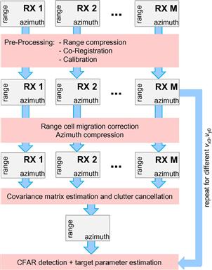
2.18.8.4 ISTAP
Imaging space-time adaptive processing (ISTAP) is a combination of Post-Doppler STAP and SAR [39,40]. As with Post-Doppler STAP clutter cancellation is performed in the Doppler domain. However, there is no segmentation into short coherent processing intervals so that all the data are coherently processed. Thus, high SCNR values can be achieved so that the ISTAP technique is well suited for spaceborne systems.
The flow chart of ISTAP is shown in Figure 18.47. As with EDPCA the SAR compression filter is matched to the moving target parameters for maximizing the target SNR. Again a bank of SAR processing filters is necessary. However, ISTAP requires less computational power since the clutter-plus-noise covariance needs only to be estimated once and not for every iteration. Furthermore, also clutter cancellation needs to be performed only once.
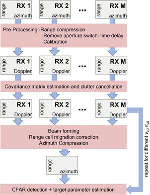
The empirical Doppler-dependent clutter-plus-noise covariance matrix is estimated by averaging the measured data vector over ![]() range cells, identical to conventional Post-Doppler STAP [70]:
range cells, identical to conventional Post-Doppler STAP [70]:
 (18.131)
Again, the clutter-plus-noise covariance matrix is only of dimension ![]() and is thus invertible with low computational power (
and is thus invertible with low computational power (![]() ).
).
The clutter-plus-noise covariance matrix needs to be estimated for each Doppler bin.
The normalized test statistics for ISTAP is given as [70]
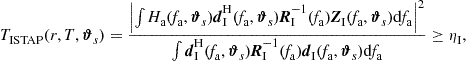 (18.132)
where ![]() is the SAR transfer function (only the Doppler slope is considered but not the shift) which maximizes the SNR of the target with parameter
is the SAR transfer function (only the Doppler slope is considered but not the shift) which maximizes the SNR of the target with parameter ![]() is the steering vector and
is the steering vector and ![]() is the CFAR threshold.
is the CFAR threshold.
2.18.9 Conclusion and future trends
A tutorial for GMTI with multi-channel SAR systems was provided. The SAR principle was explained and a single- and multi-channel moving point target signal model was derived. A special focus was laid on the effects caused by moving target signals in the SAR images. The knowledge about these effects is essential for understanding the different parameter estimation methods. The classical dual-channel techniques ATI and DPCA and their limitations were discussed in detail, since they are currently of special importance for state-of-the-art spaceborne SAR-GMTI systems. A general GMTI processing chain was presented and basic Doppler parameter estimation methods were introduced. Also a short introduction to STAP, which is covered in detail by a separate chapter in the ELSEVIER e-reference, was given.
The ongoing research in GMTI can be summarized as:
• Improvement of the target detection performance and the reduction of false alarms.
• Accurate and robust SAR-GMTI algorithms for spaceborne SAR-MTI systems.
• Improvement of the position and motion parameter estimation performance. This is of special importance for spaceborne SAR-GMTI where due to low SNR and SCNR values large estimation errors may arise. First promising techniques are ISTAP and EDPCA introduced in [39,40]. A different method requiring a large along-track baseline was presented in [71].
• Reduction of the system complexity and processing time. This is of special importance for affordable real-time systems to be used for civilian traffic monitoring. A suitable technique which also can be combined with classical STAP was introduced in [72].
• Trend to shorter wavelengths (e.g., Ka-band with wavelengths in the order of 8 mm): this allows for smaller instruments enabling both high resolution and good GMTI performance.
• Low PRF GMTI algorithms which can be used together with high-resolution wide swath (HRWS) SAR imaging.
2.18.9.1 Summary of algorithms
In Table 18.2 a summary of the algorithms treated in this tutorial is given. Also the parameter estimation accuracy and the required computational load are assessed in a qualitative way.

Applications:
Open Issues and Problems:
– Accurate estimation of moving target’s along-track velocity, especially without the negative influence of accelerations.
– Improvement of the moving target parameter estimation accuracy of spaceborne GMTI algorithms.
Glossary
ATI along-track interferometry; the phase differences of the signals received by two antennas separated in along-track or flight direction are measured. The phase difference is related to moving target parameters.
Clutter unwanted radar echos; for GMTI echos from the stationary background scene are considered as clutter
DPCA displaced phase center antenna; similar antenna arrangement as with ATI but instead of the phases the amplitudes are evaluated. Commonly DPCA is used for suppressing the clutter, i.e., the signals of stationary targets.
IRF impulse response function; focused signal of a point target
(G)MTI (ground) moving target indication; the detection of targets moving on ground and the estimation of their geographical positions, their velocities and moving directions.
SAR synthetic aperture radar; a side-looking imaging radar system exploiting the Doppler effect due to platform motion for imaging
SCNR signal-to-clutter-plus-noise ratio
STAP space-time adaptive processing
SWMF stationary world matched filter; a two-dimensional filter used for SAR processing; every conventional SAR processor is considered as a SWMF in this tutorial
Relevant Theory: Signal Processing Theory and Array Signal Processing
See Vol. 1, Chapter 3 Discrete-Time Signals and Systems
See Vol. 1, Chapter 12 Adaptive Filters
See Vol. 3, Chapter 19 Array Processing in the Face of Nonidealities
References
1. Tomiyasu K. Tutorial review of synthetic-aperture radar SAR with applications to imaging of the ocean surface. Proc IEEE. 1978;66:563–583.
2. Skolnik MI, ed. Radar Handbook. second ed. McGraw-Hill 1990.
3. Cumming IG, Wong FH. Digital Signal Processing of Synthetic Aperture Radar: Algorithms and Implementation. Artech House 2005.
4. Ender JHG. Space-time processing for multichannel synthetic aperture radar. Electron Commun Eng J. 1999;11:29–38.
5. Raney RK. Synthetic aperture imaging radar and moving targets. IEEE Trans Aerosp Electro Syst. 1971;AES-7(3):499–505.
6. Werninghaus R, Buckreuss S. The terraSAR-X mission and system design. IEEE Trans Geosci Remote Sens. 2010;48(2):606–614.
7. Ender JHG. The airborne experimental multi-channel SAR system AER-II. In: 1st European Conference on Synthetic Aperture Radar (EUSAR), Königswinter, Germany. March 1996;49–52.
8. Ender JHG, Gierull CH, Cerutti-Maori D. Improved space-based moving target indication via alternate transmission and receiver switching. IEEE Trans Geosci Remote Sens. 2008;46(12):3960–3974.
9. Bethke K, Baumgartner S, Gabele M, et al. Air-and spaceborne monitoring of road traffic using SAR moving target indication—Project TRAMRAD. ISPRS J Photogramm Remote Sens. 2006;61(3–4):243–259.
10. Cerutti-Maori D, Klare J, Brenner AR, Ender JGH. Wide area traffic monitoring with the SAR/GMTI system PAMIR. Trans Geosci Remote Sens. 2008;46(10):3019–3030.
11. Suchandt S, Runge H, Breit H, Steinbrecher U, Kotenkov A, Balss U. Automatic extraction of traffic flows using terraSAR-X along-track interferometry. IEEE Trans Geosci Remote Sens. 2010;48(2):807–819.
12. Baumgartner SV, Krieger G. Real-time road traffic monitoring using a fast a priori knowledge based SAR-GMTI Algorithm. In: IEEE International Geoscience and Remote Sensing Symposium (IGARSS). Hawaii, USA: Honolulu; July 2010.
13. (2012, March) Floating car data. <http://en.wikipedia.org/wiki/Floating_car_data>.
14. Koch W, Klemm R. Ground target tracking with stap radar. IEE Proc -Radar Sonar Navig. 2001;148(3):173–185.
15. Chen V, Ling H. Time-Frequency Transforms for Radar Imaging and Signal Analysis. Artech House Publishers 2002.
16. Berens P, Gebhardt U, Holzner J. ISAR imaging of ground moving vehicles using PAMIR data. In: International Radar Conference—Surveillance for a Safer World (RADAR), Bordeaux, France. October 2009;1–5.
17. W. Rieck, Zeit-Frequenz-Signal-Analyse für Radaranwendungen mit synthetischer Apertur (SAR), Ph.D. Dissertation, Rheinisch-Westfälische Technische Hochschule Aachen, 1997.
18. Chiu S, Dragosevic MV. Moving target indication via RADARSAT-2 multichannel synthetic aperture radar. EURASIP J Adv Signal Process. 2010;2010.
19. Curlander JC, McDonough RN. Synthetic Aperture Radar: Systems and Signal Processing. Wiley-Interscience 1991.
20. Moreira A, Mittermayer J, Scheiber R. Extended chirp scaling algorithm for air- and spaceborne SAR data processing in stripmap and scanSAR imaging modes. IEEE Trans Geosci Remote Sens. 1996;34(5):1123–1136.
21. J.J. Sharma, The Influence of Target Acceleration on Dual-Channel SAR-GMTI (Synthetic Aperture Radar Ground Moving Target Indication) Data, University of Calgary, Calgary, Alberta, Canada, Master Thesis, October 2004.
22. Sharma JJ, Gierull CH, Collins MJ. Compensating the effects of target acceleration in dual-channel SAR-GMTI. IEE Proc Radar Sonar Navig. 2006;153(1):53–62.
23. Sharma JJ. The influence of target acceleration on velocity estimation in dual-channel SAR-GMTI. IEEE Trans Geosci Remote Sens. 2006;44(1):134–147.
24. Baumgartner S, Krieger G. Acceleration-independent along-track velocity estimation of moving targets. IET Radar Sonar Navig. 2010;4(3):474–487.
25. Perry RP, DiPietro RC, Fante RL. SAR imaging of moving targets. IEEE Aerosp Electron Syst. 1999;35(1):188–200.
26. Jao J. Theory of synthetic aperture radar imaging of a moving target. IEEE Trans Geosci Remote Sens. 2001;39(9):1984–1992.
27. Meyer F, Hinz S, Laika A, Bamler R. A-priori information driven detection of moving objects for traffic monitoring by sar. In: 2005;2932–2936. Proc IEEE Int Geosci Remote Sens Symp IGARSS ’05. vol. 4.
28. Goldstein RM, Zebker HA. Interferometric radar measurements of ocean surface currents. Nature. 1987;328:707–709.
29. Zebker HA, Villasenor J. Decorrelation in interferometric radar echoes. IEEE Trans Geosci Remote Sens. 1992;30(5):950–959.
30. Rodriguez E, Martin JM. Theory and design of interferometric synthetic aperture radars. IEE Proc F Radar Signal Process. 1992;139(2):147–159.
31. Just D, Bamler R. Phase statistics of interferograms with applications to synthetic aperture radar. Appl Optics. 1994;33(20):4361–4368.
32. Budillon A, Ferraiuolo G, Pascazio V, Schirinzi G. EURASIP J Appl Signal Process. EURASIP J Appl Signal Process. 2005;2005(20):3180–3193.
33. Budillon A, Pascazio V, Schirinzi G. Estimation of radial velocity of moving targets by along-track interferometric sar systems. IEEE Geosci Remote Sens Lett. 2008;5(3):349–353.
34. Gierull CH. Statistical analysis of multilook SAR interferograms for CFAR detection of ground moving targets. IEEE Trans Geosci Remote Sens. 2004;42(4):691–701.
35. Chiu S. Application of fractional fourier transform to moving target indication via along-track interferometry. EURASIP J Appl Signal Process. 2005;20:3293–3303.
36. F.R. Dickey, M.M. Sante, Final report on anti-clutter techniques, General Electric Co., Heavy Military Electron. Dept., Syracuse, NY, Rep. No. R65EMH37, 1953.
37. Klemm R. Space-Time Adaptive Processing: Principles and Applications. UK: IEE; 1998.
38. Lombardo P, Colone F, Pastina D. Monitoring and surveillance potentialities obtained by splitting the antenna of the COSMO-SkyMed SAR into multiple sub-apertures. IEE Proc Radar Sonar Navig. 2006;153(2):104–116.
39. Cerutti-Maori D, Sikaneta I. Optimum GMTI processing for space-based SAR/GMTI systems—theoretical deviation. In: European Conference on Synthetic Aperture Radar (EUSAR), Aachen, Germany. June 2010;1–4.
40. Cerutti-Maori D, Sikaneta I. Optimum GMTI processing for space-based SAR/GMTI systems—simulation results. In: European Conference on Synthetic Aperture Radar (EUSAR), Aachen, Germany. June 2010;1–4.
41. C.H. Gierull, Digital Channel Balancing of Along-Track Interferometric SAR Data, Defence R&D Canada, Ottawa, Canada, Technical Memorandum DRDC Ottawa TM 2003–024, March 2003.
42. Chiu S, Gierull C, Durak A. Clutter effects on ground moving targets’ interferometric phase. In: July 2005;2928–2931. IEEE Geoscience and Remote Sensing Symposium (IGARSS). vol. 4 Seoul, Korea.
43. Guerci JR. Space-Time Adaptive Processing for Radar. Artech House 2003.
44. Banahan CP, Perks D, Baker C, Woodbridge K. GMTI clutter cancellation using real non-ideal data. IET Radar Sonar Navig. 2010;4(2):302–314.
45. Sikaneta IC, Chouinard J-Y. Eigendecomposition of the multi-channel covariance matrix with applications to SAR-GMTI. Signal Process. 2004;84(9):1501–1535.
46. C.H. Gierull, Moving Target Detection with Along-Track SAR Interferometry, Defence RD Canada–Ottawa, Tech. Rep. DRDC Ottawa TR 2002–084, August 2002.
47. Gierull CH, Sikaneta IC. Raw data based two-aperture SAR ground moving target indication. In: July 2003;1032–1034. IEEE Internation Geoscience and Remote Sensing Symposium (IGARSS), Toulouse, France. vol. 2.
48. Baumgartner SV, Krieger G. SAR traffic monitoring using time-frequency analysis for detection and parameter estimation. In: USA: Boston; July 2008;II-25–II-28. IEEE International Geoscience and Remote Sensing Symposium (IGARSS). vol. 2.
49. Baumgartner SV, Gabele M, Krieger G, Bethke K-H, Zuev S. Traffic monitoring with SAR: implications of target acceleration. In: 6th European Conference on Synthetic Aperture Radar (EUSAR), Dresden, Germany. May 2006.
50. Zhou F, Wu R, Xing M, Bao Z. Approach for single channel SAR ground moving target imaging and motion parameter estimation. IET Radar Sonar Navig. 2007;1(1):59–66.
51. Gierull CH. Azimuth positioning of moving targets in two-channel SAR by direction-of-arrival estimation. Electron Lett. 2004;40(21):1380–1381.
52. Meyer F, Hinz S, Laika A, Weihing D, Bamler R. Performance analysis of the TerraSAR-X traffic monitoring concept. ISPRS J Photogramm Remote Sens. 2006;61(3–4):225–242.
53. Baumgartner S, Krieger G. Acceleration independent along-track velocity estimation of moving targets. In: June, 2008;207–210. 7th European Conference on Synthetic Aperture Radar (EUSAR), Friedrichshafen, Germany. vol. 4.
54. Automatic Identification System, June 2011. <http://en.wikipedia.org/wiki/Automatic_Identification_System>.
55. Baumgartner SV, Krieger G. Large along-track baseline SAR-GMTI: first results with the TerraSAR-X/TanDEM-X satellite constellation. In: Proceedings of the IEEE International Geoscience and Remote Sensing Symposium (IGARSS), Vancouver, Canada. July 2011;1319–1322.
56. Barbarossa S. Detection and imaging of moving objects with synthetic aperture radar -Part 1: Optimal detection and parameter estimation theory. IEE Proc. 1992;F 139(1):79–88.
57. Gabele M, Sikaneta I. Motion parameter estimation of Doppler-Ambiguous moving targets in SAR-GMTI. In: International Radar Symposium (IRS). Germany: Cologne; September 2007.
58. Scheiber R, Prats P, Nannini M, et al. Advances in airborne SAR interferometry using the experimental SAR system of DLR. In: European Microwave Week (EuMW). Munich, Germany: Horizon House; October 2007;91–94.
59. Almeida LB. The fractional Fourier transform and time-frequency representations. IEEE Trans Signal Process. 1994;42(11):3084–3091.
60. Radon J. Über die Bestimmung von Funktionen durch ihre Integralwerte längs gewisser Mannigfaltigkeiten, Berichte Sächsische Akademie der Wissenschaften, Leipzig. Mathematisch-Physikalische Klasse. 1917;69:262–277.
61. Kutay A, Ozaktas H, Ankan O, Onural L. Optimal filtering in fractional Fourier domains. IEEE Trans Signal Process. 1997;45(5):1129–1143.
62. Sun H-B, Liu GS, Gu H, Su W-M. Application of the fractional Fourier Transform to moving target detection in airborne SAR. IEEE Trans Aerosp Electron Syst. 2002;38(4):1416–1424.
63. Barbarossa S, Farina A. Detection and imaging of moving objects with synthetic aperture radar 2 Joint time-frequency analysis by Wigner-Ville distribution. IEE Proc F. 1992;139(1):89–97.
64. Claasen TACM, Mecklenbräuker WFG. The Wigner distributiona tool for time-frequency signal analysis, Part I: Continuous-time signals. Philips J Res. 1980;35(3):217–250.
65. Claasen TACM, Mecklenbräuker WFG. The Wigner distributiona tool for time-frequency signal analysis, Part II: Discrete time signals. Philips J Res. 1980;35(4–5):276–300.
66. Wood JC, Barry DT. Radon transformation of time-frequency distributions for analysis of multicomponent signals. IEEE Trans Signal Process. 1994;42(11):3166–3177.
67. Barbarossa S, Farina A. Space-time-frequency processing of synthetic aperture radar signals. IEEE Trans Aerosp Electron Syst. 1994;30(2):341–358.
68. Melvin WL. A STAP overview. IEEE A&E Syst Mag. 2004;19(1):19–35.
69. Cerutti-Maori D, Sikaneta I. A generalization of DPCA processing for multi-channel SAR/GMTI radars. IEEE Trans Geosci Remote Sens. 2013;51(1):560–572.
70. Cerutti-Maori D, Sikaneta I, Gierull CH. Optimum SAR/GMTI processing and its application to the radar satellite RADARSAT-2 for traffic monitoring. IEEE Trans Geosci Remote Sens. 2012;(50 10):3868–3881.
71. Baumgartner SV, Krieger G, Bethke K-H. A Large along-track baseline approach for ground moving target indication using TanDEM-X. In: International Radar Symposium (IRS). Germany: Cologne; September 2007.
72. Baumgartner SV, Krieger G. Fast GMTI Algorithm for traffic monitoring based on a priori knowledge. IEEE Trans Geosci Remote Sens. 2012;50(11):4626–4641.
1For interpretation of color in Figure 18.11, the reader is referred to the web version of this book.