
Through-the-Wall Radar Imaging: Theory and Applications
Moeness G. Amin* and Fauzia Ahmad†, *Center for Advanced Communications, Villanova University, Villanova, PA, USA, †Radar Imaging Lab, Center for Advanced Communications, Villanova University, Villanova, PA, USA, [email protected], [email protected]
Abstract
Through-the-Wall radar imaging (TWRI) is emerging as a viable technology for providing high quality imagery of enclosed structures. TWRI makes use of electromagnetic waves below the S-band to penetrate through building wall materials. The indoor scene can be illuminated from each antenna, and be reconstructed using the data from the receive antennas. Due to the “see”-through ability, TWRI has attracted much attention in the last decade with a variety of important civilian and military applications. For instance, this technology is employed for surveillance and detection of humans and interior objects in urban environments, and for search and rescue operations in military situations. In this chapter, we cover signal processing algorithms that proved valuable in allowing proper imaging and image recovery in the presence of high clutter, caused by front walls, and multipath, caused by reflections from internal walls. Specifically, we focus on ground-based imaging systems which are relatively mature, and discuss wall mitigation techniques, multipath exploitation methods, change detection of moving target, and compressive sensing for fast data acquisition.
Keywords
Through-the-wall radar; Urban sensing; Compressive sensing; Multipath exploitation; Clutter mitigation; Moving target indication; Beamforming; Backprojection
2.17.1 Introduction
The field of remote sensing has developed a range of interesting imaging approaches for a variety of applications. Through-the-wall sensing is a relatively new area that addresses the desire to see inside buildings for various purposes, including determining the room layouts, discerning the building intent and nature of activities, locating the occupants, and even identifying and classifying objects within the building. Through-the-wall sensing is highly desired by police, fire and rescue, emergency relief workers, and military operations. Accurate sensing and imaging can allow a police force to obtain an accurate description of a building in a hostage crisis, or allow firefighters to locate people trapped inside a burning structure. In essence, the goals of through-the-wall sensing technology are to provide vision into otherwise obscured areas [1].
Each remote sensing application area has driven different sensing modalities and imaging algorithm development based upon propagation characteristics, sensor positioning, and safety issues. Traditional optical, radar, and sonar image processing all begin with basic wave physics equations to provide focusing to individual points. In many radar applications, for example, data sampled from many sensors are mathematically integrated to provide equivalent focusing using free-space propagation assumptions. Free-space imaging is commonly seen in synthetic aperture radar (SAR) techniques since atmospheric distortions are often negligible and can be safely ignored in first-order calculations [2].
Conventional imaging approaches exploit the wave equation to compute the expected phase at each point in space and time over which the data are collected. The complex phase front is similar to the spatial representation of the wavefront captured by a hologram [3]. The complex returns can then be compared against the predicted returns from points in the imaging target space to focus on each point in that space. The focusing is analogous to image reconstruction in holography, where a spatial pattern is projected back into the originating target image space. In true free-space conditions, this focusing approach represents a mathematically accurate way to perform imaging. More sophisticated approaches extend beyond free-space assumptions to allow for more complicated propagation effects, such as adaptive optics [4], atmospheric correction for radar [2], and matched field processing for sonar [5]. Correction approaches range from simple wavefront calibration to more sophisticated volumetric propagation corrections.
Free-space propagation does not apply to several applications where transmission through scattering media is encountered, including many modern imaging approaches such as geophysical sensing, medical imaging, and more recently through-the-wall imaging and sensing. In these applications, propagating signals diffract through a volume. As examples, geophysical imaging techniques generally measure seismic propagation through the earth to look for discontinuities that are often indicators of oil, gas, water, or mineral deposits [6]. In medical imaging, ultrasound tomographic approaches account for propagation through different tissue classes [7].
Non-freespace scattering applications are more representative of the through-the-wall sensing problem, albeit each has its own distinct challenges and approaches [1]. In geophysical and medical applications, the propagation medium is discontinuous but still respectively fills the sensing volume of the earth and tissue. To better propagate into the volume, sensors are placed in direct contact with the medium (e.g., seismometers for geophysical sensing, ultrasound transducers for medical imaging). In through-the-wall sensing, there are many air-material interfaces that dramatically change the wavefront. Through-the-wall sensors may be placed against the front walls or located some distance away from the structure. In either case, attenuation is largely seen only in the building materials and contents rather than in the large volumes of air that occupy most of the space outside or within a building. The rich through- the-wall scattering environment makes volumetric tomographic imaging approaches most relevant for through-the-wall sensing. Rather than using free-space focusing assumptions, correcting for propagation effects may greatly improve the imaging solution [8–10].
Through-the-wall sensing is best motivated by examining the applications primarily driving its development. Through-the-wall sensing grew from the application of ground-penetrating radar systems to walls, with specific applications documented in the literature since the late 1990s showing abilities to sense beyond a single wall from near range [11–25]. Applications can be divided based upon whether information is sought on motions within a structure or on imaging the structure and its stationary contents.
The need to detect motion is highly desired in situations like firefighters finding a child in a burning building or law enforcement officers locating hostages and their captors. Such applications can resort to Doppler discrimination of movement from background clutter [26–31]. Motion detection and localization can be decomposed into zero (0-D), one (1-D), two (2-D), or three-dimensional (3-D) systems. A 0-D system is simply a motion detector and will report any motion in the scene. Such systems may be useful to detect whether a room is occupied or not, often useful in monitoring applications such as security systems or intruder detection. Interior motion may be ample information for a firefighter to decide whether to enter a room or building. Since range or angle is not required, 0-D systems may use continuous wave (CW) tones as waveforms. While such systems have exquisite sensitivity, it is difficult to confine the sensitivity to desired areas, so care must be taken to prevent undesired detections beyond the intended range or even from the system operator himself due to multipath reflections. 0-D systems are not particularly useful in cases where other moving individuals may be within the sensor field of view.
One-dimensional systems provide a range to a target but not an angle. The extra dimension provides the ability to separate and possibly discriminate multiple targets. The range information can help bound whether a detection is in the adjacent room, or perhaps deeper within the building. The systems can obviously gate out detections from ranges beyond the ranges of interest, and may more easily discriminate desired target motion from the motion of the operator. The systems often consist of a single receiving antenna in addition to a transmitting antenna (although sometimes a single antenna can be used for both functions). Motion of the operator can be gated out in range, or a reference antenna pointed towards the radar operator can be used for cancellation. Ranging is historically one of the principle reasons for the development of radar technology, but the short stand-off ranges of most through-the-wall systems provide some particular challenges. Three methods are often employed to obtain target range, namely, ultrawideband pulses [22,32–36], dual frequencies [28,37–39], or stepped CW [11,20].
Two-dimensional systems provide a slice through the scene in the range and angle dimensions [11,22,23]. The 2-D representation provides better localization of the mover, at the expense of a larger antenna array whose elements are collinear. 2-D systems will be subject to layover of objects, meaning that objects out of plane will appear to be rotated to the imaging plane, which can lead to distortion of the field of view. 3-D systems attempt to represent a volumetric representation of the field of view in the range, azimuth, and elevation dimensions [40]. The third dimension avoids the layover issue of targets being projected into a 2-D plane; at the expense of a 2-D array and higher processing requirements. Potentially, the third dimension can provide additional localization for identification of targets. Height information may allow discrimination between people and animals such as household pets, since radar cross-section alone can be unreliable in the presence of through-the-wall multipath and other issues. The ultimate goal is higher resolution for even better moving target classification. Both 2-D and 3-D processing techniques have generally used either multilateration [8,17] or SAR techniques [41,42] using either ultrawideband pulses or stepped CW radars to localize features in the scene.
Imaging of structural features and contents of buildings requires at least 2-D (and preferably 3-D) systems. It cannot rely on Doppler processing for separation of desired features, so multilateration or SAR approaches have been the most commonly used approaches. The general idea behind multilateration is to correlate range measurements from multiple sensors to specific points in the image. With sufficient spatial diversity from a large set of transmit/receive combinations, specific reflection points will start to integrate above the background interference. However, ambiguities will arise as the number of reflection points increases which can provide an over-determined system relative to the transmit/receive signal pairs which can detract from image quality. SAR-based systems can be thought of as a coherent extension of the multilateration concept. Instead of incoherent combinations of range returns from multiple transmit/receive pairs, coherent algorithms are used to provide a complex matched filter to specific points in the target space. SAR algorithms are well established for stand-off imaging applications [2]. Stand-off applications generally assume free-space propagation to each point in the target scene, although platform motion compensation and atmospheric effects are removed with autofocusing algorithms.
Most of the SAR and multilateration techniques usually neglect propagation distortions such as those encountered by signals passing through walls and objects. Distortions degrade the performance and can lead to ambiguities in target and wall localizations. Free-space assumptions no longer apply after the electromagnetic waves propagate through the first wall. As a result, free-space approximations may carry imaging systems through to the first wall, but propagation effects will then affect further imaging results. Shadowing, attenuation, multipath, reflection, refraction, diffraction, and dispersion, all play a role in how the signals will propagate after the first interface. Without factoring in propagation effects, imaging of contents within buildings will be severely impacted. As such, image formation methods, array processing techniques, target detection, image sharpening, and clutter and multipath identification and rejection paradigms must work in concert and be reexamined in view of the nature and specificities of the underlying sensing problem.
A common occurrence of incorrect localization is objects outside the building being illuminated by the reflection off the first wall and subsequently creating an ambiguous image visible inside the building. Moreover, the strong front wall reflection causes nearby indoor weak targets to go undetected. Multipath propagation introduces ghosts or false targets in the image. Uncompensated refraction through walls can lead to localization or focusing errors, leading to offsets and blurring of imaged targets [41,43–45]. Bragg scattering off repeating structural elements, such as rebar in concrete walls or repetitive voids in concrete block walls, can cause image ambiguities and modulation of subsequent wavefronts. Some of the wall propagation effects can be compensated for using image-focusing techniques incorporating proper wavefront corrections [41,44]. SAR techniques and tomographic algorithms, specifically tailored for through-the-wall imaging, are capable of making some of the adjustments for wave propagation through solid materials. While such approaches are well suited for shadowing, attenuation, and refraction effects, they do not account for multipath, Bragg scattering, as well as strong reflections from the front wall.
In this chapter, we consider the recent algorithmic advances that address some of the aforementioned unique challenges in through-the-wall sensing operations. More specifically, Section 2.17.2 deals with techniques for the mitigation of the wall clutter. Front wall reflections are often stronger than target reflections, and they tend to persist over a long duration of time. Therefore, weak and close by targets behind walls become obscured and invisible in the image. Approaches based on both electromagnetic modeling and signal processing are advocated to significantly mitigate the front wall clutter. Section 2.17.3 presents an approach to exploit the rich indoor multipath environment for improved target detection. It uses a ray tracing model to implement a multipath exploitation algorithm, which maps each multipath ghost to its corresponding true target location. In doing so, the algorithm improves the radar system performance by aiding in ameliorating the false positives in the original SAR image as well as increasing the SNR at the target locations, culminating in enhanced behind the wall target detection and localization. Section 2.17.4 discusses a change detection approach to moving target indication for through-the-wall applications. Change detection is used to mitigate the heavy clutter that is caused by strong reflections from exterior and interior walls. Both coherent and noncoherent change detection techniques are examined and their performance is compared using real data collected in a semi-controlled laboratory environment. Section 2.17.5 deals with fast data acquisition schemes to provide timely actionable intelligence in through-the-wall operations. The demand for high degree of situational awareness to be provided by through-the-wall radar systems requires the use of wideband signals and large antenna arrays. As a result, large amounts of data are generated, which presents challenges in both data acquisition and processing. The emerging field of compressive sensing is employed to provide the means to circumvent possible logistic difficulties in collecting measurements in time and space and provide fast data acquisition and scene reconstruction for moving target indication.
It is noted that the chapter provides a signal processing perspective to through-the-wall radar imaging. Outside the scope of this chapter, there has been significant work performed for TWRI applications in the areas of antenna and system design [36,46–48], wall attenuation and dispersion [49–51], electromagnetic modeling [52–55], inverse scattering approaches [24,56,57], and polarization exploitation [58–60].
The progress reported in this chapter is substantial and noteworthy. However, many challenging scenarios and situations remain unresolved using the current techniques and, as such, further research and development is required. However, with the advent of technology that brings about better hardware and improved system architectures, opportunities for handling more complex building scenarios will definitely increase.
2.17.2 Wall clutter mitigation
Scattering from the exterior front wall is typically stronger than that from targets of interest, such as a human or a rifle, which have relatively small radar cross sections (RCS). This makes imaging of stationary targets behind walls difficult and challenging. The problem is further compounded when targets are in close vicinity of walls of either a high dielectric constant or with layered structures. In particular, hollow cinder block walls contain an air-gap void within the cinder block with disparate dielectric constants. This establishes a periodic structure resonance cavity that traps electromagnetic (EM) modes. The consequence of this layered composite structure on radar target imaging is to introduce long time constant relaxations on target detections in radar range profiles. Therefore, weak and close by targets behind walls become obscured and sometimes totally invisible in the image. Thus, wall reflections should be suppressed, or significantly mitigated, prior to applying image formation methods. One of the simple but effective methods is based on background subtraction. If the received signals can be approximated as the superposition of the wall and the target reflections, then subtracting the raw complex data without target (empty scene) from that with the target would remove the wall contributions and eliminate its potential overwhelming signature in the image. Availability of the empty scene, however, is not possible in many applications, and one must resort to other means to deal with strong and persistent wall reflections.
In the past few years, a number of approaches have been proposed to mitigate the front wall returns and effectively increase the signal-to-clutter ratio. For example, the wall reflections can be gated out, the corresponding parameters can be estimated, and then used to model and subtract the wall contributions from the received data [44]. This wall-dependent technique is effective, but its performance is subject to wall estimation and modeling errors. Another method is proposed in [42], which employs three parallel antenna arrays at different heights. The difference between the received signals at two different arrays is used for imaging. Due to the receiver symmetry with respect to the transmitter, a simple subtraction of the radar returns leads to wall reflection attenuation and image improvement. However, this technique requires two additional arrays and the effect of the subtraction operation on the target reflection is unknown and cannot be controlled. In [54], the walls reflections are eliminated by operating the imaging radar in cross-polarization as the cross-polarization returns from a planar interface such as the wall surface are theoretically zero, unlike the returns from humans. However, the cross-polarization returns from the targets behind walls are often very weak compared to their co-polarization counterparts, and as such, the radar performance may be limited by noise.
An eigen-structure technique is developed in [61] to decompose the received radar signal into three subspaces: clutter (including the front wall), target, and noise. Singular value decomposition (SVD is applied on the data matrix to extract the target signatures. SVD has also been used as a wall clutter reduction method for TWRI in [62,63]. Another approach for wall clutter mitigation is based on spatial filtering. It utilizes the strong similarity between wall EM responses, as viewed by different antennas along the entire physical or synthesized array aperture, is proposed in [64]. The idea is that under monostatic radar operation, the wall returns approximately assume equal values and identical signal characteristics across the array elements, provided that the extent of the wall is much greater than the antenna beamwidth. On the other hand, returns from targets with limited spatial extent, such as humans, vary from sensor to sensor. The dc component corresponding to the constant-type return, which is typical of walls, can be significantly reduced while preserving the target returns by applying an appropriate spatial filter along the array axis. However, care must be exercised in the choice of the spatial filter so that its characteristics cause minimum distortion to the target returns. The spatial-domain preprocessing scheme is analogous, in its objective, to the moving target indication (MTI) clutter filter operation in the time domain.
In this section, we present in details two of the aforementioned methods, namely, the wall parameter estimation method and the spatial filtering technique. For the spatial filtering technique, we consider two different types of filters, namely, moving average subtraction filter and the infinite impulse response notch filter, and compare their effects on the target image.
2.17.2.1 Spatial filtering
2.17.2.1.1 Characteristic of the wall reflection
Assume a synthetic aperture radar (SAR) is used in which a single antenna at one location transmits and receives the radar signal, then moves to the next location, and repeats the same operation along the axis parallel to the wall. Assume N antenna locations. With the wall reflection, the received signal at the ![]() th antenna due to a single point target of complex reflectivity
th antenna due to a single point target of complex reflectivity ![]() is given by
is given by
![]() (17.1)
(17.1)
where ![]() is the signal reflected from the wall,
is the signal reflected from the wall, ![]() is the two-way traveling time of the signal from the nth sensor to the wall,
is the two-way traveling time of the signal from the nth sensor to the wall, ![]() is the transmitted signal convolved with the two-way transmission transfer function of the wall, and
is the transmitted signal convolved with the two-way transmission transfer function of the wall, and ![]() is the two-way traveling time between the
is the two-way traveling time between the ![]() th antenna and the target. Note that
th antenna and the target. Note that ![]() is assumed to be independent of frequency and
is assumed to be independent of frequency and ![]() does not vary with the sensor location since the wall is parallel to the array. Furthermore, if the wall is homogeneous and much larger than the beamwidth of the antenna, the wall reflection
does not vary with the sensor location since the wall is parallel to the array. Furthermore, if the wall is homogeneous and much larger than the beamwidth of the antenna, the wall reflection ![]() will be the same for all antenna locations. This implies that the first term in (17.1) assumes the same value across the array aperture. When the wall is not parallel to the array axis,
will be the same for all antenna locations. This implies that the first term in (17.1) assumes the same value across the array aperture. When the wall is not parallel to the array axis, ![]() should be calculated for each sensor location. Compensations for signal attenuations due to differences in the two-way traveling distances for different antenna positions should be performed prior to filtering.
should be calculated for each sensor location. Compensations for signal attenuations due to differences in the two-way traveling distances for different antenna positions should be performed prior to filtering.
Unlike ![]() , the time delay
, the time delay ![]() in (17.1) changes with each antenna location, since the signal path from the antenna to the target is different. For
in (17.1) changes with each antenna location, since the signal path from the antenna to the target is different. For ![]() and
and ![]() , the received signal is
, the received signal is
![]() (17.2)
(17.2)
for ![]() . Since the time t is fixed, the received signal is now a function of n via the variable
. Since the time t is fixed, the received signal is now a function of n via the variable ![]() . We can rewrite (17.2) as a discrete function of n such that
. We can rewrite (17.2) as a discrete function of n such that
![]() (17.3)
(17.3)
where ![]() and
and ![]() . Since the delay
. Since the delay ![]() is not linear in
is not linear in ![]() for
for ![]() is a nonuniformly sampled version of
is a nonuniformly sampled version of ![]() . Figure 17.1a shows the signals received by the N antennas at a given time instant. For example, suppose that the
. Figure 17.1a shows the signals received by the N antennas at a given time instant. For example, suppose that the ![]() th sensor is the closest to the target (see Figure 17.1b). If the wall diffraction is negligible, then
th sensor is the closest to the target (see Figure 17.1b). If the wall diffraction is negligible, then
 (17.4)
where ![]() . In most cases, the target’s range
. In most cases, the target’s range ![]() is much larger than the antenna spacing d. Then,
is much larger than the antenna spacing d. Then, ![]() . Using Taylor series expansion, we can approximate (17.4) as,
. Using Taylor series expansion, we can approximate (17.4) as,
 (17.5)
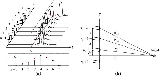
Figure 17.1 Received signals using SAR data collection scheme. (a) Array signal at ![]() . (b) Range between antenna locations and the target.
. (b) Range between antenna locations and the target.
Therefore,
![]() (17.6)
(17.6)
The received signal at ![]() is given by
is given by
 (17.7)
The spatial frequency transform of (17.7) is given by
 (17.8)
where ![]() denotes the spatial frequency, and
denotes the spatial frequency, and ![]() is the target spatial signature at
is the target spatial signature at ![]() such as
such as
 (17.9)
The above analysis shows that separating wall reflections from target reflections amounts to basically separating constant (zero-frequency signal) from nonconstant valued signals across antennas, which can be performed by applying a proper spatial filter.
2.17.2.1.2 Target spatial signature
In the previous section, it is shown that the target signal across the antennas at a fixed time (fixed down-range) is a nonuniformly sampled version of the target reflection. In order to minimize the effect of the wall removal, which is done by spatial filtering, on the target signal, it is necessary to find the target spatial frequency bandwidth as viewed by the array aperture. This is a critical factor in designing the proposed spatial filters for the purpose of wall reflection removal. The target spatial frequency bandwidth depends on the target downrange, as shown in (17.9), and is also inversely proportional to the extent of the target signal return along the array. At any given time, the latter depends on the array length, target down range, and the target signal temporal duration.
Considering a point target, which reflects the radar signal without modification, the target spatial signature can be analytically computed. The minimum bandwidth occurs when the extent of the target return is maximum. Two different cases can be identified depending on the target location in cross-range relative to the edge of the array. Figure 17.2a shows the target signal return in the time-space domain when the target is located within the array aperture, whereas Figure 17.2b shows the case in which the target is outside the array aperture. In these figures, L represents the array length, ![]() is the signal temporal duration, and R is the target range. Consider the case of Figure 17.2a, where
is the signal temporal duration, and R is the target range. Consider the case of Figure 17.2a, where ![]() is the cross-range of the target location from the edge of the array. Without loss of generality, assume that
is the cross-range of the target location from the edge of the array. Without loss of generality, assume that ![]() is larger than or equal to
is larger than or equal to ![]() . The maximum width of the target return across the array for the case of Figure 17.2a is [64]
. The maximum width of the target return across the array for the case of Figure 17.2a is [64]
![]() (17.10)
(17.10)
and for the case of Figure 17.2b,
![]() (17.11)
(17.11)
Figure 17.2 Target return signal in the time-space domain. (a) Target is within the array aperture. (b) Target is outside the array aperture.
In the above equations, ![]() is the radar down-range resolution and
is the radar down-range resolution and
![]() (17.12)
(17.12)
The maximum width is achieved when the target is located along the centerline of the array
![]() (17.13)
(17.13)
Define ![]() as the effective width. Then, the maximum effective width is
as the effective width. Then, the maximum effective width is
![]() (17.14)
(17.14)
and the corresponding minimum frequency bandwidth is given by
![]() (17.15)
(17.15)
Note that ![]() decreases as R increases. This implies that the spatial filter should have a narrower stopband to process the more distant target.
decreases as R increases. This implies that the spatial filter should have a narrower stopband to process the more distant target.
2.17.2.1.3 Moving average wall removal
Moving Average (MA) filter background subtraction is a noncausal Finite impulse response (FIR) filter, which notches out the zero spatial frequency component. The MA subtraction method has been effectively used for removal of the ground reflections in ground penetrating radar [65]. The effect of the MA on the target image can be viewed in the context of the corresponding change in the point spread function (PSF). With the transmitted signal chosen as a stepped-frequency waveform consisting of Q narrowband signals, let ![]() be the signal received at the nth antenna at frequency
be the signal received at the nth antenna at frequency ![]() . Let
. Let ![]() be the signal after MA subtraction. That is
be the signal after MA subtraction. That is
![]() (17.16)
(17.16)
 (17.17)
where 2D + 1 is the filter length. When the sum is taken over the entire length of the array, the moving average becomes just an average over the entire aperture and 2D + 1 = N. The klth pixel value of the image obtained by applying delay-and-sum (DS) beamforming to the received data ![]() is given by
is given by
 (17.18)
where ![]() is the two-way traveling time, through the air and the wall, between the nth antenna and the klth pixel location. The new DS beamforming image after filtering is given by
is the two-way traveling time, through the air and the wall, between the nth antenna and the klth pixel location. The new DS beamforming image after filtering is given by
 (17.19)
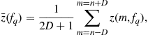
The second term in the above equation is due to the average subtraction. This additional term depends on the signal waveform, target location, and the antenna positions, implying that the effect of average subtraction varies according to these parameters. The PSF is the DS image of a point source as a function of the down-range and the cross-range. Figure 17.3a shows the image of the second term in (17.19) when a point target is located 6 m away from the center of a 3 m long antenna array. In this case, the maximum value is about 0.13 (The maximum value in PSF is one). The signal is a step-frequency waveform covering the 2–3 GHz band with 5 MHz steps. It is noted that the magnitude of this image assumes a high value over a large cross-range area, whereas the down-range spread of the function is small. Figure 17.3b is the PSF without spatial filtering. The modified PSF of the spatial filtered signal, which is the difference between Figure 17.3a and b, is shown in Figure 17.3c. We observe that the size of the mainlobe of the modified PSF remains unchanged with about 0.8 dB loss in the maximum value. However, the sidelobes are higher compared to the original PSF. Although the average subtraction seems to work well in this simulation, the limits of using this subtraction method when handling the distant targets can be shown as follows.
Figure 17.3 Modification in the PSF due to MA subtraction. (a) Second term in (17.19). (b) PSF without filtering. (c) PSF after MA subtraction.
The discrete Fourier transform of ![]() is
is
 (17.20)
Note that
 (17.21)
Therefore,
 (17.22)
As shown above, the subtraction removes the single spatial frequency component ![]() without changing other components. The actual spatial frequency band that is filtered out is always
without changing other components. The actual spatial frequency band that is filtered out is always ![]() , where L is the array length. When
, where L is the array length. When ![]() is equal to L, the target bandwidth is
is equal to L, the target bandwidth is ![]() . In this case, most of the target signal return will be removed by the process of the average subtraction. The range at which
. In this case, most of the target signal return will be removed by the process of the average subtraction. The range at which ![]() is
is
![]() (17.23)
(17.23)
For example, for L = 2 m and ![]() (2 GHz bandwidth),
(2 GHz bandwidth), ![]() is equal to 13.33 m, implying that when the target’s down-range is larger than 13.33 m, the MA subtraction method will eliminate most of the target signature, which is undesirable. Thus, the MA subtraction is simple but produces spatial filter characteristics, which may not be applicable to all wall types and target locations.
is equal to 13.33 m, implying that when the target’s down-range is larger than 13.33 m, the MA subtraction method will eliminate most of the target signature, which is undesirable. Thus, the MA subtraction is simple but produces spatial filter characteristics, which may not be applicable to all wall types and target locations.
2.17.2.1.4 Notch filtering
Zero-phase spatial IIR filters, such as notch filters, are good candidates for wall clutter mitigation. The IIR filter provides a flexible design. It overcomes the problem of the fixed MA (average) filter characteristics that could be unsuitable for various wall and target types and locations. Although the IIR filter spatial extent is truncated because of the finite number of antennas, the filter is still capable of delivering good wall suppression performance without a significant change in the target signal when the number of antennas is moderate. A simple IIR notch filter that rejects zero frequency component is given by
![]() (17.24)
(17.24)
The positive parameter ![]() determines the width of the filter notch. Figure 17.4 shows the frequency response of the filter for various values of
determines the width of the filter notch. Figure 17.4 shows the frequency response of the filter for various values of ![]() and that of MA subtraction with 67 antenna locations. Note the difference between the notch filters and MA. The notch filter does not have ripples and can change its stopband depending on the parameter
and that of MA subtraction with 67 antenna locations. Note the difference between the notch filters and MA. The notch filter does not have ripples and can change its stopband depending on the parameter ![]() . In the underlying problem,
. In the underlying problem, ![]() is the spatial frequency and the parameter
is the spatial frequency and the parameter ![]() provides a compromise between wall suppression and target signal conservation. This flexibility is an advantage of the notch filtering over MA subtraction method. As shown in the figure, as
provides a compromise between wall suppression and target signal conservation. This flexibility is an advantage of the notch filtering over MA subtraction method. As shown in the figure, as ![]() moves closer to one, the stopband becomes narrower such that most of the signal except dc will pass through the filtering.
moves closer to one, the stopband becomes narrower such that most of the signal except dc will pass through the filtering.
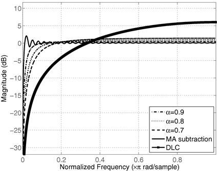
Figure 17.4 Frequency response of the notch filter for various ![]() , DLC with two pulses, and MA subtraction with 67 antennas.
, DLC with two pulses, and MA subtraction with 67 antennas.
The spatial spectrum of wall reflections may have a nonzero width due to unstable antenna path and local inhomogeneities. In this case, a wider filter stopband should be applied to remove most of the wall reflections around dc, but it would also reduce the target reflection. Therefore, the spatial filter should be adjusted to the environment. It is noted that the frequency spectrum of the target reflection depends on the range to the target, the transmitted waveform, and the distance between antenna locations. These parameters determine the sampling point of the received signal and, subsequently, the spatial frequency characteristics of the target. If the sampled target signal does not have a dc component, it will not be severely affected by the spatial filter and, as such, the target image after notch filtering will approximately remain unaltered. It is noted that the desire to have the target spatial spectrum least attenuated by the spatial filtering could play an important role in designing signal waveforms for TWRI.
The filter zero-phase property, which is required for a focused image formation, can be achieved by applying the notch filter twice in the forward and backward directions [66]. By two-way filtering, group delay can be removed. One way to avoid the loss of the target signal returns by filtering, particularly if these returns vary slowly across the array aperture antennas, is to increase the delay between antenna outputs. This is true whether the MA, the notch filter, or any other filter is employed. The increased delay can be achieved by down sampling of sensors without making the sensor spacing too large to cause aliasing. When the antenna positions are down sampled by M, there will be M different sets with ![]() antennas. These M sets are filtered independently and the results are used by the delay and sum beamforming. Figure 17.5 shows the diagram of notch filter processing. The downsampled signal
antennas. These M sets are filtered independently and the results are used by the delay and sum beamforming. Figure 17.5 shows the diagram of notch filter processing. The downsampled signal ![]() for
for ![]() and
and ![]()
![]() (17.25)
(17.25)
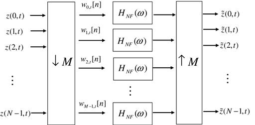
The effective filter length of the IIR filter should be considered when downsampling since the length of the downsampled signal is now ![]() . A highly truncated IIR will lead to undesired filter characteristics.
. A highly truncated IIR will lead to undesired filter characteristics.
2.17.2.1.5 Imaging results
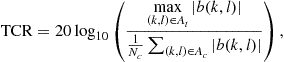
A through-the-wall SAR system was set up in the Radar Imaging Lab at Villanova University. A line array of length 1.2446 m with 0.0187 m inter-element spacing was synthesized, parallel to a 0.14 m thick solid concrete wall, at a standoff distance of 1.01m. The back and the side walls of the room were covered with RF absorbing material to reduce clutter. A stepped-frequency signal covering 1–3 GHz band with 2.75 MHz frequency step was employed. A vertical dihedral was used as the target and was placed 3.04m away on other side of the front wall. The size of each face of the dihedral is 0.39m by 0.28 m. The empty scene without the dihedral target present was also measured for comparison.
First, we examine the validity of the wall EM return assumption that the spatial filtering approach is based on. Figure 17.6a shows the signal reflected from the concrete wall. It clearly shows the first few reflections from the wall and as expected, the wall return assumes almost constant values across the antenna positions. In order to quantify the performance of the images, we apply the target-to-clutter ratio (TCR) which is commonly adopted in SAR image evaluations [67,68]. TCR is similar to the MTI improvement factor, except that the latter is for the time-domain, whereas TCR is for the image domain. TCR is calculated as
 (17.26)
where ![]() is the target area,
is the target area, ![]() is the clutter area, and
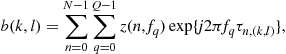
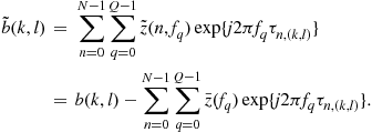
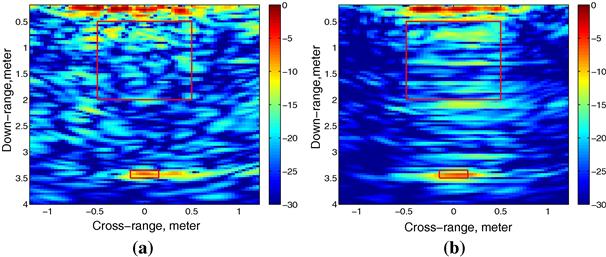
is the clutter area, and ![]() is the number of pixels in the clutter area. TCR, in essence, is the ratio between the maximum pixel value of the target to the average pixel value in the clutter region. The clutter region is the area where no target is present and the wall reflection is severe. The clutter area is manually selected in close vicinity to the wall where wall reflections are most pronounced. The rectangles depicted in the figures represent the clutter area and the target area in our example. Figure 17.6b shows the image without any preprocessing and the target is masked by the wall response. Figure 17.6c shows the result of applying background subtraction, and the target is clearly visible. Figure 17.7a and b demonstrates that the spatial filtering approach is effective in reducing the wall reflections without significantly compromising the target image. Figure 17.7a shows the DS image after MA subtraction, and Figure 17.7b shows the DS image after the notch filtering. TCRs in these figures are 2.2 dB (with wall), 26.2 dB (background subtraction), 13.4 dB (notch filtering), and 15.3 dB (MA subtraction). The background subtracted image provides the highest TCR, while MA subtraction and notch filtering provide comparable performance.
is the number of pixels in the clutter area. TCR, in essence, is the ratio between the maximum pixel value of the target to the average pixel value in the clutter region. The clutter region is the area where no target is present and the wall reflection is severe. The clutter area is manually selected in close vicinity to the wall where wall reflections are most pronounced. The rectangles depicted in the figures represent the clutter area and the target area in our example. Figure 17.6b shows the image without any preprocessing and the target is masked by the wall response. Figure 17.6c shows the result of applying background subtraction, and the target is clearly visible. Figure 17.7a and b demonstrates that the spatial filtering approach is effective in reducing the wall reflections without significantly compromising the target image. Figure 17.7a shows the DS image after MA subtraction, and Figure 17.7b shows the DS image after the notch filtering. TCRs in these figures are 2.2 dB (with wall), 26.2 dB (background subtraction), 13.4 dB (notch filtering), and 15.3 dB (MA subtraction). The background subtracted image provides the highest TCR, while MA subtraction and notch filtering provide comparable performance.
2.17.2.2 Wall parameter estimation, modeling, and subtraction
2.17.2.2.1 Approach
In this approach, the effect of the wall on EM wave propagation is achieved through three steps. The wall parameters are accurately estimated. Then, the reflected signal from the wall is properly modeled. Finally, the modeled signal is subtracted from the measured signal.
Building walls, such as brick, adobe, and poured concrete walls, can be modeled by homogeneous dielectric slabs. Using the geometric optics approach, the reflection coefficient ![]() for vertically and horizontally polarized incident waves through the wall is given by [44,69]
for vertically and horizontally polarized incident waves through the wall is given by [44,69]
 (17.27)
where ![]() for horizontal polarization and
for horizontal polarization and ![]() for vertical polarization of the incident fields. In (17.27),
for vertical polarization of the incident fields. In (17.27), ![]() is the relative dielectric constant, d is the thickness of the wall, and
is the relative dielectric constant, d is the thickness of the wall, and ![]() and
and ![]() are the normal components of the propagation constants in air and in the dielectric, respectively. The expressions for the vertical/transverse magnetic and horizontal/transverse electric unit vectors are given in [69].
are the normal components of the propagation constants in air and in the dielectric, respectively. The expressions for the vertical/transverse magnetic and horizontal/transverse electric unit vectors are given in [69].
The wall parameters can be estimated from the time-domain backscatter at a given location [44,70]. Basically, the response of the wall is gated from the total backscatter signal and transferred to the frequency domain. The mean-squared error between the calculated reflection coefficient ![]() of (17.27) and the measured reflection coefficient
of (17.27) and the measured reflection coefficient ![]() given by
given by
 (17.28)
is computed, and its minimum is searched for the wall thickness and permittivity [44,71]. In (17.28), ![]() is the number of frequency points and
is the number of frequency points and ![]() is the nth frequency.
is the nth frequency.
The estimated wall parameters are then used to compute the wall EM reflection. This could be accomplished either numerically using EM modeling software, or in case of far-field conditions, analytically using the following expression [44]
![]() (17.29)
(17.29)
where ![]() is the standoff distance of the radar from the wall,
is the standoff distance of the radar from the wall, ![]() is the wavelength, G is the antenna gain,
is the wavelength, G is the antenna gain, ![]() is the nth wave constant, c is the speed of light in free space, and
is the nth wave constant, c is the speed of light in free space, and ![]() is the reflectivity matrix from the wall at normal incidence angle and is given by,
is the reflectivity matrix from the wall at normal incidence angle and is given by,
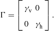 (17.30)
In (17.30), the subscripts “v” and “h,” respectively, denote the vertical and horizontal polarization and ![]() is given by (17.27). This estimated wall reflection should be coherently subtracted from the total received signal in order to isolate the signature of the target on the other side of the wall.
is given by (17.27). This estimated wall reflection should be coherently subtracted from the total received signal in order to isolate the signature of the target on the other side of the wall.
The isolated target return can then be processed to generate an image of the scene. The effects of the wall transmissivity on the target image are the following: (1) dislocation of the target from its actual position in range and (2) significant degradation in cross-range resolution [41,44]. To compensate for the effects of transmission through the wall, a compensation factor proportional to the inverse of the squared of the wall transmittivity can be used in the conventional free-space image formation methods. In cases where transmissivity is low and the signal is noisy, division by a small noise-affected number may cause significant distortion. In such cases, one may use only the phase of transmission coefficients as a compensation factor [44].
2.17.2.2.2 Imaging results
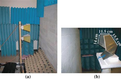
An experimental study was conducted at the Radiation Laboratory in University of Michigan. The measurement setup consists of an HP8753D vector network analyzer, two double ridge horn antennas with operational frequency range of 1–18 GHz, an XY table along with a control unit, and a personal computer. The vertically aligned antennas, one for transmission and the other for reception, are mounted on a vertical wooden rod (along the z-axis), which is attached to the carriage of the XY table. A 2.37 m ![]() 1.77 m wall composed of poured concrete blocks is made on top of a layer of cinder blocks inside the laboratory. The underlying cinder block layer is used to line up the antennas in height at approximately the middle of the concrete block wall. Figure 17.8a shows the side view of the measurement setup. A small trihedral corner reflector with pentagonal panel geometry is used as a point target behind the wall, as shown in Figure 17.8b. The back corner of the trihedral (scattering phase center) is at x = −0.71 m and at the same height as that of the receiver antenna, i.e., 1.28 m above the ground plane. The transmitting antenna is attached about 0.25 m below the receiving antenna on the wooden rod. The antennas are moved along a scan line of length 95.88 cm, parallel to the wall, with a spacing of 2.04 cm. The apertures of both antennas are about 0.45 m away from the wall. The frequency of operation is from 1 to 2.5 GHz and the frequency step is 12.5 MHz. It is noted that the antennas are in the far-field region of the target.
1.77 m wall composed of poured concrete blocks is made on top of a layer of cinder blocks inside the laboratory. The underlying cinder block layer is used to line up the antennas in height at approximately the middle of the concrete block wall. Figure 17.8a shows the side view of the measurement setup. A small trihedral corner reflector with pentagonal panel geometry is used as a point target behind the wall, as shown in Figure 17.8b. The back corner of the trihedral (scattering phase center) is at x = −0.71 m and at the same height as that of the receiver antenna, i.e., 1.28 m above the ground plane. The transmitting antenna is attached about 0.25 m below the receiving antenna on the wooden rod. The antennas are moved along a scan line of length 95.88 cm, parallel to the wall, with a spacing of 2.04 cm. The apertures of both antennas are about 0.45 m away from the wall. The frequency of operation is from 1 to 2.5 GHz and the frequency step is 12.5 MHz. It is noted that the antennas are in the far-field region of the target.
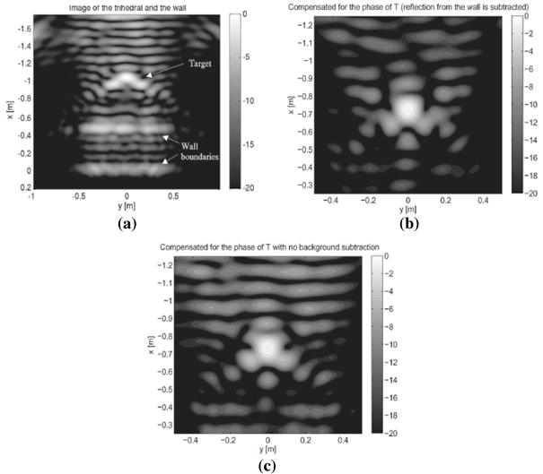
An image is first constructed under assumption of free-space propagation by using the total received signal, and is shown in Figure 17.9a. Here, in addition to the target, the wall is also imaged, primarily as two parallel lines showing the front and back boundaries. Since backscatter from the wall is very strong, the sidelobes generated by image formation spill over into desired image domain, which is manifested as multiple lines parallel to the wall surfaces. Also, the target appears blurred and its location is biased. Figure 17.9b shows the image after the estimate, model, and subtract approach was applied. The wall thickness and the permittivity were estimated using (17.28) as 20 cm and 5.7 + j0.6, respectively. The wall reflection was computed using (17.29) and subtracted from the total received signal, and the resulting signal was used for image formation. For comparison, the signal prior to wall return subtraction was used for imaging wherein compensation for the effect of transmission through the wall was applied and is shown in Figure 17.9c. Although the imaged target is at the correct location and is refocused in Figure 17.9c, existence of the wall sidelobes in the image is still evident. By comparing Figure 17.9b and c, a substantial improvement in clutter rejection is observed after subtraction of the modeled wall return.
2.17.3 Multipath exploitation
The existence of targets inside a room or in an enclosed structure introduces multipath in the radar return, which results in false targets or ghosts in the radar images. These ghosts lie on or near the vicinity of the back and side walls, leading to a cluttered image with several false positives. Without a reasonable through-the-wall multipath model, it becomes difficult to associate a ghost to a particular target. Identifying the nature of the targets in the image and tagging the ghosts with their respective target according to a developed multipath model, although important to reduce false alarms, is not the final goal of a high-performance through-the-wall imaging system. Since each multipath provides some information about the target, it becomes prudent to utilize the multipath rather than ignoring it, once identified. The utilization or exploitation of the multipath to one’s advantage represents a paradigm shift when compared to the classical approach of either ignoring or mitigating it.
For through-the-wall radar imaging applications, the existence of multipath has been recently demonstrated for stationary targets in [52,72,73]. In [72], the authors use distributed fusion to remove the false targets caused either from multipath or target interactions for stationary scenes after suitable image registration. In [52], time reversal techniques are used to alleviate ghosts and clutter from the target scene and in [73], a synthetic aperture radar (SAR) based image of a human inside a room is shown along with possible multipath ghosts. However, no more rigorous multipath modeling and analysis are presented in the aforementioned references [52,72,73] and the references therein.
In this section, we derive a model for the multipath in an enclosed room of four walls. The model considers propagation through a front wall and specular reflections at interior walls. A SAR system is considered and stationary or slow moving targets are assumed. Although the multipath model presented deals with walls, reflections from the ceiling and floor can be readily handled. We demonstrate analytically that the multipath as seen by each sensor is displaced, and, therefore, we derive the actual focusing positions of the multipath ghosts in downrange and crossrange. The multipath model permits an implementation of a multipath exploitation algorithm, which associates as well as maps each target ghost back to its corresponding true target location. In so doing, the exploitation algorithm improves the radar system performance by ameliorating the false positives in the original SAR image as well as increasing the signal-to-clutter ratio (SCR) at the target locations, culminating in enhanced behind the wall target detection and localization. It is noted that the exploitation algorithm only maps back target-wall interactions; target-target interactions are left untreated. The multipath exploitation algorithm is inspired by the work in [74], wherein the shadowed regions of a target are revealed via its multipath returns. The difference, however, is that we are not striving to reveal the shadowed regions of the target. In our case, we deal with targets with arbitrary dielectric constants, and wish to associate and map each multipath to its true target location.
2.17.3.1 Image formation algorithm
In this section, we describe the through-the-wall delay-and-sum beamforming approach [40,41,75,76]. We consider a SAR system in which a single antenna at one location transmits a wideband signal and receives the radar return, and then moves to the next location and repeats the same operation along the axis parallel to the front wall. Assume N monostatic antenna locations. The setup is as depicted in Figure 17.10. Consider a single point target, located at ![]() . At each antenna location, the radar transmits a pulsed waveform
. At each antenna location, the radar transmits a pulsed waveform ![]() , where “t” indexes the time within the pulse, and measures the reflected signal. The target return at the
, where “t” indexes the time within the pulse, and measures the reflected signal. The target return at the ![]() th antenna location is given by,
th antenna location is given by,
![]() (17.31)
(17.31)
where ![]() represents the target reflectivity,
represents the target reflectivity, ![]() is the complex amplitude associated with the one-way propagation through a dielectric wall for the
is the complex amplitude associated with the one-way propagation through a dielectric wall for the ![]() th antenna location [77], and
th antenna location [77], and ![]() represents the one-way through-the-wall propagation delay from the
represents the one-way through-the-wall propagation delay from the ![]() th antenna location to the target.
th antenna location to the target.
The scene of interest comprises several pixels indexed by the downrange and the crossrange. The complex composite return from the ![]() th pixel location
th pixel location ![]() is obtained by applying time delays to the N received signals, followed by weighting and summing the results. That is,
is obtained by applying time delays to the N received signals, followed by weighting and summing the results. That is,
 (17.32)
The signal ![]() is passed through a matched filter, with impulse response
is passed through a matched filter, with impulse response ![]() . The complex amplitude assumed by the pixel
. The complex amplitude assumed by the pixel ![]() in the image
in the image ![]() is obtained by sampling the matched filter output at time
is obtained by sampling the matched filter output at time ![]() ,
,
![]() (17.33)
(17.33)
where “![]() ” denotes the convolution operation. Equations (17.32) and (17.33) describe the standard beamforming approach in through-the-wall radar imaging. It is noted that if the imaged pixel is in the vicinity of or at the true target location, then the complex amplitude in (17.33) assumes a high value as given by the system’s point spread function. The process described in (17.32) and (17.33) is carried out for all pixels in the scene of interest to generate the image of the scene.
” denotes the convolution operation. Equations (17.32) and (17.33) describe the standard beamforming approach in through-the-wall radar imaging. It is noted that if the imaged pixel is in the vicinity of or at the true target location, then the complex amplitude in (17.33) assumes a high value as given by the system’s point spread function. The process described in (17.32) and (17.33) is carried out for all pixels in the scene of interest to generate the image of the scene.
The beamforming approach as described above is pertinent to a point target in a two-dimensional (2D) scene. Extensions to three-dimensional (3D) scenes and spatially extended targets are discussed in [40,78]. It is noted that, in the above beamforming description, we have not considered the multipath returns; neither have we addressed the specificities of calculating the delays, ![]() , which will be treated in detail in the following sections. Without loss of generality, we now assume that the weights
, which will be treated in detail in the following sections. Without loss of generality, we now assume that the weights ![]() and the target has unit reflectivity.
and the target has unit reflectivity.
2.17.3.2 Multipath model
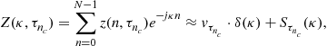
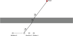
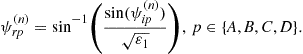
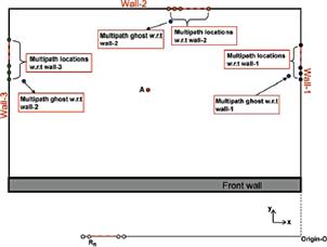
Consider a room under surveillance using a SAR system. A priori knowledge of the room layout, i.e., wall locations and material properties, is assumed. The scene being observed relative to the ![]() th sensor location is as shown in Figure 17.11. The origin is marked as point “O” in the figure, and the standard convention for the positive x- and y- axes is assumed. The
th sensor location is as shown in Figure 17.11. The origin is marked as point “O” in the figure, and the standard convention for the positive x- and y- axes is assumed. The ![]() th sensor location is given by
th sensor location is given by ![]() The front wall has a thickness
The front wall has a thickness ![]() and dielectric constant
and dielectric constant ![]() . For notational simplicity, the back and the side walls are also assumed to have
. For notational simplicity, the back and the side walls are also assumed to have ![]() as the dielectric constant. The side walls, labeled as wall-1 and wall-3, have a length
as the dielectric constant. The side walls, labeled as wall-1 and wall-3, have a length ![]() , whereas the front wall and the back wall (wall-2) have a length
, whereas the front wall and the back wall (wall-2) have a length ![]() . The target is stationary and at location
. The target is stationary and at location ![]() . The standoff distance from the front wall is constant for each sensor location constituting the synthetic aperture, and is denoted as
. The standoff distance from the front wall is constant for each sensor location constituting the synthetic aperture, and is denoted as ![]() . In the figure, we consider the direct path, referred to as path-A, and three additional paths, namely, paths-B, C, and D, which correspond to single-bounce multipath. In general, there exist other paths which can contribute to the multipath returns; these include multiple bounces from the back and side walls as well as paths that include multiple reflections within each of the four walls themselves. Examples of the former and the latter are provided in Figure 17.12. Such paths are defined as higher-order multipath. Hence, in Figure 17.11, we have considered only first-order multipath. It is noted that higher-order multipath are in general weaker compared to the first-order multipath due to the secondary reflections and refractions at the various air-wall interfaces and high attenuation in the wall material. Therefore, we choose to exclude these paths from the model.
. In the figure, we consider the direct path, referred to as path-A, and three additional paths, namely, paths-B, C, and D, which correspond to single-bounce multipath. In general, there exist other paths which can contribute to the multipath returns; these include multiple bounces from the back and side walls as well as paths that include multiple reflections within each of the four walls themselves. Examples of the former and the latter are provided in Figure 17.12. Such paths are defined as higher-order multipath. Hence, in Figure 17.11, we have considered only first-order multipath. It is noted that higher-order multipath are in general weaker compared to the first-order multipath due to the secondary reflections and refractions at the various air-wall interfaces and high attenuation in the wall material. Therefore, we choose to exclude these paths from the model.

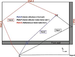
The walls are assumed smooth with specular reflections. The smoothness assumption is valid, since for through-the-wall radars, the wavelength of operation is much larger than the roughness of the walls. Specular reflections are a direct consequence of the wall smoothness, and necessitate that the angle of incidence be equal to the angle of reflection. Note that, in general, the back and side walls may each be of a different material (interior or exterior grade), and thus may assume different values for the wall thickness and dielectric constant. If interior reflections inside these walls are considered, then the thickness of these walls is required [52,73,74]. However, since we have ignored such higher-order paths, we only require the dielectric constant of the back and side walls to be known. As the EM wave propagates through the front wall, it bends at the medium discontinuity as dictated by Snell’s law, i.e., each of the paths, as seen in Figure 17.11, has an associated angle of incidence and an angle of refraction. For example, the angles of incidence and refraction for path-B are denoted as ![]() and
and ![]() , respectively. Similar nomenclature follows for the remaining paths.
, respectively. Similar nomenclature follows for the remaining paths.
Let the reflection points on wall-1, 2, and 3 be denoted by ![]() , and
, and ![]() , with respective position vectors
, with respective position vectors ![]() , and
, and ![]() . It is clear that these position vectors are dependent on the sensor location. The one-way path delays for the four paths, with the antenna at the
. It is clear that these position vectors are dependent on the sensor location. The one-way path delays for the four paths, with the antenna at the ![]() th location, are denoted by
th location, are denoted by ![]() , and can be derived from the geometry as
, and can be derived from the geometry as
 (17.34)
with c being the speed of light and the coordinates of ![]() , and
, and ![]() given by
given by
 (17.35)
Equations (17.34) and (17.35) depend on the angles of incidence and refraction. Since the standoff distance is a known constant, by projecting the various paths to the x-axis, we obtain the following equations, which are useful in calculating the various angles.
 (17.36)
![]()
The angles of refraction can be determined from Snell’s law as,
 (17.37)
Substituting the angles of refraction from (17.37) in (17.36), and using (17.35), we obtain a set of equations that can be solved numerically for the angles of incidence by using the Newton method. The angles of refraction can then be obtained using (17.37).
We are now in a position to write the radar signal return from the single target scene as a superposition of the direct path and the multipath returns. For the ![]() th sensor location, we obtain
th sensor location, we obtain
 (17.38)
where ![]() is the complex amplitude associated with reflection and transmission coefficients for the one-way propagation along path-p, and depends on the angles of incidence, the angles of refraction, and dielectric properties of the walls [77]. In (17.38), the first summation captures the two-way returns along the direct path and each multipath. More specifically, the signal propagates along a particular path-p,
is the complex amplitude associated with reflection and transmission coefficients for the one-way propagation along path-p, and depends on the angles of incidence, the angles of refraction, and dielectric properties of the walls [77]. In (17.38), the first summation captures the two-way returns along the direct path and each multipath. More specifically, the signal propagates along a particular path-p, ![]() , reaches the target and retraces the same path back to the radar, i.e., path-p. The multipath returns due to the combination paths are captured by the second summation, i.e., the wave initially travels to the target via path-p and returns to the radar through a different path-q,
, reaches the target and retraces the same path back to the radar, i.e., path-p. The multipath returns due to the combination paths are captured by the second summation, i.e., the wave initially travels to the target via path-p and returns to the radar through a different path-q, ![]()
From Figure 17.11 and (17.35), we observe that the coordinates of the points of reflection at the back and side walls are sensor dependent, implying that the multipath presents itself at different locations to the different sensors. Location of the multipath as seen by each sensor and the actual focusing position of the resulting ghost in the image are discussed next.
2.17.3.2.1 Multipath locations
For simplicity of analysis, consider the scenario in Figure 17.11, but without the front wall. We first focus on the multipath originating from wall-1, i.e., the signal traveling to the target via path-A, and following path-B back to the radar or vice versa. The goal is to find the location of the multipath corresponding to the above combination path as seen by each of theN sensors. Let the point ![]() , represented by the vector
, represented by the vector ![]() , denote the multipath location as seen by the
, denote the multipath location as seen by the ![]() th sensor. The superscript “
th sensor. The superscript “![]() ” stresses that the multipath is associated with the reflection at wall-1 and the subscript “t” indicates that the multipath is due to the target located at
” stresses that the multipath is associated with the reflection at wall-1 and the subscript “t” indicates that the multipath is due to the target located at ![]() . Reflecting path-B about wall-1 yields an alternate radar-target geometry, as shown in Figure 17.13. We obtain the virtual target denoted by point
. Reflecting path-B about wall-1 yields an alternate radar-target geometry, as shown in Figure 17.13. We obtain the virtual target denoted by point ![]() with coordinates
with coordinates ![]() such that the distance
such that the distance ![]() , which implies that
, which implies that
![]() (17.39)
(17.39)

In other words, the combination path comprising of path-A and path-B has the same length as path-A and the path connecting the ![]() th sensor to the virtual target at
th sensor to the virtual target at ![]() . Due to the monostatic nature of the radar system, this combination path appears to the
. Due to the monostatic nature of the radar system, this combination path appears to the ![]() th sensor as the traditional two way path of length
th sensor as the traditional two way path of length ![]() . Therefore, we have
. Therefore, we have
![]() (17.40)
(17.40)
Additionally, we obtain the virtual radar at ![]() on the other side of the wall, as shown in Figure 17.13. Considering Figure 17.13, it is readily observed that the first order multipath has the same time delay as a bistatic configuration, comprising the radar and the virtual radar. That is, in terms of range, we have
on the other side of the wall, as shown in Figure 17.13. Considering Figure 17.13, it is readily observed that the first order multipath has the same time delay as a bistatic configuration, comprising the radar and the virtual radar. That is, in terms of range, we have
![]() (17.41)
(17.41)
where ![]() represents the bistatic configuration. In the bistatic case, the constant range contour corresponding to the multipath is an ellipse, which has foci at the radar and virtual radar and passes through the target and the virtual target locations. On the other hand, the monostatic measurement scenario described by (17.40) has a circular constant range contour, centered at the radar. Since the two measurements are equivalent, the location of the multipath corresponds to the point of intersection of the bistatic elliptical and the monostatic circular constant range contours. The equations for the ellipse and circle are given by
represents the bistatic configuration. In the bistatic case, the constant range contour corresponding to the multipath is an ellipse, which has foci at the radar and virtual radar and passes through the target and the virtual target locations. On the other hand, the monostatic measurement scenario described by (17.40) has a circular constant range contour, centered at the radar. Since the two measurements are equivalent, the location of the multipath corresponds to the point of intersection of the bistatic elliptical and the monostatic circular constant range contours. The equations for the ellipse and circle are given by
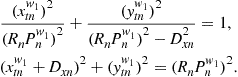 (17.42)
Solving (17.42) for an intersection point, we can readily see that ![]() is the only solution. In other words, regardless of the location of the target, its first-order multipath always falls on the wall. The y-coordinate of
is the only solution. In other words, regardless of the location of the target, its first-order multipath always falls on the wall. The y-coordinate of ![]() can then be derived as
can then be derived as
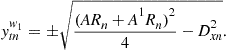 (17.43)
In (17.43), the positive y-coordinate is the desired value as the other solution lies behind the radar. It is clear from (17.43) that the multipath location is sensor dependent. Therefore, the locations of the target multipath corresponding to the various sensor positions will be displaced from one another. In the presence of the front wall, the multipath remains on the wall, but the equations for the ellipse and circle are different than that presented in (17.42). Hence, for the scenario comprising of the front-wall and wall-1, the multipath appears on wall-1, with its y-coordinate given by
 (17.44)
where ![]() and
and ![]() are, respectively, the angles of incidence and refraction for the ghost. The solution in (17.44) depends on the angle
are, respectively, the angles of incidence and refraction for the ghost. The solution in (17.44) depends on the angle ![]() , which can be obtained by solving
, which can be obtained by solving
 (17.45)
So far, we have considered the multipath corresponding to wall-1; there exist two other multipath returns tagged to the remaining walls, namely, wall-2, and wall-3. We can readily show, using similar analysis, that the multipath associated with wall-2 appears on wall-2, i.e., ![]() , at an x-coordinate given by
, at an x-coordinate given by
 (17.46)
The angles in the above equation are determined by solving the equations,
 (17.47)
Likewise, the multipath associated with wall-3 appears at wall-3, i.e., ![]() , and at a y-coordinate given by,
, and at a y-coordinate given by,
 (17.48)
The respective angles can be obtained by solving,
 (17.49)
From the above equations, it is again observed that the N sensors view the multipath, resulting from the combination paths associated with a particular wall, at different locations on that wall. That is, the multipath maybe regarded as a moving target. As a result, when applying beamforming, the multipath ghost appears at a different pixel in the vicinity of the true multipath locations. We note that the multipath ghost will lie inside the room except when the target is near the corners of the room. In this case, as the multipath corresponding to the N sensors may appear along an extrapolation of the wall, the multipath ghost may appear outside the room. We further note that the virtual target corresponds to two-way propagation along the single-bounce multipath, and is readily seen to lie outside the room perimeter. The multipath focusing pixel analysis for the combination paths is discussed next.
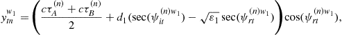
2.17.3.2.2 Multipath focusing analysis
Consider Figure 17.14, which shows the multipath locations w.r.t to walls-1–3, and the focusing pixels w.r.t to these walls. Consider the multipath locations associated with wall-1; further assume that the focused multipath ghost appears at a pixel location given by
![]() (17.50)
(17.50)
where ![]() is the true multipath location corresponding to the first sensor position. Using a first order Taylor series expansion, which is valid under conditions of a small aperture [79] and when the ghost is in the vicinity of the true multipath locations, we obtain the difference in propagation path length between the multipath ghost location and the true multipath location w.r.t the first sensor position as
is the true multipath location corresponding to the first sensor position. Using a first order Taylor series expansion, which is valid under conditions of a small aperture [79] and when the ghost is in the vicinity of the true multipath locations, we obtain the difference in propagation path length between the multipath ghost location and the true multipath location w.r.t the first sensor position as
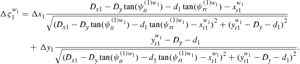 (17.51)
Following the analysis in [79], (17.51) can be expressed as
![]() (17.52)
(17.52)
In general, for the ![]() th sensor, we have
th sensor, we have
![]() (17.53)
(17.53)
For the multipath to focus at the location ![]() , we must have,
, we must have,
![]() (17.54)
(17.54)
This yields a least squares (LS) formulation, given by
 (17.55)
where “![]() ” denotes the Hadamard or element-wise product. The solution of (17.55) is readily obtained by
” denotes the Hadamard or element-wise product. The solution of (17.55) is readily obtained by ![]() .
.
Now, considering the multipath w.r.t wall-2, we have the following LS formulation for the focused ghost pixel.
 (17.56)
![]()
Similarly, for the multipath from wall-3, we have
 (17.57)
The formulations in (17.56)–(17.58) assume that the sensor position increases from left to right. In other words, sensor-1 is at the far left of the array whereas sensor-N is at the far right.
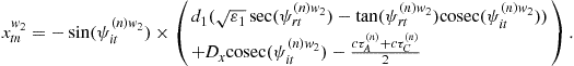
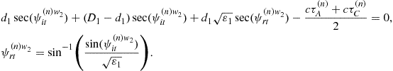
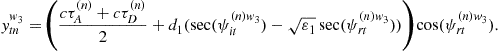
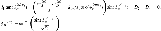
2.17.3.3 Multipath exploitation algorithm
Noting that the multipath ghosts exist due to the presence of the target, we state our objective as follows. Given the beamformed image ![]() , our aim is to associate each multipath ghost with the respective target via the model developed in Section 2.17.3.2. The principle is captured in Figure 17.15, which consists of two targets and six false positives or multipath ghosts. We desire to associate and map these ghosts to their respective true target locations. The main advantages of such an association or mapping are reduction in false positives in the original beamformed image, and an increase in the SCR at the true target coordinates. Note that the first advantage is directly implied in Figure 17.15, whereas the second advantage is explained as follows.
, our aim is to associate each multipath ghost with the respective target via the model developed in Section 2.17.3.2. The principle is captured in Figure 17.15, which consists of two targets and six false positives or multipath ghosts. We desire to associate and map these ghosts to their respective true target locations. The main advantages of such an association or mapping are reduction in false positives in the original beamformed image, and an increase in the SCR at the true target coordinates. Note that the first advantage is directly implied in Figure 17.15, whereas the second advantage is explained as follows.

For ease of exposition, the technique is explained considering the focused multipath ghost from wall-1 only. The technique for exploiting all the ghosts w.r.t to all three walls is enumerated subsequently. Consider an arbitrary pixel location ![]() , whose focused multipath ghost w.r.t wall-1 presents itself at location
, whose focused multipath ghost w.r.t wall-1 presents itself at location ![]() . Consider an intermediate image,
. Consider an intermediate image, ![]() , wherein the association and mapping of the focused multipath ghosts is performed using simple 2D weighting functions. That is,
, wherein the association and mapping of the focused multipath ghosts is performed using simple 2D weighting functions. That is,
 (17.58)
where ![]() and
and ![]() are the weighting functions and
are the weighting functions and ![]() is an arbitrary variance. The weighting functions are related to the two dimensional real Gaussian distributions. A natural improvement, albeit not pursued here, is to let the variance in the y-direction to be equal to the system’s range resolution, the variance in the x-direction to be equal to the system’s crossrange resolution, and introducing a correlation which is a function of the actual ghost location. This would ensure that the ensuing weighting functions are rotated and sheared to match the system’s point spread function, nevertheless at a higher computational cost. The role of
is an arbitrary variance. The weighting functions are related to the two dimensional real Gaussian distributions. A natural improvement, albeit not pursued here, is to let the variance in the y-direction to be equal to the system’s range resolution, the variance in the x-direction to be equal to the system’s crossrange resolution, and introducing a correlation which is a function of the actual ghost location. This would ensure that the ensuing weighting functions are rotated and sheared to match the system’s point spread function, nevertheless at a higher computational cost. The role of ![]() and
and ![]() is explained as follows. Consider the weighting function
is explained as follows. Consider the weighting function ![]() ; if the pixel
; if the pixel ![]() is in the vicinity of the focused multipath ghost pixel
is in the vicinity of the focused multipath ghost pixel ![]() associated with the target location
associated with the target location ![]() , then
, then ![]() assumes a large value. On the other hand, if
assumes a large value. On the other hand, if ![]() is not in the vicinity of
is not in the vicinity of ![]() , then
, then ![]() assumes a low value. Since an exponential function is used, the weights are always between 0 and 1, the lower bound being theoretically unachievable. The vicinity is obviously controlled by the variance parameter,
assumes a low value. Since an exponential function is used, the weights are always between 0 and 1, the lower bound being theoretically unachievable. The vicinity is obviously controlled by the variance parameter, ![]() . From our extensive simulations, we found that a lower variance must be chosen for smaller dimension rooms. For small rooms, it is logical to assume that the ghosts and higher order multipath are located quite close to one another. Therefore, it becomes prudent to be conservative in selecting the variances. Large variances for smaller rooms lead to false mappings. Thus, variance selection for the problem at hand must be guided by the actual dimensions of the room being imaged. The weighting function
. From our extensive simulations, we found that a lower variance must be chosen for smaller dimension rooms. For small rooms, it is logical to assume that the ghosts and higher order multipath are located quite close to one another. Therefore, it becomes prudent to be conservative in selecting the variances. Large variances for smaller rooms lead to false mappings. Thus, variance selection for the problem at hand must be guided by the actual dimensions of the room being imaged. The weighting function ![]() rejects pixel locations at and in the vicinity of the imaged pixel, i.e., the location corresponding to the assumed true target location
rejects pixel locations at and in the vicinity of the imaged pixel, i.e., the location corresponding to the assumed true target location ![]() . This is required because, although the focus point is singular, but due to the system’s point spread function, some of the energy is spread to the neighboring pixels.
. This is required because, although the focus point is singular, but due to the system’s point spread function, some of the energy is spread to the neighboring pixels.
From our extensive simulations, we found that as the original image ![]() is complex-valued, summing or integrating across the multipath pixels may result in destructive interference yielding a poor SCR. This loss of SCR is against our principle of multipath exploitation. To alleviate this problem, we use the intensity of the original beamformed image in (17.58) as
is complex-valued, summing or integrating across the multipath pixels may result in destructive interference yielding a poor SCR. This loss of SCR is against our principle of multipath exploitation. To alleviate this problem, we use the intensity of the original beamformed image in (17.58) as
 (17.59)
which implies an incoherent summation. Now considering the ghosts w.r.t the three walls, we can readily see that (17.59) is modified as
 (17.60)
Image ![]() will have no intensity at and near the vicinity of the focused multipath pixels. Hence, consider the following composite image obtained by simple pixel-wise multiplication.
will have no intensity at and near the vicinity of the focused multipath pixels. Hence, consider the following composite image obtained by simple pixel-wise multiplication.
![]() (17.61)
(17.61)
The effect of pixel-wise multiplication in (17.61) is as follows. The image ![]() will have deep nulls at the hypothesized ghosts locations, whereas a large peak at the true target location. Thus, (17.61) is essentially a masking operation, nulling the ghosts in the original image
will have deep nulls at the hypothesized ghosts locations, whereas a large peak at the true target location. Thus, (17.61) is essentially a masking operation, nulling the ghosts in the original image ![]() , and simultaneously enhancing the energy at the true target location. Hence, the composite image
, and simultaneously enhancing the energy at the true target location. Hence, the composite image ![]() will alleviate the false positives, i.e., the multipath ghosts and increase the intensity of the true target pixel. In the approach described, the multipath ghost locations are readily obtained using the multipath focusing analysis in Section 2.17.3.2.2.
will alleviate the false positives, i.e., the multipath ghosts and increase the intensity of the true target pixel. In the approach described, the multipath ghost locations are readily obtained using the multipath focusing analysis in Section 2.17.3.2.2.
It is noted that, in practice, different targets may exhibit significantly weaker bistatic radar cross sections (RCS) relative to their monostatic RCS. Accordingly, some or maybe all of the target ghosts may go unnoticed. In this case, the proposed multipath exploitation approach will not prove beneficial as there may not be any increase in the target SCR. Also, consider a scenario where one target presents itself at one of the other target’s focused multipath ghost. Since multipath is unexploited in the original beamformed image, we would declare the presence of the target at the pixel in question. On the other hand, the proposed approach will map this target and of course the collocated multipath ghost back to the other target’s location causing the second target to go undetected. The question then arises whether one should ignore the multipath ghosts and consider them as true targets or instead exploit the multipath ghosts. The former has an unreasonably high false alarm rate, whereas the latter yields poor target detection for the considered scenario, which, although rare, can occur in practice. However, noting that indoor targets of interest are typically in motion, it is reasonable to assume that a genuine target would not persist on a multipath ghost throughout the surveillance period. Hence, multipath exploitation should be preferred. Another scenario of interest is when the direct path to the target is blocked. In that case, although the ghosts will be mapped to the true target coordinates in the image ![]() , the masking operation in (17.61) will cause the target to still go undetected as the original image
, the masking operation in (17.61) will cause the target to still go undetected as the original image ![]() will have a null at the target location.
will have a null at the target location.
2.17.3.4 Experimental results
A through-the-wall SAR system was set up in the Radar Imaging Lab at Villanova University. A stepped-frequency signal with 696 steps covering the 1–3 GHz frequency band was used. This provides a range resolution of 0.15 m and a maximum unambiguous range of 40 m. The room dimensions are ![]() and
and ![]() . The side walls and part of the floor were covered with RF absorbers and only multipath due to the back wall was considered. The front wall is made of 0.15m thick solid concrete blocks with a dielectric constant of 7.66. The synthetic aperture consisted of an 81-element monostatic linear array with an inter-element spacing of 2.22cm. The standoff distance of the array from the front wall is 1.53m. The experimental set up is depicted in Figure 17.16.
. The side walls and part of the floor were covered with RF absorbers and only multipath due to the back wall was considered. The front wall is made of 0.15m thick solid concrete blocks with a dielectric constant of 7.66. The synthetic aperture consisted of an 81-element monostatic linear array with an inter-element spacing of 2.22cm. The standoff distance of the array from the front wall is 1.53m. The experimental set up is depicted in Figure 17.16.

Two different experiments were conducted. In the first experiment, a 0.35m diameter metal sphere, labeled as “Target 1” in Figure 17.16, was used as a target. The second experiment consisted of two targets, the first being the sphere used in the single target case, while the second, labeled as “Target 2” in Figure 17.16, was a smaller metallic sphere of 0.2032 m diameter. An empty scene measurement without the targets present in the scene was also made and was coherently subtracted from the target scene data to reduce the clutter. The beamformed image corresponding to the single target scene is depicted in Figure 17.17a; both the target and the ghost are clearly visible in the image. In addition, other target-room interactions, such as those resulting from multiple bounces within the front wall, can be observed. The result after multipath exploitation is provided in Figure 17.17b. The variance of the weighting functions in the exploitation algorithm was chosen to be equal to the system’s range resolution. We observe that as expected, the ghost has been correctly mapped back to the target, while the other target-room interactions are left as is in the exploited image. Figure 17.18a shows the beamformed image corresponding to the two target scene. Both targets as well as the two ghosts with respect to the back wall are clearly seen. The multipath exploited image is provided in Figure 17.18b, in which one can see that the ghosts have been mapped back to the target locations. We note that, similar to the single target case, the other target-room and target-target interactions are retained in Figure 17.18b.

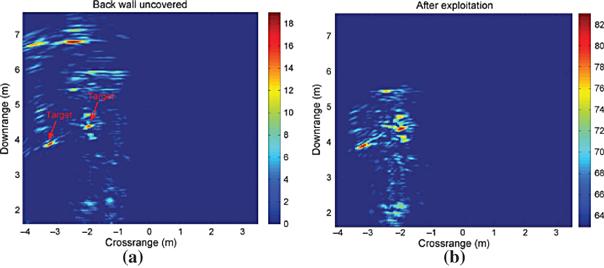
2.17.4 Change detection based MTI approach
Detection of humans is one of the most important objectives in urban sensing and through-the-wall radar technology [13,14,27,73,80–82]. Humans belong to the class of animate objects which are characterized by motion of the limbs, breathing, and heartbeat. These features separate animate and inanimate objects and allow the detection of targets of interest to proceed based on changes in the phase of the scattered radar signals over successive probing and data observations.
Change detection techniques have been recently used to detect moving targets in the presence of heavy clutter that is caused by strong reflections from exterior and interior walls. In the case of moving targets, the subtraction of two consecutive or non-consecutive data frames or images enjoys the same benefits as the background subtraction process for the case of stationary targets. That is, it results in effective removal of all wall returns and non-target clutter. The subtraction operation performed for either case of stationary or moving targets is referred to as Change Detection (CD). The length of the time period elapsing between the two datasets to be subtracted may differ for the two cases. While the stationary scene permits long time periods, the moving target case necessitates short periods. When operating on data frames, both operations can be described by what is known as delay line cancelers (DLC) [83].
It is known that moving target indication (MTI) processing applies clutter filters to remove radar returns scattered from stationary objects. Delay line cancelers can be designed such that their frequency responses place a notch at DC and concurrently meet other desirable passband and stopband filter characteristics [83]. Doppler filter banks typically follow the delay line canceler, and provide benefits of signal separations, radial velocity measurements, and noise reduction [83]. It is important to note that for urban sensing environments, changes in the backscattered signal phase due to motion do not necessarily lend themselves to Doppler frequency shifts. The human motion can be abrupt and highly nonstationary, producing a time-dependent phase whose rate of change may fail to translate into a single shift or multi-component sinusoids that can be captured by different Doppler filters. Instead, the corresponding wide spectrum of human motions becomes non-localizable and can span the entire radar frequency band. In lieu of Doppler filters, time-frequency processing can be applied to reveal the instantaneous frequency signatures, as it is the case with Human gait. Human gait classification and biometric radar have been discussed in [30,84–87]. However, apart from regularized motions, such as walking and running, time-frequency Doppler signal representations are very complex and difficult to interpret, especially when dealing with non-homogeneous walls. Therefore, the application of Doppler and Microdoppler filters for indoor target surveillance may not significantly add to target motion detection that is already achieved by delay line cancelers.
Change detection in through-the-wall radar imaging was first discussed concurrently in [88] and [89]. In [88], the Synchronous Impulse Reconstruction (SIRE) radar system, operating in the frequency band of 300 MHz–3 GHz and employing a multi transmit/receive design, was used for MTI. The change detection approach discussed in [88] subtracts the down range profiles over consecutive data frames, emulating a derivative operator. It was shown that the SIRE successfully detects a human target moving within an enclosed structure. On the other hand, change detection was applied in [89] in the context of background subtraction to detect stationary targets using data acquired during interrogations of a scene at two different time instants. Image intensity subtraction was employed and examples based on ray tracing data covering 0.7–3.1 GHz frequency range were provided. More recently [90], applied change detection for slow-moving target detection in through-the-wall radar imaging (TWRI) by subtracting the image intensity corresponding to different data frames, followed by a zero threshold operation to suppress the reference image. Examples of target detection in [90] included both EM modeling data and real experiments. Change detection using first- and second-order motion detection images for TWRI application were discussed in [91,92]. The former has better sensitivity to motion, whereas the latter provides better signal-to-noise ratio (SNR). Experimental data, reported in [91,92] using four antennas and a signal bandwidth of 500 MHz–1 GHz, demonstrated that change detection techniques are capable of detecting walking human and simulated human breathing using machine motion. Moving target indicator filtering was also used in [93] for detection of humans in motion inside buildings. An ultrawideband frequency-modulated continuous-wave radar with an extended frequency sweep from 0.5 to 8 GHz was used in the differential mode to track human motion behind a brick wall.
In this section, we examine change detection formulation and performance when clutter removal is performed either coherently or noncoherently. Rather than operating on successive pulses, delay line canceler equivalences are applied to different data frames for each range bin (or equivalently different complex amplitude images for each pixel) (coherent CD) or different intensity images for each pixel (noncoherent CD). The frames can be consecutive, dealing with targets exhibiting sudden short motions, or nonconsecutive with relatively long time difference, for the case in which the target changes its range gate position.
2.17.4.1 Signal model
We develop the signal model for wideband operation with multiple transmitters and receivers under coherent integration. Sequential use of the transmitters with simultaneous reception at all receivers is assumed. It is noted that time-multiplexing of the transmitters is a viable option for coherent radar operation in through-the-wall radar sensing applications. This is due to the following two main reasons: (a) Ground-based urban imaging radar systems are typically vehicle portable, which restricts the available real estate for deploying multiple antennas on the same platform; this, combined with the important constraint of low cost, results in deployment of far more receivers than wideband transmitters, and (b) Indoor targets of interest, such as humans, move at low velocities. As a result, the time required to collect one data frame with sequential use of the transmitters is small enough so that the target remains stationary during the measurement. The sequential transmit operation is a salient feature of two known through-the-wall radar imaging systems; one is built by the Army Research Lab [82,88], and the other by the Defense Research and Development Canada [48].
Consider an imaging radar with an M-element linear transmit array and an N-element linear receive array. Let ![]() be the wideband signal used for interrogating the scene. The signal duration
be the wideband signal used for interrogating the scene. The signal duration ![]() is assumed to be less than the pulse repetition interval
is assumed to be less than the pulse repetition interval ![]() . Assuming coherent integration of K pulses, the coherent integration interval becomes
. Assuming coherent integration of K pulses, the coherent integration interval becomes ![]() . For the case of a single point target of reflectivity
. For the case of a single point target of reflectivity ![]() , located at
, located at ![]() , the kth emitted pulse with the mth transmitter active is received at the nth receiver in the form
, the kth emitted pulse with the mth transmitter active is received at the nth receiver in the form
![]() (17.62)
(17.62)
where ![]() is the propagation delay for the signal to travel between the mth transmitter, the target at
is the propagation delay for the signal to travel between the mth transmitter, the target at ![]() , and the nth receiver. For through-the-wall propagation,
, and the nth receiver. For through-the-wall propagation, ![]() will comprise the components corresponding to traveling distances before, through, and after the wall [40]. The term
will comprise the components corresponding to traveling distances before, through, and after the wall [40]. The term ![]() in Eq. (17.62) indicates the additional time required for data collection when the mth transmitter becomes active in a sequential order. We assume that the transmitters transmit their pulses in contiguous time intervals, each of length
in Eq. (17.62) indicates the additional time required for data collection when the mth transmitter becomes active in a sequential order. We assume that the transmitters transmit their pulses in contiguous time intervals, each of length ![]() . It is further assumed that we deal with targets of constant radar cross section (RCS) over the range of the used frequencies and target aspect angles. The received signal is passed through a filter matched to the transmit waveform and the output can be expressed as
. It is further assumed that we deal with targets of constant radar cross section (RCS) over the range of the used frequencies and target aspect angles. The received signal is passed through a filter matched to the transmit waveform and the output can be expressed as
![]() (17.63)
(17.63)
where ![]() . With K pulses coherently integrated, we obtain
. With K pulses coherently integrated, we obtain
 (17.64)
In order to generate an image of the scene being interrogated, the MN outputs corresponding to the operation of M transmitters and N receivers are processed as follows. The region of interest is divided into a finite number of pixels in x and y, where x and y represent the crossrange and downrange, respectively. The composite signal corresponding to the pixel, located at ![]() , is obtained by summing time delayed versions of the MN filtered signals,
, is obtained by summing time delayed versions of the MN filtered signals,
 (17.65)
where ![]() is the focusing delay applied to the matched filtered output of the nth receiver with the mth transmitter active. It is noted that additional weighting can be applied during the summation operations of (17.65) to control the sidelobe level of the transmit-receive array pattern of the imaging radar system. Substituting (17.62)–(17.64) in (17.65) yields
is the focusing delay applied to the matched filtered output of the nth receiver with the mth transmitter active. It is noted that additional weighting can be applied during the summation operations of (17.65) to control the sidelobe level of the transmit-receive array pattern of the imaging radar system. Substituting (17.62)–(17.64) in (17.65) yields
 (17.66)
The complex amplitude image value ![]() for the pixel at
for the pixel at ![]() is obtained by sampling the signal
is obtained by sampling the signal ![]() at time
at time ![]() . That is,
. That is,
![]() (17.67)
(17.67)
The process described by (17.65)–(17.67) is repeated for all pixels in the image to generate the composite image of the scene. The general case of multiple targets can be obtained by superposition of target reflections [40,41].
2.17.4.2 Change detection
In its simplest form, the MTI processing is achieved by using the radar images corresponding to two data frames, which may be consecutive or separated by one or more data frames. Due to time multiplexing of transmitters, a data frame length ![]() is equal to M coherent integration intervals, i.e.,
is equal to M coherent integration intervals, i.e., ![]() . Let
. Let ![]() and
and ![]() be the radar images corresponding to the data collected over the two frames, where Q is the number of pixels in each image and L denotes the number of frames between the two acquisitions. It is noted that
be the radar images corresponding to the data collected over the two frames, where Q is the number of pixels in each image and L denotes the number of frames between the two acquisitions. It is noted that ![]() represents the case when the two acquisitions are performed over consecutive frames. The timing interval for each data frame is assumed to be a fraction of a second so that the moving target appears stationary during data collection.
represents the case when the two acquisitions are performed over consecutive frames. The timing interval for each data frame is assumed to be a fraction of a second so that the moving target appears stationary during data collection.
Change detection can be performed in two ways, namely, coherent CD and noncoherent CD [88–92]. In the former approach, complex amplitude image values corresponding to the two data frames are subtracted on a pixel by pixel basis. The latter approach involves subtraction of image pixel intensity values corresponding to different data frames, followed by a zero threshold operation to suppress the reference image. For the coherent approach, the motion detection image can be expressed as follows,
![]() (17.68)
(17.68)
Using (17.66) and (17.67), we can rewrite (17.68) as
 (17.69)
where
![]() (17.70)
(17.70)
and ![]() is defined in (17.62). From (17.68)–(17.70), we observe that the subtraction of complex amplitude image values for each pixel amounts to subtraction of the received data corresponding to the two frames for each range bin, followed by image formation. Equation (17.70) provides the equivalent delay line canceler representation for change detection directly in the data domain. A block diagram of the data domain CD algorithm implementation is provided Figure 17.19. Note that the windowing operation in the figure ensures application of the algorithm over data frames of length
is defined in (17.62). From (17.68)–(17.70), we observe that the subtraction of complex amplitude image values for each pixel amounts to subtraction of the received data corresponding to the two frames for each range bin, followed by image formation. Equation (17.70) provides the equivalent delay line canceler representation for change detection directly in the data domain. A block diagram of the data domain CD algorithm implementation is provided Figure 17.19. Note that the windowing operation in the figure ensures application of the algorithm over data frames of length ![]() .The block diagram of Figure 17.19 is a two-frame delay line canceler, reminiscent of the commonly used two-pulse DLC for clutter filter in range-Doppler radars [83]. More frames can be used in CD leading to multiple frames delay line canceler, which is similar to three- or higher-pulse DLC. However, unlike range-Doppler radar systems, in which higher order clutter filters provide flexibility in trading off clutter suppression with Doppler frequency magnitude, there are no clear advantages of using multiple frames in CD for the underlying problem. Hunt suggested averaging multiple frames, only to emphasize the stationary targets [92].
.The block diagram of Figure 17.19 is a two-frame delay line canceler, reminiscent of the commonly used two-pulse DLC for clutter filter in range-Doppler radars [83]. More frames can be used in CD leading to multiple frames delay line canceler, which is similar to three- or higher-pulse DLC. However, unlike range-Doppler radar systems, in which higher order clutter filters provide flexibility in trading off clutter suppression with Doppler frequency magnitude, there are no clear advantages of using multiple frames in CD for the underlying problem. Hunt suggested averaging multiple frames, only to emphasize the stationary targets [92].

Figure 17.19 Block diagram of the data domain CD approach, equivalent to complex amplitude image subtraction (coherent CD).
The noncoherent CD approach involving intensity images is depicted in Figure 17.20. In this case, the intensity images corresponding to the two data frames are first computed. Then, a difference image is generated by a pixel by pixel subtraction of the intensity images as
![]() (17.71)
(17.71)
The final motion detection image is obtained by a zero threshold operation
 (17.72)
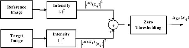
This threshold results in the target appearing in the final motion detection image only at the position it was occupying during acquisition of the second (test) data frame, since the target image at position corresponding to the first (reference) data frame appears as a negative value after intensity subtraction and is thus removed. It is noted that, unlike the complex amplitude image subtraction, there is no equivalent data domain representation for the intensity image subtraction or noncoherent CD approach due to the nonlinearity of the modulus function in (17.71). However, the delay line canceler framework can still be applied. The image intensity at each pixel can be viewed as a nonlinear function of the data in the respective frame, and the subtraction, implied by the DLC, is performed between two corresponding pixels separated by one or multiple frames.
The aforementioned change detection schemes, though presented for motion detection, can also be applied for detection of stationary targets in the presence of clutter and noise [89]. If a target-free background image of the scene being interrogated is available (feasible when the radar system is being used for long term surveillance), it can be subtracted (complex amplitude or intensity pixel subtraction) from an image of the same scene acquired at a later time that may contain a target of interest, thus rendering background subtraction as a special case of change detection.
2.17.4.3 Experimental results
A wideband through-the-wall imaging radar system was set up in the Radar Imaging Lab at Villanova University. A stepped-frequency CW signal, consisting of 101 frequency steps of size 10 MHz, covering 1.5–2.5 GHz band was chosen for imaging. The bandwidth of 1 GHz provides a range resolution of 15cm and the 10 MHz frequency step allows 15m unambiguous range, which is roughly three times the length of the room being imaged. An Agilent network analyzer, model ENA 5071B, was used for signal synthesis and data collection. A horn antenna, model ETS-Lindgren 3164-04, with an operational bandwidth from 0.7 to 6 GHz, was mounted on a Field Probe Scanner to synthesize an 11-element uniform receive line array with an inter-element spacing of 7.5cm. Two horn antennas (model ETS-Lindgren 3164-04), mounted on tripods and placed slightly above and on either side of the receive array, were used as transmitters. Each transmitter was spaced 3.75 cm away from the nearest receiver. Thus, for the system used, ![]() and
and ![]() . A 10 ft
. A 10 ft ![]() 8 ft wall segment was constructed utilizing 0.14 m thick solid concrete blocks with a dielectric constant of 7.66. The receive array was at a standoff distance of 1.05m from the wall, whereas the transmitters were positioned 1.33m in downrange from the wall.
8 ft wall segment was constructed utilizing 0.14 m thick solid concrete blocks with a dielectric constant of 7.66. The receive array was at a standoff distance of 1.05m from the wall, whereas the transmitters were positioned 1.33m in downrange from the wall.
In order to illustrate the performance of change detection under complex and intensity image delay line cancelers, we consider the following experiment. A human walks away from the front wall in an empty room, following a straight line path. Since simultaneous data cannot be collected at all receive locations due to the synthetic nature of the receive aperture, eight different target positions were considered, separated by 15 cm, along the trajectory, as illustrated in Figure 17.21. Data was collected for all eight positions, with the target stationary at each position, using time multiplexing of the transmitters. At each position, coherent integration was performed over 16 measurements. That is, ![]() for the experiment.
for the experiment.
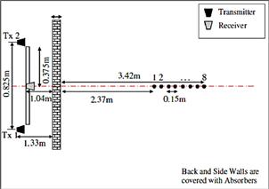
We first consider the case where the person moves from position 3 to position 4. That is, the two acquisitions are performed over consecutive frames and ![]() . Figure 17.22a and b show the beamformed images using the data corresponding to positions 3 and 4, respectively. Both images show strong reflections from the front wall, rendering target returns hard to detect in either image. Figure 17.23a shows the result of coherent change detection wherein the complex radar image of Figure 17.22a is subtracted from the complex image of Figure 17.22b. We observe that all stationary background including the front wall has been eliminated from the image, and the target undergoing motion has been detected. Since the target appears in two consecutive range cells, no clear target displacement is observed and the target image appears blurred. The corresponding noncoherent CD results under intensity image DLC are presented in Figure 17.23b. We observe that the intensity image DLC removes most of the imaged target in the case of consecutive range cell acquisitions. Moreover, due to the nonlinearity of the modulus function, the stationary background in the image is in general different for each data acquisition, thereby causing the background to be only partially canceled out under intensity image DLC [90]. As a result, stronger artifacts than those of the complex image DLC can be clearly observed. The ability to detect the target in the change detected image is, therefore, reduced under intensity image DLC as compared to complex image DLC.
. Figure 17.22a and b show the beamformed images using the data corresponding to positions 3 and 4, respectively. Both images show strong reflections from the front wall, rendering target returns hard to detect in either image. Figure 17.23a shows the result of coherent change detection wherein the complex radar image of Figure 17.22a is subtracted from the complex image of Figure 17.22b. We observe that all stationary background including the front wall has been eliminated from the image, and the target undergoing motion has been detected. Since the target appears in two consecutive range cells, no clear target displacement is observed and the target image appears blurred. The corresponding noncoherent CD results under intensity image DLC are presented in Figure 17.23b. We observe that the intensity image DLC removes most of the imaged target in the case of consecutive range cell acquisitions. Moreover, due to the nonlinearity of the modulus function, the stationary background in the image is in general different for each data acquisition, thereby causing the background to be only partially canceled out under intensity image DLC [90]. As a result, stronger artifacts than those of the complex image DLC can be clearly observed. The ability to detect the target in the change detected image is, therefore, reduced under intensity image DLC as compared to complex image DLC.
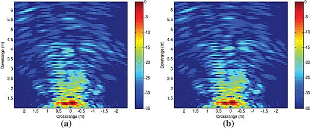
Figure 17.22 Beamformed images for the target at position (a) 3 and (b) 4 (consecutive range cells).

Figure 17.23 Images after change detection under (a) coherent CD and (b) noncoherent CD for the human walking from position 3 to position 4.
Next, we investigate the performance of the various schemes under large target displacement between consecutive acquisitions. Consider the case where the person moves from position 1 to position 4. In this case, ![]() . Figure 17.24a shows the result of coherent change detection. Since the target undergoes large range migration, the moving target presents itself as two targets in the image. The noncoherent change detection results for the large target displacement case are presented in Figure 17.24b. We observe that the intensity image DLC retains the target at position 4 and removes the target at position 1. However, similar to the small target displacement case, the artifacts resulting from the background not being totally canceled out render target detection difficult.
. Figure 17.24a shows the result of coherent change detection. Since the target undergoes large range migration, the moving target presents itself as two targets in the image. The noncoherent change detection results for the large target displacement case are presented in Figure 17.24b. We observe that the intensity image DLC retains the target at position 4 and removes the target at position 1. However, similar to the small target displacement case, the artifacts resulting from the background not being totally canceled out render target detection difficult.

2.17.5 Compressive sensing approach to moving target indication for urban sensing
The most desirable goal of a through-the-wall radar system is to provide situational awareness in a fast and reliable manner. This goal is primarily challenged due to increasing demands on the radar system to deliver high resolution images in both range and cross-range, which requires use of wideband signals and large array apertures, respectively. In addition, the presence of multipath and clutter can significantly contaminate the radar data and compromise the main intent of providing enhanced system capabilities for imaging of building interiors and tracking of targets behind walls.
Most radar data acquisition systems acquire samples in frequency (or time) and space, and then apply compression to reduce the amount of stored information. This approach has three inherent inefficiencies. First, as the demands for high resolution and more accurate information increase, so does the number of data samples to be recorded, stored, and subsequently processed. Second, there are significant data redundancies not exploited by the traditional sampling process. Third, it is wasteful to acquire and process data samples that will be discarded later. Further, in radar imaging systems, whether using time or stepped-frequency based pulsing, along data collection leads to image degradation. This is because, unless all objects in the scene are stationary during the entire data collection operations, image smearing of targets would occur.
Compressive sensing (CS) is a very effective technique for scene reconstruction from a relatively small number of data samples without compromising the imaging quality [94–98]. In general, the minimum number of data samples or sampling rate that is required for scene image formation is governed by the Nyquist theorem. However, when the scene is sparse, compressed sensing provides very efficient sampling, thereby significantly decreasing the required volume of data collected. Towards the objective of providing persistent surveillance in urban environments, such techniques will yield reduced cost, simplified hardware, and efficient sensing operations that allow super-resolution imaging of sparse behind-the-wall scenes. CS has been successfully applied to TWRI of moving and stationary targets [97,99].
In this section, we exploit full benefits of the compressive sensing to aid in fast data acquisition in wideband through-the-wall radar imaging systems for moving target detection and localization. Change detection is first used for removal of stationary background (clutter and stationary targets). Since the removal of stationary background via change detection converts a populated scene into a sparse scene of moving targets, reduction in data volume is then pursued under the framework of compressive sensing.
2.17.5.1 Signal model
Assume that there are N antenna locations constituting the synthetic aperture and a stepped-frequency signal of M narrowband signals. The signal received at the nth antenna location with the mth frequency is given by,
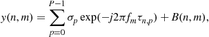 (17.73)
where ![]() is the reflection coefficient of the pth moving target,
is the reflection coefficient of the pth moving target, ![]() is the two-way propagation delay for the signal to travel from the nth antenna to the pth moving target, and
is the two-way propagation delay for the signal to travel from the nth antenna to the pth moving target, and ![]() represents the contribution of the stationary background. For free-space propagation,
represents the contribution of the stationary background. For free-space propagation, ![]() is proportional to the Cartesian distance between the nth antenna and the pth target, whereas in the presence of the wall, it contains contributions from paths in air and through the wall [100].
is proportional to the Cartesian distance between the nth antenna and the pth target, whereas in the presence of the wall, it contains contributions from paths in air and through the wall [100].
The MTI processing is achieved by collecting multiple data intervals over a period of time and buffering the corresponding stepped-frequency data measured at each antenna location [101]. Let I be the number of collected data intervals and ![]() , define the measured stepped-frequency dataset for the ith interval. It is noted that the timing interval for each dataset is a fraction of a second so that the moving target appears stationary during data collection. Change detection is applied to the measured datasets as follows,
, define the measured stepped-frequency dataset for the ith interval. It is noted that the timing interval for each dataset is a fraction of a second so that the moving target appears stationary during data collection. Change detection is applied to the measured datasets as follows,
![]() (17.74)
(17.74)
where ![]() , forming the set of difference signals
, forming the set of difference signals
![]() (17.75)
(17.75)
Using (17.73) and (17.74), the ith difference signal can be expressed as
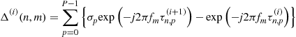 (17.76)
The component of the radar return from the stationary background is the same over the ith and (i + 1)th time intervals, and is thus removed from the difference signal. For moving targets, two situations may arise. In the first case, the target undergoes large range migration, whereas in the second case, the target undergoes small range migration, i.e., moves into the next range cell. In the first case, as seen from (17.76), the moving target will present itself as two targets, whereas in the second case, the target will appear as spread. We will focus on the former situation in this chapter.
2.17.5.2 Compressive sensing for MTI
Consider the ith difference dataset. For notational simplicity, we drop the superscript “(i).” Let ![]() be the
be the ![]() difference signal vector corresponding to the nth antenna location. For large range migration, an equivalent signal representation with
difference signal vector corresponding to the nth antenna location. For large range migration, an equivalent signal representation with ![]() targets can be used. Thus, with the region of interest divided into L pixels, the relationship between the difference signal
targets can be used. Thus, with the region of interest divided into L pixels, the relationship between the difference signal ![]() and the pixel locations can be expressed as [96,97]
and the pixel locations can be expressed as [96,97]
![]() (17.77)
(17.77)
where
 (17.78)
In (17.78), ![]() is the reflectivity of the qth target and
is the reflectivity of the qth target and ![]() is the two-way signal traveling time between the nth antenna location and lth pixel’s (qth target’s) location. The
is the two-way signal traveling time between the nth antenna location and lth pixel’s (qth target’s) location. The ![]() matrix is similar to the Fourier matrix which relates the frequency and time representations [97].
matrix is similar to the Fourier matrix which relates the frequency and time representations [97].
Given ![]() for
for ![]() , which is a
, which is a ![]() dimensional vector consisting of elements randomly chosen from
dimensional vector consisting of elements randomly chosen from ![]() , we can recover
, we can recover ![]() by solving the following equation:
by solving the following equation:
![]() (17.79)
(17.79)
where ![]() represents the tolerance error, and
represents the tolerance error, and
 (17.80)
In the above equation, ![]() and
and ![]() represent respective concatenations of
represent respective concatenations of ![]() and
and ![]() , and
, and ![]() for
for ![]() , are the indices of the randomly measured frequencies.
, are the indices of the randomly measured frequencies.
A stable solution of the sparse signal recovery problem in (17.79) is guaranteed provided that ![]() satisfies the Restricted Isometry Property (RIP), which states that all subsets of r columns taken from
satisfies the Restricted Isometry Property (RIP), which states that all subsets of r columns taken from ![]() are, in fact, nearly orthogonal, r being the sparsity of the signal
are, in fact, nearly orthogonal, r being the sparsity of the signal ![]() [102]. In practice, it is difficult to check this property. Other related measures on the matrix
[102]. In practice, it is difficult to check this property. Other related measures on the matrix ![]() , such as mutual coherence, are often used to guarantee stable recovery through
, such as mutual coherence, are often used to guarantee stable recovery through ![]() -minimization [102]. Mutual coherence of the columns of
-minimization [102]. Mutual coherence of the columns of ![]() can be viewed as the largest off-diagonal entry of the Gram matrix
can be viewed as the largest off-diagonal entry of the Gram matrix ![]() , where the columns of
, where the columns of ![]() have been normalized. The matrix
have been normalized. The matrix ![]() is considered to be incoherent if the value of the mutual coherence is small. For stepped-frequency systems, the coherence between the columns of
is considered to be incoherent if the value of the mutual coherence is small. For stepped-frequency systems, the coherence between the columns of ![]() is reduced by randomly distributing the selected frequency bins over the entire frequency band [96,97,103].
is reduced by randomly distributing the selected frequency bins over the entire frequency band [96,97,103].
Selecting a proper tolerance error ![]() is also very important for stable recovery of the scene being imaged. The tolerance error can be chosen using the cross-validation strategy [96,104], which does not require any knowledge or estimates of the noise statistics. This method depends on separating the data measurements into estimation and cross-validation sets. The CS method is applied to the estimation dataset with an initial selection of
is also very important for stable recovery of the scene being imaged. The tolerance error can be chosen using the cross-validation strategy [96,104], which does not require any knowledge or estimates of the noise statistics. This method depends on separating the data measurements into estimation and cross-validation sets. The CS method is applied to the estimation dataset with an initial selection of ![]() and the method’s result is tested on the cross-validation dataset. As the algorithm iterates, the prediction performance in the cross-validation set increases. When the method starts to overfit the estimation dataset, which means estimating part of the noise, performance in the cross-validation set decreases. Further decrease in
and the method’s result is tested on the cross-validation dataset. As the algorithm iterates, the prediction performance in the cross-validation set increases. When the method starts to overfit the estimation dataset, which means estimating part of the noise, performance in the cross-validation set decreases. Further decrease in ![]() is not beneficial and the algorithm should be terminated. The cross-validation based algorithm consists of the following steps, where the subscript “E” denotes the estimation set, and “CV” the cross-validation set:
is not beneficial and the algorithm should be terminated. The cross-validation based algorithm consists of the following steps, where the subscript “E” denotes the estimation set, and “CV” the cross-validation set:
ii. Estimate: Solve (17.79) to estimate the target locations ![]() with the estimation data set
with the estimation data set![]() .
.
iii. Cross-validate: If ![]() , then set
, then set ![]() , increment i and iterate from Step ii. Otherwise, terminate the iteration.
, increment i and iterate from Step ii. Otherwise, terminate the iteration.
Equations (17.79) and (17.80) represent one strategy that can be adopted for compressive sensing based MTI approach, wherein frequencies are chosen randomly for all the antenna locations constituting the array aperture. Figure 17.25a depicts the data collection scheme for the employed CS imaging strategy, wherein the horizontal axis is the frequency, the vertical axis represents the antenna position, and the dark boxes represent the sampled data. For comparison, the data collection scheme for conventional high-resolution radar is also provided in Figure 17.25b, which reiterates that all the frequency bins are transmitted and received at all antenna locations. Equations (17.79) and (17.80) can also be extended so that random measurements include both antennas and frequencies [96,97]. That is, a few frequency bins are collected at few antenna locations, as shown in Figure 17.25c.

2.17.5.3 Experimental results
A wideband SAR system was set up in the Radar Imaging Lab at Villanova University. A stepped-frequency CW signal, consisting of 201 frequency steps of size 10 MHz, covering 1–3 GHz band was chosen for imaging. An Agilent network analyzer, model ENA 5071B, was used for signal synthesis and data collection. A horn antenna, model ETS-Lindgren 3164-04, with an operational bandwidth from 0.7 to 6 GHz, was mounted on a Field Probe Scanner to synthesize a 41-element uniform linear array with an inter-element spacing of 3.745 cm, as shown in Figure 17.26a. A 3.05 m ![]() 2.44 m wall segment was constructed utilizing 0.14 m thick solid concrete blocks with a dielectric constant of 7.66. The array was at a standoff distance of 1.06 m from the wall. A 5 Gallon jug filled with salt water (emulating a human) was used as the target, as shown in Figure 17.26b. In order to emulate a moving target, two datasets were collected with the target at two different positions. Since simultaneous data cannot be collected at all antenna locations due to the synthetic nature of the array aperture, data were collected for the two positions, with the target stationary at each position. The target positions were selected as (0.8, 1.83) m and (0.25, 2.2) m, so as to emulate large range migration of the target between the two measurements.
2.44 m wall segment was constructed utilizing 0.14 m thick solid concrete blocks with a dielectric constant of 7.66. The array was at a standoff distance of 1.06 m from the wall. A 5 Gallon jug filled with salt water (emulating a human) was used as the target, as shown in Figure 17.26b. In order to emulate a moving target, two datasets were collected with the target at two different positions. Since simultaneous data cannot be collected at all antenna locations due to the synthetic nature of the array aperture, data were collected for the two positions, with the target stationary at each position. The target positions were selected as (0.8, 1.83) m and (0.25, 2.2) m, so as to emulate large range migration of the target between the two measurements.
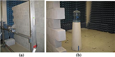
The region to be imaged is chosen to be 4.8 m ![]() 5.3 m centered in the middle of the scene beyond the wall and divided into 33
5.3 m centered in the middle of the scene beyond the wall and divided into 33 ![]() 57 pixels in crossrange and downrange. Figure 17.27a shows the result of change detection wherein the full dataset (201
57 pixels in crossrange and downrange. Figure 17.27a shows the result of change detection wherein the full dataset (201 ![]() 41 samples) corresponding to target position 1 is subtracted from that for position 2, followed by conventional image formation. We observe that all background returns have been eliminated from the image and the target undergoing motion has been detected. Moreover, as expected, the target has presented itself at the two locations corresponding to positions 1 and 2.
41 samples) corresponding to target position 1 is subtracted from that for position 2, followed by conventional image formation. We observe that all background returns have been eliminated from the image and the target undergoing motion has been detected. Moreover, as expected, the target has presented itself at the two locations corresponding to positions 1 and 2.

Figure 17.27 Change detection results using data from position 1 and position 2. (a) Beamforming with full difference dataset; (b) CS result with limited difference dataset; (c) beamforming with limited difference dataset.
For the CS approach, instead of measuring all 201 frequencies, we use a random subset of 7 frequencies only at each of the 41 antenna locations. According to CS theory, an r-sparse L-dimensional signal can be recovered from ![]() measurements [95]. Considering the system resolution and for the salt water jug extent of 0.27 m and 0.27 m in crossrange and downrange, respectively, each target will approximately occupy only 6 out of 1881 image pixels. For the large range migration case under consideration, the 41
measurements [95]. Considering the system resolution and for the salt water jug extent of 0.27 m and 0.27 m in crossrange and downrange, respectively, each target will approximately occupy only 6 out of 1881 image pixels. For the large range migration case under consideration, the 41 ![]() 7 measured data points well exceed this requirement ((2
7 measured data points well exceed this requirement ((2 ![]() 6) log (1881))
6) log (1881)) ![]() 90). The CS reconstructed image is shown in Figure 17.27b. For comparison, the beamformed image with the same reduced random dataset as CS is provided in Figure 17.27c. From Figure 17.27b, we observe that the CS approach localizes the target at positions 1 and 2 accurately. On the other hand, as seen in Figure 17.27c, beamforming with the reduced dataset has degraded image quality with significantly more false targets. A similar experiment without the absorbers on the side and back walls was conducted and shown to reduce the sparsity of the scene due to the presence of “ghosts.” The latter stems from the target-wall reflections and multipath returns. Compressive sensing can still be effective in localizing the target and its ghosts, but requires an increase in the number of data samples compared to the case of “no ghosts.”
90). The CS reconstructed image is shown in Figure 17.27b. For comparison, the beamformed image with the same reduced random dataset as CS is provided in Figure 17.27c. From Figure 17.27b, we observe that the CS approach localizes the target at positions 1 and 2 accurately. On the other hand, as seen in Figure 17.27c, beamforming with the reduced dataset has degraded image quality with significantly more false targets. A similar experiment without the absorbers on the side and back walls was conducted and shown to reduce the sparsity of the scene due to the presence of “ghosts.” The latter stems from the target-wall reflections and multipath returns. Compressive sensing can still be effective in localizing the target and its ghosts, but requires an increase in the number of data samples compared to the case of “no ghosts.”
2.17.6 Applications
Through-the-wall radar imaging has a variety of applications in both civil and military paradigms. It has been successfully sought out for surveillance and reconnaissance in urban environments, requiring not only the layout of the building, including types and locations of walls, but also detection and localization of both moving and stationary targets within enclosed structures [1,80,105]. This technology can also be used in rescue missions, searching for fire, earthquakes, and avalanche victims and survivors, behind-the-wall detection and surveillance of suspected criminals and outlaws, and by law enforcement officers for locating hostages and their captors [20,106].
2.17.7 Open issues and problems
There are many challenges still facing the TWRI technology. Imaging of stationary scenes using SAR is considered more difficult than MTI for moving targets. The difficulty arises from false positives and ghosts, both are products of multipath. Further, when targets are close to walls, imaging algorithms may not be able to separate targets from wall responses, as they both tend to merge. Another important TWRI goal is target classification. The relatively limited bandwidth does not lead to sufficient resolution of key scatterers, rendering the target image as a cluster of contagious high value pixels, a situation that does not lend itself to effective feature extraction. Classifications of Human gait take advantage of the motion of the limbs and their respective microDoppler signatures. When performed behind walls, these signatures blur and it can be difficult to achieve low classification errors. Complex buildings, made of multiple floors, each with populated scenes present the ultimate challenge of TWRI technology, specifically with long standoff distances whether it is associated with ground-based or airborne systems. The latter, due to covertness and operation logistics, is becoming the cornerstone of recent research and development in this area, especially for defense applications [107].
2.17.8 Data sets
The Center for Advanced Communications at Villanova University has conducted several through-the-wall imaging experiments and collected a variety of datasets in a laboratory environment. The datasets include full-polarization free-space and through-the-wall collections under semi-controlled conditions with a stepped-frequency radar system. Targets consist of both calibrated reflectors (dihedrals, trihedrals, and spheres) as well as a number of common indoor objects (phone, computer, tables, chair, filing cabinet). In addition, a jug of saline solution is also used as a target to crudely approximate a human. These datasets are available for download at the following website: http://www.villanova.edu/engineering/centers/cac/twri.htm .
2.17.9 Conclusion
In this chapter, we presented recent algorithmic advances in through-the-wall radar imaging. First, considering ground-based EM sensing, we discussed two methods, namely, spatial filtering and EM modeling based solution, for mitigating the front wall return prior to application of the image formation methods. The spatial filtering technique builds on the strong correlation of wall EM responses across antenna array elements to reduce constant-type return that is typical of walls in monostatic illuminations. The spatial filter, thus, allows the follow-on beamforming to unmask and image behind-the-wall targets that have limited spatial extent, such as humans, compared to walls without the need for a priori knowledge of the wall characteristics. A simple IIR notch filter with flexible design was compared with the fixed design MA subtraction filtering, commonly used in GPR. On the other hand, the EM modeling approach is wall-dependent and relies on accurate estimation of the wall parameters for suppression of the wall return. Extraction of the wall parameters and coherent subtraction of the modeled wall reflection was shown to significantly improve the signal-to- wall-clutter ratio.
Second, an approach to exploit the rich indoor multipath environment for improved target detection was described. A ray tracing approach was used to derive a multipath model, considering reflections inside an enclosed room comprising four homogeneous walls. Using the model, it was demonstrated analytically that the multipath corresponding to each sensor appeared on the wall but changes position from one sensor to another. Hence, a least squares technique was used to estimate its actual focusing location in both downrange and crossrange. The model was utilized to develop a multipath exploitation technique which associates multipath ghosts with their respective targets and maps them to their true target locations. This technique reduced the false positives in the original beamformed image as well as increased the signal-to-noise ratio at the true target locations.
Third, we discussed a change detection approach to moving target indication for through-the-wall applications. Change detection was used to mitigate the heavy clutter that is caused by strong reflections from exterior and interior walls. Both coherent and noncoherent change detection techniques were examined and their performance was compared under both consecutive and non-consecutive acquisitions. For non-consecutive acquisitions, the coherent CD scheme showed two sets of imaged targets corresponding to the positions of a single target at the two data acquisitions, whereas the noncoherent CD retained only one set of imaged targets, though with significantly more artifacts. For consecutive acquisitions, the coherent change detection provided better performance than the noncoherent CD, which removed most of the imaged target during the zero-thresholding step.
Finally, we identified and localized moving targets behind walls and inside enclosed structures using an approach that combines sparsity-driven radar imaging and moving target indication. The removal of stationary background via change detection resulted in a sparse scene of moving targets, thereby inviting application of compressed sensing techniques for fast data acquisition. Using stepped-frequency based radar imaging, it was demonstrated that a sizable reduction in the number of frequency samples was provided by compressive sensing without degradation in system performance.
Relevant Theory: Radar Signal Processing and Statistical Signal Processing
See this Volume, Chapter 10 Introduction: Radar Signal Processing
See Vol. 3, Chapter 6 Quickest Change Detection
References
1. Baranoski E. Through-wall imaging: historical perspective and future directions. J Franklin Inst. 2008;345(6):556–569.
2. Curlander JC, McDonough RN. Synthetic Aperture Radar-Systems and Signal Processing. New York: Wiley; 1991.
3. Goodman JW. Introduction to Fourier Optics. New York: McGraw-Hill; 1996.
4. Tyson RK. Principles of Adaptive Optics. second ed. Boston, MA: Academic Press; 1998; p. 1998.
5. Vaccaro RJ. The past, present, and the future of underwater acoustic signal processing. IEEE Signal Proc Mag. 1998;15(4):21–51.
6. Robinson EA, Treitel S. Geophysical Signal Analysis. Englewood Cliffs, NJ: Prentice-Hall; 1980.
7. Kak AC, Slaney M. Principles of Computerized Tomographic Imaging. New York: IEEE Press; 1988.
8. Ahmad F, Amin MG. Noncoherent approach to through-the-wall radar localization. IEEE Trans Aerosp Electron Syst. 2006;42(4):1405–1419.
9. Ahmad F, Amin MG. A noncoherent radar system approach for through-the-wall imaging. In: 2005;196–207. Proceedings of the SPIE—Sensors, and Command, Control, Communications, and Intelligence Technologies IV Conference, Orlando, FL. vol. 5778.
10. Ahmad F, Amin MG. Performance of autofocusing schemes for single target and populated scenes behind unknown walls. In: April 2007; Proceedings of the SPIE—Radar Sensor Technology XI, Orlando, FL. vol. 6547.
11. Ahmad F, Frazer G, Kassam SA, Amin MG. Design and implementation of near-field, wideband synthetic aperture beamformers. IEEE Trans Aerosp Electron Syst. 2004;40(1):206–220.
12. Ahmad F, Amin MG, Zemany PD. Performance analysis of dual-frequency CW radars for motion detection and ranging in urban sensing applications. In: April 2007; Proceedings of SPIE—Radar Sensor Technology XI, Orlando, FL. vol. 6547.
13. Amin MG, ed. Special Issue on Advances in Indoor Radar Imaging. J Franklin Inst. 2008;345(6):556–722.
14. Amin M, Sarabandi K, eds. Special Issue on Remote Sensing of Building Interior. IEEE Trans Geosci Remote Sens. 2009;47(5):1270–1420.
15. Borek SE. An overview of through the wall surveillance for homeland security. In: Proceedings of the 34th, Applied Imagery and Pattern Recognition Workshop. October 2005;19–21. 6.
16. Falconer DG, Ficklin RW, Konolige KG. Robot-mounted through-wall radar for detecting, locating, and identifying building occupants. In: Proceedings of the IEEE International Conference on Robotics and Automation. 2000;1868–1875.
17. Ferris Jr DD, Currie NC. A survey of current technologies for through-the-wall surveillance (TWS). In: November 1998;62–72. Proceedings of the SPIE—Sensors, C31 Information, and Training Technologies for Law Enforcement, Boston, MA. vol. 3577.
18. Fontana RJ. Recent system applications of short-pulse ultra-wideband (UWB) technology. in: IEEE Trans Microwave Theory Tech. 2004;52.
19. Frazier LM. Surveillance through walls and other opaque materials. In: Proceedings of the IEEE National Radar Conference 1996. 1996;27–31.
20. Greneker EF. RADAR flashlight for through-the-wall detection of humans. In: 1998;280–285. Proceedings of the SPIE—Targets Backgrounds: Characterization and Representation IV. vol. 3375.
21. Hunt AR. Image formation through walls using a distributed radar sensor network. In: 2005;169–174. Proceedings of the SPIE—Laser Physics, Photonics, Spectroscopy and Molecular Modeling V. vol. 5778.
22. Nag S, Barnes MA, Payment T, Holladay G. An ultra-wideband through-the-wall radar for detecting the motion of people in real time. In: April 2002;48–57. Proceedings of the SPIE—Radar Sensor Technology and Data Visualization, Orlando, FL. vol. 4744.
23. Song LP, Yu C, Liu QH. Through-wall imaging (TWI) by radar: 2-D tomographic results and analyses. IEEE Trans Geosci Remote Sens. 2005;43(12):2793–2798.
24. Soldovieri F, Solimene R. Through-wall imaging via a linear inverse scattering algorithm. IEEE Geosci Remote Sens Lett. 2007;4(4):513–517.
25. Soldovieri F, Ahmad F, Solimene R. Validation of microwave tomographic inverse scattering approach via through-the-wall experiments in semi-controlled conditions. IEEE Geosci Remote Sens Lett. 2011;8(1):123–127.
26. Frazier LM. Motion detection radar (MDR) for law enforcement. IEEE Potentials. 2004;16(5):3079–3082.
27. Ram SS, Ling H. Through-wall tracking of human movers using joint Doppler and array processing. IEEE Geosci Remote Sens Lett. 2008;5(3):537–541.
28. Setlur P, Ahmad F, Amin MG, Zemany PD. Experiments on through-the-wall motion detection and ranging. In: April 2007; Proceedings of the SPIE—Command, Control, Communications, and Intelligence (C3I) Technologies for Homeland Security and Homeland Defense VI, Orlando, FL. vol. 6538.
29. Setlur P, Amin MG, Thayaparan T. Micro-doppler signal estimation for vibrating and rotating targets. In: Proceedings of the Eighth International Symposium on Signal Processing and its Applications, Sydney, Australia. August 2005.
30. Thayaparan T, Stankovic L, Djurovic I. Micro-doppler human signature detection and its application to gait recognition and indoor imaging. J Franklin Inst. 2008;345(6):700–722.
31. Setlur P, Amin MG, Thayaparan T. Micro-doppler signal estimation for vibrating and rotating targets. In: Proceedings of the Eighth International Symposium on Signal Processing and its Applications, Sydney, Australia. August 2005.
32. Lai CP, Narayanan RM. Ultrawideband random noise radar design for through-wall surveillance. IEEE Trans Aerosp Electron Syst. 2010;46(4):1716–1730.
33. Lukin K, Konovalov V. Through wall detection and recognition of human beings using noise radar sensors. In: Proceedings of the NATO RTO SET Symposium on Target Identification and Recognition Using RF Systems, Oslo, Norway. October 2004;P15.1–P15.12.
34. T.E. McEwan, Ultra-Wideband Radar Motion Sensor, US Patent 5,361,070, 1994.
35. Venkatasubramanian V, Leung H. Chaos UWB radar for through-the-wall imaging. IEEE Trans Image Process. 2009;18(6):1255–1265.
36. Yang Y, Fathy AE. Development and implementation of a real-time see-through-wall radar system based on FPGA. IEEE Trans Geosci Remote Sens. 2009;47(5):1270–1280.
37. Ahmad F, Amin MG, Zemany PD. Dual-frequency radars for target localization in urban sensing. IEEE Trans Aerosp Electron Syst. 2009;45.
38. Ahmad F, Amin MG, Setlur P. Through-the-wall target localization using dual-frequency CW radars. In: April 2006; Proceedings of the SPIE—Sensors, and Command, Control, Communications, and Intelligence (C3I) Technologies Conference, Orlando, FL. vol. 6201.
39. Zhang Y, Amin MG, Ahmad F. Time-frequency analysis for the localization of multiple moving targets using dual-frequency radars. IEEE Signal Process Lett. 2008;15:777–780.
40. Ahmad F, Zhang Y, Amin M. Three-dimensional wideband beamforming for imaging through a single wall. IEEE Geosci Remote Sens Lett. 2008;5(2):176–179.
41. Ahmad F, Amin MG, Kassam SA. Synthetic aperture beamformer for imaging through a dielectric wall. IEEE Trans Aerosp Electron Syst. 2005;41(1):271–283.
42. Dehmollaian M, Thiel M, Sarabandi K. Through-the-wall imaging using differential SAR. IEEE Trans Geosci Remote Sens. 2009;47(5):1289–1296.
43. Ahmad F, Amin MG, Mandapati G. Autofocusing of through-the-wall radar imagery under unknown wall characteristics. IEEE Trans Image Process. 2007;16(7):1785–1795.
44. Dehmollaian M, Sarabandi K. Refocusing through building walls using synthetic aperture radar. IEEE Trans Geosci Remote Sens. 2008;46(6):1589–1599.
45. Yoon Y, Amin MG, Ahmad F. MVDR beamforming for through-the-wall radar imaging. IEEE Trans Aerosp Electron Syst. 2011;47(1):347–366.
46. G. Barrie, J. Tunaley, An Analysis of Through- and in-the-Wall UWB Impulse Radar: System Design Considerations, Technical Memorandum TM 2003-134, Defence Research and Development Canada (DRDC), 2003.
47. Komanduri VR, Hoorfar A, Engheta N. Low-profile array design considerations for through-the-wall microwave imaging applications. In: Proceedings of the IEEE International AP-S Symposium, Washington DC. July 2005.
48. Sévigny P, et al. Concept of operation and preliminary experimental results of the DRDC through-wall SAR system. In: April 2010; Proceedings of the SPIE—Radar Sensor Technology XIV, Orlando, FL. vol. 7669 pp. 766907-1–766907-11.
49. Greneker EF, Rausch EO. Wall characterization for through-the-wall radar applications. In: April 2008; Proceedings of the SPIE—Radar Sensor Technology XII Conference, Orlando, FL. vol. 6947.
50. Muqaibel A, Safaai-Jazi Ahmad. Characterization of wall dispersive and attenuative effects on UWB radar signals. J Franklin Inst. 2008;345:640–658.
51. Thajudeen C, Hoorfar A, Ahmad F, Dogaru T. Measured complex permittivity of walls with different hydration levels and the effect on power estimation of TWRI target returns. Prog Electromagn Res B. 2011;30:177–199.
52. Burkholder RJ. Electromagnetic models for exploiting multi-path propagation in through-wall radar imaging. In: Proceedings of the International Conference on Electromagnetics in Advanced Applications. Torino, Italy: IEEE; 2008;572–575.
53. Chang PC, Burkholder RJ, Volakis JL, Marhefka RJ, Bayram Y. High-frequency EM characterization of through-wall building imaging. IEEE Trans Geosci Remote Sens. 2009;47(5):1375–1387.
54. Dogaru T, Le C. SAR images of rooms and buildings based on FDTD computer models. IEEE Trans Geosci Remote Sens. 2009;47(5):1388–1401.
55. Thiel M, Sarabandi K. Ultrawideband multi-static scattering analysis of human movement within buildings for the purpose of stand-off detection and localization. IEEE Trans Antenn Propag. 2011;59(4):1261–1268.
56. Dehmollaian M, Sarabandi K. An approximate solution of scattering from reinforced concrete walls using an analytic 1-D periodic Green’s function. IEEE Trans Antenn Prop. 2008;56(8):2681–2690.
57. Solimene R, Ahmad F, Soldovieri F. A novel CS-SVD strategy to perform data reduction in linear inverse scattering problems. IEEE Geosci Remote Sens Lett. 2012;9(5):881–885.
58. T. Dogaru, C. Le, Through-the-Wall Small Weapon Detection Based on Polarimetric Radar Techniques, US ARL Technical Report ARL-TR-5041, Adelphi, MD, 2009.
59. Yemelyanov KM, Engheta N, Hoorfar A, McVay JA. Adaptive polarization contrast techniques for through-wall microwave imaging applications. IEEE Trans Geosci Remote Sens. 2009;47(5):1362–1374.
60. Zhang W, Hoorfar A, Thajudeen C, Ahmad F. Full polarimetric beamforming algorithm for through-the-wall radar imaging. Radio Sci. 2010;46. doi 10.1029/2010RS004631.
61. Tivive FHC, Bouzerdoum A, Amin MG. An SVD-based approach for mitigating wall reflections in through-the-wall radar imaging. In: Proceedings of the IEEE Radar Conference, Kansas City, MO. May 2011;519–524. 23–27.
62. Chandra R, Gaikwad AN, Singh D, Nigam MJ. An approach to remove the clutter and detect the target for ultra-wideband through wall imaging. J Geophys Eng. 2008;5(4):412–419.
63. Verma PK, Gaikwad AN, Singh D, Nigam MJ. Analysis of clutter reduction techniques for through wall imaging in UWB range. Prog Electromagn Res B. 2009;17:29–48.
64. Yoon Y-S, Amin MG. Spatial filtering for wall-clutter mitigation in through-the-wall radar imaging. IEEE Trans Geosci Remote Sens. 2009;47(9):3192–3208.
65. Brunzell H. Detection of shallowly buried objects using impulse radar. IEEE Trans Geosci Remote Sens. 1999;37(2):875–886.
66. Gustaffson F. Determining the initial states in forward-backward filtering. IEEE Trans Signal Process. 1996;44(4):988–992.
67. Çetin M, Karl W, Castañon D. Evaluation of a regularized SAR imaging technique based on recognition-oriented features. In: April 2000;40–51. Proceedings of the SPIE—Algorithms for SAR Imagery VII, Orlando, FL. vol. 4053.
68. Dehmollaian M, Sarabandi K. Analytical, numerical, and experimental methods for through-the-wall radar imaging. In: April 2008;5181–5184. Proceedings of the IEEE International Conference on Acoustics, Speech, and Signal Processing, Las Vegas, NV .
69. Kong JA. Electromagnetic Wave Theory. Cambridge, MA: EMW Publishing; 2000.
70. Thajudeen C, Hoorfar A. A Comparative study of wall parameter estimation and mitigation techniques. In: Proceedings of the USNC/URSI Meeting, Toronto, Canada. July 2010.
71. Zhang J, Huang Y. Extraction of dielectric properties of building materials from free-space time-domain measurement. In: September 1999;127–132. Proceedings of High Frequency Postgraduate Student Colloquium .
72. Ahmad F, Amin MG. Multi-location wideband synthetic aperture imaging for urban sensing applications. J Franklin Inst. 2008;345(6):618–639.
73. T. Dogaru, C. Le, Validation of Xpatch Computer Models for Human Body Radar Signature, US ARL Technical Report ARL-TR-4403, Adelphi, MD, 2008.
74. Kidera S, Sakamoto T, Sato T. Experimental study of shadow region imaging algorithm with multiple scattered waves for UWB radars. Prog Electromagn Res. 2009;5(4):393–396.
75. Alli G, DiFilippo D. Beamforming for through-the-wall radar imaging. In: Amin MG, ed. Through-the-Wall Radar Imaging. Boca Raton, FL: CRC Press; 2010;81–120.
76. Amin MG, Ahmad F. Wideband synthetic aperture beamforming for through-the-wall imaging. IEEE Signal Process Mag. 2008;25(4):110–113.
77. Setlur P, Amin MG, Ahmad F. Multipath model and exploitation in through-the-wall and urban radar sensing. IEEE Trans Geosci Remote Sens. 2011;49(10):4021–4034.
78. Yoon Y-S, Amin MG. High-resolution through-the-wall radar imaging using beamspace MUSIC. IEEE Trans Antenn Propag. 2008;56(6):1763–1774.
79. Wang G, Amin MG, Zhang Y. A new approach for target locations in the presence of wall ambiguity. IEEE Trans Aerosp and Electron Syst. 2006;42(1):301–315.
80. Amin MG, ed. Through-the-Wall Radar Imaging. Boca Raton, FL: CRC Press; 2010.
81. Lai CP, Narayanan RM. Through-wall imaging and characterization of human activity using ultrawideband (UWB) random noise radar. In: May 2005;186–195. Proceedings of the SPIE Sensors and C3I Technologies for Homeland Security and Homeland Defense, Orlando, FL. vol. 5778.
82. Martone A, Ranney K, Innocenti R. Through-the-wall detection of slow-moving personnel. In: April 13–17, 2009; Proceedings of the SPIERadar Sensor Technology XIII, Orlando, FL. vol. 7308 pp. 73080Q1–73080Q12.
83. Skolnik M. Introduction to Radar Systems. third ed. New York: McGraw Hill; 2001; p. 2001.
84. Narayanan RM, Shastry MC, Chen PH, Levi M. Through-the-wall detection of stationary human targets using Doppler radar. Prog Electromagn Res B. 2010;20:147–166.
85. Orovic I, Stankovic S, Amin M. A new approach for classification of human gait based on time-frequency feature representations. Signal Process. 2011;91(6):1448–1456.
86. Ram SS, Li Y, Lin A, Ling H. Doppler-based detection and tracking of humans in indoor environments. J Franklin Inst. 2008;345(6):679–699.
87. Tahmoush D, Silvious J. Stride rate in radar micro-doppler images. In: Proceedings of the IEEE International Conference on Systems, Man, and Cybernetics, San Antonio, TX. October 2009;4218–4223. 11–14.
88. Ranney K, et al. Recent MTI experiments using ARL’s synchronous impulse reconstruction (SIRE) radar. In: April 2008; Proceedings of the SPIE—Radar Sensor Technology XII, Orlando, FL. vol. 6947 pp. 694708-1–694708-9.
89. Moulton J, Kassam SA, Ahmad F, Amin MG, Yemelyanov K. Target and change detection in synthetic aperture radar sensing of urban structures. In: Proceedings of the IEEE Radar Conference, Rome, Italy. May 2008; 26–30.
90. Soldovieri F, Solimene R, Pierri R. A simple strategy to detect changes in through the wall imaging. Prog Electromagn Res. 2009;M7:1–13.
91. Hunt AR. Use of a frequency-hopping radar for imaging and motion detection through walls. IEEE Trans Geosci Remote Sens. 2009;47(5):1402–1408.
92. Zhang YD, Hunt A. Image and localization of behind-the-wall targets using collocated and distributed apertures. In: Amin MG, ed. Through-the-Wall Radar Imaging. Boca Raton, FL: CRC Press; 2010;121–156. (Chapter 4).
93. Maaref N, Millot P, Pichot C, Picon O. A study of UWB FM-CW Radar for the detection of human beings in motion inside a building. IEEE Trans Geosci Remote Sens. 2009;47(5):1297–1300.
94. Proceedings of SPIE vol. 8365. Compressive Sensing. Bellingham, WA: SPIE; 2012.
95. Candes E, Romberg J, Tao T. Stable signal recovery from incomplete and inaccurate measurements. Commun Pure Appl Math. 2006;59:1207–1223.
96. Gurbuz A, McClellan J, Scott W. A compressive sensing data acquisition and imaging method for stepped frequency GPR. IEEE Trans Signal Process. 2009;57(7):2640–2650.
97. Yoon Y-S, Amin MG. Compressed sensing technique for high-resolution radar imaging. In: April 2008; Proceedings of the SPIE, Orlando, FL. vol. 6968 pp. 69681A-1–69681A-10.
98. Donoho D, Elad M, Temlyakov V. Stable recovery of sparse overcomplete representations in the presence of noise. IEEE Trans Inform Theory. 2006;52(1):6–18.
99. F. Ahmad, M. Amin, Compressive urban sensing, SPIE Newsroom, Published Online: 27 September 2012, http://dx.doi.org/10.1117/2.1201209.004413, <http://spie.org/x90448.xml>, 2012.
100. Wang G, Amin MG. Imaging through unknown walls using different standoff distances. IEEE Trans Signal Process. 2006;54(10):4015–4025.
101. Martone A, Ranney K, Innocenti R. Automatic through the wall detection of moving targets using low-frequency ultra-wideband radar. In: May 2010;39–43. Proceedings of the IEEE International Radar Conference, Washington D.C. .
102. Potter LC, Ertin E, Parker JT, Cetin M. Sparsity and compressed sensing in radar imaging. Proc IEEE. 2010;98(6):1006–1020.
103. Huang Q, Qu L, Wu B, Fang G. UWB through-wall imaging based on compressive sensing. IEEE Trans Geosci Remote Sens. 2010;48(3):1408–1415.
104. Boufounos P, Duarte MF, Baraniuk RG. Sparse signal reconstruction from noisy compressive measurements using cross-validation. In: Proceedings of the 2007 IEEE 14th Workshop on Statistical, Signal Processing. 2007.
105. Farwell M, et al. Sense through the wall system development and design considerations. J Franklin Inst. 2008;345(6):570–591.
106. Pieraccini M, Luzi G, Dei D, Pieri L, Atzeni C. Detection of breathing and heartbeat through snow using a microwave transceiver. IEEE Geosci Remote Sens Lett. 2008;5(1):57–59.
107. Ertin E, Moses RL. Through-the-wall SAR attributed scattering center feature estimation. IEEE Trans Geosci Remote Sens. 2009;47(5):1338–1348.