
Distributed Detection and Estimation in Wireless Sensor Networks
Sergio Barbarossa, Stefania Sardellitti and Paolo Di Lorenzo, Department of Information Engineering, Electronics and Telecommunications, Sapienza University of Rome, Via Eudossiana 18, 00184 Rome, Italy
Abstract
Wireless sensor networks (WSNs) are becoming more and more a pervasive tool to monitor a wide range of physical phenomena. The opportunities arising from the many potential applications raise a series of technical challenges coupled with implementation constraints, such as energy supply, latency and vulnerability. The need for an efficient design of a WSN requires a strict interplay between the sensing and communication phases. In this article, we provide an overview of various distributed detection and estimation algorithms, incorporating the constraints imposed by the communication channel and the application requirements. We consider both cases where sensing is distributed, but the decision is centralized, and the case where the decision itself is totally decentralized. Specific attention is devoted to achieve globally optimal results through the interaction of nearby nodes only. We show how the topology of the network plays a significant role in the performance of the distributed algorithms, in terms of energy expenditure and latency. Then, we show how to optimize the network topology in order to minimize energy consumption or to match the graph describing the statistical dependencies among the variables observed by the nodes.
Keywords
Distributed detection; Distributed estimation; Wireless sensor networks
2.07.1 Introduction
Wireless sensor networks (WSN) are receiving a lot of attention from both the theoretical and application sides, in view of the many applications spanning from environmental monitoring, as a tool to control physical parameters such as temperature, vibration, pressure, or pollutant concentration, to the monitoring of civil infrastructures, such as roads, bridges, buildings, etc. [1]. Some new areas of applications are emerging rapidly and have great potentials. A field that is gaining more and more interest is the use of WSNs as a support for smart grids. In such a case, a WSN is useful to: (i) monitor and predict energy production from renewable sources of energy such as wind or solar energy; (ii) monitor energy consumption; (iii) detect anomalies in the network. A further area of increasing interest is vehicular sensor networks. In such a case, the vehicles are nodes of an ad hoc network. The sensors onboard the vehicle can measure speed and position of the vehicle and forward this information to nearby vehicles or to the road side units (RSU). This information enables the construction of dynamic spatial traffic maps, which can be exploited to reroute traffic in case of accidents or to minimize energy consumption. A relatively recent and interesting application of WSNs is cognitive radio![]() . In such a case, opportunistic (or secondary) users are allowed to access temporally unoccupied spectrum holes, under the constraint of not interfering with licensed (primary) users, and to release the channels as soon as they are requested by licensed users. The basic step enabling this dynamic access is sensing. The problem is that if sensing is carried out at a single location, it might be severely degraded by shadowing phenomena: If the sensor is in shadowed area, it might miss the presence of a primary user and then transmit by mistake over occupied slots, thus generating an undue interference. To overcome shadowing, it is useful to resort to a WSN whose nodes sense the channels and exchange information with each other in order to mitigate the effect of local shadowing phenomena. The goal of the WSN in such an application is to build a spatial map of channel occupancy. An opportunistic user willing to access radio resources within a confined region could then interrogate the closest sensor of a WSN and get a reliable information about which channels are temporarily availableand when this utilization has to be stopped. The plethora of applications raises a series of challenging technical issues, which may be seen as sources of opportunities for engineers. Probably the first most important question concerns energy supply. In many applications, in fact, the sensors are battery-operated and it may be difficult or costly to recharge the batteries or to substitute them. As a consequence, energy consumption is a basic constraint that should be properly taken into account. A second major concern is reliability of the whole system. In many cases, to allow for an economy of scale, the single sensors are devices with limited accuracy and computational capabilities. Nevertheless, the decision taken by the network as a whole must be very reliable, because it might affect crucial issues like security, safety, etc. The question is then how to build a reliable system out of the combination of many potentially unreliable nodes. Nature exhibits many examples of such systems. Human beings are capable of solving very sophisticated tasks and yet they are essentially built around basic unreliable chemical reactions occurring within cells whose lifetime is typically much smaller than the lifetime of a human being. Clearly, engineering is still far away from approaching the skills of living systems, but important inspirations can be gained by observing biological systems. Two particular features possessed by biological systems are self-organization and self-healing capabilities. Introducing these capabilities within a sensor network is the way to tackle the problem of building a reliable system out of the cooperation of many potentially unreliable units. In particular, self-organization is a key tool to enable the network to reconfigure itself, in terms of acquisition and transfer of information from the sensing nodes to the control centers, responsible for taking decisions, launching alarms or activating actuators aimed to counteract adverse phenomena. The network architecture plays a fundamental role in terms of reliability of the whole system. In conventional WSNs, there is typically one or a few sink nodes that collect the observations taken by the sensor nodes and process them, in a centralized fashion, to produce the desired decision about the observed phenomenon. This architecture arises a number of critical issues, such as: (a) potential congestion around the sink nodes; (b) vulnerability of the whole network to attacks or failure of sink nodes; (c) efficiency of the communication links established to send data from the sensor nodes to the sink. For all these reasons, a desirable characteristic of a WSN is to be designed in such a way that decisions are taken in a decentralized manner. Ideally, every node should be able, in principle, to achieve the final decision, thanks to the exchange of information with the other nodes, either directly or through multiple hops. In this way, vulnerability would be strongly reduced and the system would satisfy a scalability property. In practice, it is not necessary to make every single node to be able to take decisions as reliably as in a centralized system. But what is important to emphasize is that proper interaction among the nodes may help to improve reliability of single nodes, reduce vulnerability and congestion events, and make a better usage of radio resource capabilities. This last issue points indeed to one of the distinctive features of decentralized decision systems, namely the fact that sensing and communicating are strictly intertwined with each other and a proper system design must consider them jointly. The first important constraint inducing a strict link between sensing and communicating is that the transmission of the measurements collected by the nodes to the decision points occurs over realistic channels, utilizing standard communication protocols. For example, adopting common digital communication systems, the data gathered by the sensors need to be quantized and encoded before transmission. In principle, the number of bits used in each sensor should depend on the accuracy of the data acquisition on that sensor. At the same time, the number of bits transmitted per each channel use is upper bounded by the channel capacity, which depends on the transmit power and on the channel between sensor and sink node. This suggests that the number of bits to be used in each node for data quantization should be made dependent on both sensor accuracy and transmission channel. A further important consequence of the network architecture and of the resulting flow of information from peripheral sensing nodes to central decision nodes is the latency with which a global decision can be taken. In a centralized decision system, the flow of information proceeds from the sensing nodes to the central control nodes, usually through multiple hops. The control node collects all the data, it carries out the computations, and takes a decision. Conversely, in a decentralized decision system, there is typically an iterated exchange of data among the nodes. This determines an increase of the time necessary to reach a decision. Furthermore, an iterated exchange of data implies an iterated energy consumption. Since in WSNs energy consumption is a fundamental concern, all the means to minimize the overall energy consumption necessary to reach a decision within a maximum latency are welcome. At a very fundamental level, we will see how an efficient design of the network requires a global cross layer design where the physical and the routing layers take explicitly into account the specific application for which the network has been built.
. In such a case, opportunistic (or secondary) users are allowed to access temporally unoccupied spectrum holes, under the constraint of not interfering with licensed (primary) users, and to release the channels as soon as they are requested by licensed users. The basic step enabling this dynamic access is sensing. The problem is that if sensing is carried out at a single location, it might be severely degraded by shadowing phenomena: If the sensor is in shadowed area, it might miss the presence of a primary user and then transmit by mistake over occupied slots, thus generating an undue interference. To overcome shadowing, it is useful to resort to a WSN whose nodes sense the channels and exchange information with each other in order to mitigate the effect of local shadowing phenomena. The goal of the WSN in such an application is to build a spatial map of channel occupancy. An opportunistic user willing to access radio resources within a confined region could then interrogate the closest sensor of a WSN and get a reliable information about which channels are temporarily availableand when this utilization has to be stopped. The plethora of applications raises a series of challenging technical issues, which may be seen as sources of opportunities for engineers. Probably the first most important question concerns energy supply. In many applications, in fact, the sensors are battery-operated and it may be difficult or costly to recharge the batteries or to substitute them. As a consequence, energy consumption is a basic constraint that should be properly taken into account. A second major concern is reliability of the whole system. In many cases, to allow for an economy of scale, the single sensors are devices with limited accuracy and computational capabilities. Nevertheless, the decision taken by the network as a whole must be very reliable, because it might affect crucial issues like security, safety, etc. The question is then how to build a reliable system out of the combination of many potentially unreliable nodes. Nature exhibits many examples of such systems. Human beings are capable of solving very sophisticated tasks and yet they are essentially built around basic unreliable chemical reactions occurring within cells whose lifetime is typically much smaller than the lifetime of a human being. Clearly, engineering is still far away from approaching the skills of living systems, but important inspirations can be gained by observing biological systems. Two particular features possessed by biological systems are self-organization and self-healing capabilities. Introducing these capabilities within a sensor network is the way to tackle the problem of building a reliable system out of the cooperation of many potentially unreliable units. In particular, self-organization is a key tool to enable the network to reconfigure itself, in terms of acquisition and transfer of information from the sensing nodes to the control centers, responsible for taking decisions, launching alarms or activating actuators aimed to counteract adverse phenomena. The network architecture plays a fundamental role in terms of reliability of the whole system. In conventional WSNs, there is typically one or a few sink nodes that collect the observations taken by the sensor nodes and process them, in a centralized fashion, to produce the desired decision about the observed phenomenon. This architecture arises a number of critical issues, such as: (a) potential congestion around the sink nodes; (b) vulnerability of the whole network to attacks or failure of sink nodes; (c) efficiency of the communication links established to send data from the sensor nodes to the sink. For all these reasons, a desirable characteristic of a WSN is to be designed in such a way that decisions are taken in a decentralized manner. Ideally, every node should be able, in principle, to achieve the final decision, thanks to the exchange of information with the other nodes, either directly or through multiple hops. In this way, vulnerability would be strongly reduced and the system would satisfy a scalability property. In practice, it is not necessary to make every single node to be able to take decisions as reliably as in a centralized system. But what is important to emphasize is that proper interaction among the nodes may help to improve reliability of single nodes, reduce vulnerability and congestion events, and make a better usage of radio resource capabilities. This last issue points indeed to one of the distinctive features of decentralized decision systems, namely the fact that sensing and communicating are strictly intertwined with each other and a proper system design must consider them jointly. The first important constraint inducing a strict link between sensing and communicating is that the transmission of the measurements collected by the nodes to the decision points occurs over realistic channels, utilizing standard communication protocols. For example, adopting common digital communication systems, the data gathered by the sensors need to be quantized and encoded before transmission. In principle, the number of bits used in each sensor should depend on the accuracy of the data acquisition on that sensor. At the same time, the number of bits transmitted per each channel use is upper bounded by the channel capacity, which depends on the transmit power and on the channel between sensor and sink node. This suggests that the number of bits to be used in each node for data quantization should be made dependent on both sensor accuracy and transmission channel. A further important consequence of the network architecture and of the resulting flow of information from peripheral sensing nodes to central decision nodes is the latency with which a global decision can be taken. In a centralized decision system, the flow of information proceeds from the sensing nodes to the central control nodes, usually through multiple hops. The control node collects all the data, it carries out the computations, and takes a decision. Conversely, in a decentralized decision system, there is typically an iterated exchange of data among the nodes. This determines an increase of the time necessary to reach a decision. Furthermore, an iterated exchange of data implies an iterated energy consumption. Since in WSNs energy consumption is a fundamental concern, all the means to minimize the overall energy consumption necessary to reach a decision within a maximum latency are welcome. At a very fundamental level, we will see how an efficient design of the network requires a global cross layer design where the physical and the routing layers take explicitly into account the specific application for which the network has been built.
This chapter is organized as follows. In Section 2.07.2, we provide a general framework aimed to show how an efficient design of a sensor network requires a joint organization of in-network processing and communication. We show how the organization of the flow of information from the sensing nodes to the decision centers should depend not only on the WSN topology, but also on the statistical model of the observation. Finally, we briefly recall some fundamental information theoretical issues showing how in a multi-terminal decision network source and channel coding are strictly related to each other. In Section 2.07.3, we introduce the graph model as the formal tool to describe the interaction among the nodes. Then, we illustrate the so called consensus algorithm as a basic tool to reach globally optimal decisions through a decentralized approach. Since the interaction among the nodes occurs through a wireless channel, we also consider the impact of realistic channel models on consensus algorithm and show how consensus algorithms can be made robust against channel impairments. In Section 2.07.4, we address the distributed estimation problem. We show first an entirely decentralized approach, where observations and estimations are performed without the intervention of a fusion center. In such a case, we show how to achieve a globally optimal estimation through the local exchange of information among nearby nodes. Then, we consider the case where the estimation is performed at a decision center. In such a case, we show how to allocate quantization bits and transmit powers in the links between the sensing nodes and the fusion center, in order to accommodate the requirement on the maximum estimation variance, under a constraint on the global transmit power. In Section 2.07.5, we extend the approach to the detection problem. Also in this case, we consider the entirely distributed approach, where every node is enabled to achieve a globally optimal decision, and the case where the decision is taken at a central control node. In such a case, we show how to allocate coding bits and transmit power in order to maximize the detection probability, under constraints on the false alarm rate and the global transmit power. Then, in Section 2.07.6, we generalize consensus algorithms illustrating a distributed procedure that does not force all the nodes to reach a common value, as in consensus algorithms, but rather to converge to the projection of the overall observation vector onto a signal subspace. This algorithm is especially useful, for example, when it is required to smooth out the effect of noise, but without destroying valuable information present in the spatial variation of the useful signal. In wireless sensor networks, a special concern is energy consumption. We address this issue in Section 2.07.7, where we show how to optimize the network topology in order to minimize the energy necessary to achieve a global consensus. We show how to convert this, in principle, combinatorial problem, into a convex problem with minimal performance losses. Finally, in Section 2.07.8, we address the problem of matching the topology of the observation network to the graph describing the statistical dependencies among the observed variables. Finally, in Section 2.07.9, we draw some conclusions and we try to highlight some open problems and possible future developments.
2.07.2 General framework
The distinguishing feature of a decentralized detection or estimation system is that the measurements are gathered by a multiplicity of sensors dispersed over space, while the decision about what is being sensed is taken at one or a few fusion centers or sink nodes. The information gathered by the sensors has then to propagate from the peripheral nodes to the central control nodes. The challenge coming from this set-up is that in a WSN, information propagates through wireless channels, which are inherently broadcast, affected by fading and prone to interference. Installing a WSN requires then to set up a proper medium access control protocol (MAC) able to handle the communications among the nodes, in order to avoid interference and to ensure that the information reaches the final destination in a reliable manner. But what is decidedly specific of a WSN is that the sensing and communication aspects are strictly related to each other. In designing the MAC of a WSN, there are some fundamental aspects that distinguish a WSN from a typical telecommunication (TLC) network. The main difference stems from the analysis of goal and constraints of these two kinds of networks. A TLC network must make sure that every source packet reaches the final destination, perhaps through retransmission in case of errors or packet drop, irrespective of the packet content. In a WSN, what is really important is that the decision about what is being sensed be taken in the most reliable way, without necessarily implying the successful delivery of all source packets. Moreover, one of the major constraints in WSNs is energy consumption, because the nodes are typically battery operated and recharging the batteries is sometimes troublesome, especially when the nodes are installed in hard to reach places. Conversely, in a TLC network, energy provision is of course important, but it is not the central issue. At the same time, the trend in TLC networks is to support higher and higher data rates to accommodate for ever more demanding applications, while the data rates typically required in most WSNs are not so high. These considerations suggest that an efficient design of a WSN should take into account the application layer directly. This means, for example, that it is not really necessary that every packet sent by a sensor node reaches the final destination. What is important is only that the correct decision is taken in a reliable manner, possibly with low latency and low energy consumption. This enables data aggregation or in-network processing to avoid unnecessary data transmissions. It is then important to formulate this change of perspective in a formal way to envisage ad hoc information transmission and processing techniques.
2.07.2.1 Computing while communicating
In a very general setting, taking a decision based on the data collected by the sensors can be interpreted as computing a function of these data. Let us denote by ![]() , with
, with ![]() , the measurements collected by the ith node of the network, and by
, the measurements collected by the ith node of the network, and by ![]() the function to be computed. The straightforward approach for computing this function consists in sending all the measurements
the function to be computed. The straightforward approach for computing this function consists in sending all the measurements ![]() to a fusion center through a proper communication network and then implement the computation of
to a fusion center through a proper communication network and then implement the computation of ![]() at the fusion center. However, if
at the fusion center. However, if ![]() possesses a structure, it may be possible to take advantage of such a structure to better organize the flow of data from the sensing nodes to the fusion center. The idea of mingling computations and communications to make an efficient use of the radio resources, depending on the properties that the function
possesses a structure, it may be possible to take advantage of such a structure to better organize the flow of data from the sensing nodes to the fusion center. The idea of mingling computations and communications to make an efficient use of the radio resources, depending on the properties that the function ![]() might possess, was proposed in [2]. Here, we will first recall the main results of [2]. Then, we will show how the interplay between computation and communication will be further affected by the structure of the probabilistic model underlying the observations.
might possess, was proposed in [2]. Here, we will first recall the main results of [2]. Then, we will show how the interplay between computation and communication will be further affected by the structure of the probabilistic model underlying the observations.
To exploit the structure of the function ![]() to be computed, it is necessary to define some relevant structural properties. One important property is divisibility. Let
to be computed, it is necessary to define some relevant structural properties. One important property is divisibility. Let ![]() be a subset of
be a subset of ![]() and let
and let ![]() be a partition of
be a partition of ![]() . We denote by
. We denote by ![]() the vector composed by the set of measurements collected by the nodes whose indices belong to
the vector composed by the set of measurements collected by the nodes whose indices belong to ![]() . A function
. A function ![]() is said to be divisible if, for any
is said to be divisible if, for any ![]() and any partition
and any partition ![]() , there exists a function
, there exists a function ![]() such that
such that
![]() (7.1)
(7.1)
In words, (7.1) represents a sort of “divide and conquer” property: A function ![]() is divisible if it is possible to split its computation into partial computations over subsets of data and then recombine the partial results to yield the desired outcome.
is divisible if it is possible to split its computation into partial computations over subsets of data and then recombine the partial results to yield the desired outcome.
Let us suppose now that the N sensing nodes are randomly distributed over a circle of radius R. We assume a simple propagation model, such that two nodes are able to send information to each other in a reliable way if their distance is less than a coverage radius ![]() . At the same time, the interference between two links is considered negligible if the interfering transmitter is at a distance greater than
. At the same time, the interference between two links is considered negligible if the interfering transmitter is at a distance greater than ![]() from the receiver, where
from the receiver, where ![]() is chosen according to the propagation model. For any random deployment of the nodes, the choice of
is chosen according to the propagation model. For any random deployment of the nodes, the choice of ![]() induces a network topology, such that there is a link between two nodes if their distance is less than
induces a network topology, such that there is a link between two nodes if their distance is less than ![]() . The resulting graph having the nodes as vertices and the edges as links, is a random graph, because the positions of the nodes are random. This kind of graph is known as a Random Geometric Graph (RGG).1 To make an efficient use of the radio resources, it is useful to take
. The resulting graph having the nodes as vertices and the edges as links, is a random graph, because the positions of the nodes are random. This kind of graph is known as a Random Geometric Graph (RGG).1 To make an efficient use of the radio resources, it is useful to take ![]() as small as possible, to save local transmit power and make possible the reuse of radio resources, either frequency or time slots. However,
as small as possible, to save local transmit power and make possible the reuse of radio resources, either frequency or time slots. However, ![]() should not be too small to loose connectivity. In other words, we do not want the network to split in subnetworks that do not interact with each other. Since the node location is random, network connectivity can only be guaranteed in probability. It has been proved in [3] that, if
should not be too small to loose connectivity. In other words, we do not want the network to split in subnetworks that do not interact with each other. Since the node location is random, network connectivity can only be guaranteed in probability. It has been proved in [3] that, if ![]() is chosen as follows:
is chosen as follows:
![]() (7.2)
(7.2)
with ![]() going to infinity, as N goes to infinity, the resulting RGG is asymptotically connected with high probability, as N goes to infinity. For instance, if we take
going to infinity, as N goes to infinity, the resulting RGG is asymptotically connected with high probability, as N goes to infinity. For instance, if we take ![]() , the coverage radius can be expressed simply as
, the coverage radius can be expressed simply as
![]() (7.3)
(7.3)
A further property of a node is the number of neighbors of that node. For an undirected graph, the number of neighbors of a node is known as the degree of the node. Denoting by ![]() the degree of an RGG with N nodes, it was proved in [4] that, choosing the coverage radius as in (7.2),
the degree of an RGG with N nodes, it was proved in [4] that, choosing the coverage radius as in (7.2), ![]() is (asymptotically) upper bounded by a function that behaves as
is (asymptotically) upper bounded by a function that behaves as ![]() . More specifically,
. More specifically,
![]() (7.4)
(7.4)
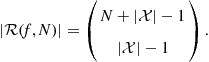
In [4] it was established an interesting link between the properties of the function ![]() to be computed by the network and the topology of the communication network. In particular, assuming as usual that the measurements are quantized in order to produce a value belonging to a finite alphabet, let us denote by
to be computed by the network and the topology of the communication network. In particular, assuming as usual that the measurements are quantized in order to produce a value belonging to a finite alphabet, let us denote by ![]() the range of
the range of ![]() and by
and by ![]() the cardinality of
the cardinality of ![]() . In [4], it was proved that, under the following assumptions:
. In [4], it was proved that, under the following assumptions:
then, the rate for computing ![]() scales with N as
scales with N as
![]() (7.5)
(7.5)
This is an important result that has practical consequences. It states, in fact, that, whenever ![]() scales with a law that increases more slowly than N, we can have an increase of efficiency if we organize the local computation and the flow of partial results properly. For instance, if the sensors communicate to the sink node through a Time Division Multiplexing Access (TDMA) scheme, with a standard approach it is necessary to allocate N time slots to send all the data to the sink node. Conversely, Eq. (7.5) suggests that, to compute the function
scales with a law that increases more slowly than N, we can have an increase of efficiency if we organize the local computation and the flow of partial results properly. For instance, if the sensors communicate to the sink node through a Time Division Multiplexing Access (TDMA) scheme, with a standard approach it is necessary to allocate N time slots to send all the data to the sink node. Conversely, Eq. (7.5) suggests that, to compute the function ![]() , it is sufficient to allocate
, it is sufficient to allocate ![]() slots. The same result would apply in a Frequency Division Multiplexing Access (FDMA) scheme, simply reverting the role of time slots and frequency subchannels. This is indeed a paradigm shift, because it suggests that an efficient radio resource allocation in a WSN should depend on the cardinality of
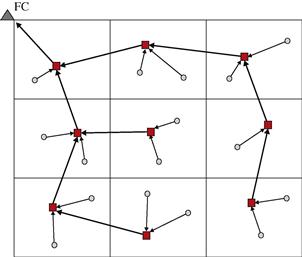
slots. The same result would apply in a Frequency Division Multiplexing Access (FDMA) scheme, simply reverting the role of time slots and frequency subchannels. This is indeed a paradigm shift, because it suggests that an efficient radio resource allocation in a WSN should depend on the cardinality of ![]() . This implies a sort of cross-layer approach that involves physical, MAC and application layers jointly. The next question is how to devise an access protocol that enables such an efficient design. To this regard, the theorem proved in [4] contains a constructive proof, which suggests how to organize the flow of information from the sensing nodes to the control center. In particular, the strategy consists in making a tessellation of the area monitored by the sensor network, similarly to a cellular network, as pictorially described in Figure 7.1. Furthermore, the information flows from the peripheral nodes to the fusion center through a tree-like graph, having the fusion center as its root. In each cell, the nodes (circles) identify a node as the relay node (square). The relay node collects data from the nodes within its own cell and from relay nodes of its leaves, performs local computations and communicates the result to the parent relay nodes, with the goal of propagating these partial results towards the root (sink node). To handle interference, a graph coloring scheme is used to avoid interference among adjacent cells. This allows spatial reuse of radio resources, e.g., frequency or time slots, which can be used in parallel without generating an appreciable interference. The communication structure is conceptually similar to a cellular network, with the important difference that now the flow of information is directly related to the computational task. A few examples are useful to better grasp the possibilities of this approach.
. This implies a sort of cross-layer approach that involves physical, MAC and application layers jointly. The next question is how to devise an access protocol that enables such an efficient design. To this regard, the theorem proved in [4] contains a constructive proof, which suggests how to organize the flow of information from the sensing nodes to the control center. In particular, the strategy consists in making a tessellation of the area monitored by the sensor network, similarly to a cellular network, as pictorially described in Figure 7.1. Furthermore, the information flows from the peripheral nodes to the fusion center through a tree-like graph, having the fusion center as its root. In each cell, the nodes (circles) identify a node as the relay node (square). The relay node collects data from the nodes within its own cell and from relay nodes of its leaves, performs local computations and communicates the result to the parent relay nodes, with the goal of propagating these partial results towards the root (sink node). To handle interference, a graph coloring scheme is used to avoid interference among adjacent cells. This allows spatial reuse of radio resources, e.g., frequency or time slots, which can be used in parallel without generating an appreciable interference. The communication structure is conceptually similar to a cellular network, with the important difference that now the flow of information is directly related to the computational task. A few examples are useful to better grasp the possibilities of this approach.
Data uploading: Suppose it is necessary to convey all the data to the sink node. If each observed vector belongs to an alphabet ![]() , with cardinality
, with cardinality ![]() , the cardinality of the whole data set is
, the cardinality of the whole data set is ![]() . Hence,
. Hence, ![]() . This means that, according to (7.5), the capacity of the network scales as
. This means that, according to (7.5), the capacity of the network scales as ![]() . This is a rather disappointing result, as it shows that there is no real benefit with respect to the simplest communication case one could envisage: The nodes have to split the available bandwidth into a number of sub-bands equal to the number of nodes, with a consequent rate reduction per node.
. This is a rather disappointing result, as it shows that there is no real benefit with respect to the simplest communication case one could envisage: The nodes have to split the available bandwidth into a number of sub-bands equal to the number of nodes, with a consequent rate reduction per node.
Decision based on the histogram of the measurements: Let us suppose now that the decision to be taken at the control node can be based on the histogram of the data collected by the nodes, with no information loss. In this case, the function ![]() is the histogram. It can be verified that the histogram is a divisible function. Furthermore, the cardinality of the histogram is
is the histogram. It can be verified that the histogram is a divisible function. Furthermore, the cardinality of the histogram is
 (7.6)
(7.6)
Furthermore, it can be shown that
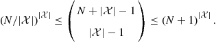 (7.7)
(7.7)
Hence, in this case ![]() behaves as
behaves as ![]() and then the rate
and then the rate ![]() in (7.5) scales as
in (7.5) scales as ![]() . This is indeed an interesting result, showing that if the decision can be based on the histogram of the data, rather than on each single measurement, adopting the right communication scheme, the rate per node behaves as
. This is indeed an interesting result, showing that if the decision can be based on the histogram of the data, rather than on each single measurement, adopting the right communication scheme, the rate per node behaves as ![]() , rather than
, rather than ![]() , with a rate gain
, with a rate gain ![]() , which increases as the number of nodes increases.
, which increases as the number of nodes increases.
Symmetric functions: Let us consider now the case where ![]() is a symmetric function. We recall that a function
is a symmetric function. We recall that a function ![]() is symmetric if it is invariant to permutations of its arguments, i.e.,
is symmetric if it is invariant to permutations of its arguments, i.e., ![]() for any permutation matrix
for any permutation matrix ![]() and any argument vector
and any argument vector ![]() . This property reflects the so called data-centric view, where what it important is the measurement per se, and not which node has taken which measurement. Examples of symmetric functions include the mean, median, maximum/minimum, histogram, and so on. The key property of symmetric functions is that it can be shown that they depend on the argument
. This property reflects the so called data-centric view, where what it important is the measurement per se, and not which node has taken which measurement. Examples of symmetric functions include the mean, median, maximum/minimum, histogram, and so on. The key property of symmetric functions is that it can be shown that they depend on the argument ![]() only through the histogram of
only through the histogram of ![]() . Hence, the computation of symmetric functions is a particular case of the example examined before. Thus, the rate scales again as
. Hence, the computation of symmetric functions is a particular case of the example examined before. Thus, the rate scales again as ![]() .
.
2.07.2.2 Impact of observation model
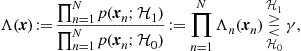
Having recalled that the efficient design of a WSN requires an information flow that depends on the scope of the network, more specifically, on the structural properties of the function to be computed by the network, it is now time to be more specific on the decision tasks that are typical of WSNs, namely detection and estimation. Let us consider for example the simple hypothesis testing problem. In such a case, an ideal centralized detector having error-free access to the measurements collected by the nodes, should compute the likelihood ratio and compare it with a suitable threshold [5]. We denote with ![]() and
and ![]() the two alternative hypotheses, i.e., absence or presence of the event of interest, and with
the two alternative hypotheses, i.e., absence or presence of the event of interest, and with ![]() the set of measurements collected by node i. If we indicate with
the set of measurements collected by node i. If we indicate with ![]() the joint probability density function of the whole set of observed data, under the hypothesis
the joint probability density function of the whole set of observed data, under the hypothesis ![]() , with
, with ![]() , the likelihood ratio test amounts to comparing the likelihood ratio (LR) with a threshold
, the likelihood ratio test amounts to comparing the likelihood ratio (LR) with a threshold ![]() , and decide for
, and decide for ![]() if the threshold is exceeded or for
if the threshold is exceeded or for ![]() , otherwise. In formulas
, otherwise. In formulas
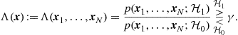 (7.8)
(7.8)
The LR test (LRT) is optimal under a Bayes or a Neyman-Pearson criterion, the only difference being that the threshold ![]() assumes different values in the two cases [5]. In principle, to implement the LRT at the fusion center, every node should send its observation vector
assumes different values in the two cases [5]. In principle, to implement the LRT at the fusion center, every node should send its observation vector ![]() to the fusion center, through a proper MAC protocol. The fusion center, after having collected all the data, should then implement the LRT, as indicated in (7.8). However, the computation of the LR in (7.8) does not necessarily imply the transmission of the single vectors
to the fusion center, through a proper MAC protocol. The fusion center, after having collected all the data, should then implement the LRT, as indicated in (7.8). However, the computation of the LR in (7.8) does not necessarily imply the transmission of the single vectors ![]() . Conversely, according to the theory recalled above, the transmission strategy should depend on the structural properties of the LR function, if any. Let us see how to exploit the structure of the LR function in two cases of practical interest.
. Conversely, according to the theory recalled above, the transmission strategy should depend on the structural properties of the LR function, if any. Let us see how to exploit the structure of the LR function in two cases of practical interest.
2.07.2.2.1 Statistically independent observations
Let us start assuming that the observations taken by different sensors are statistically independent, conditioned to each hypothesis. This is an assumption valid in many cases. Under such an assumption, the LR can be factorized as follows
 (7.9)
(7.9)
where ![]() denotes the local LR at the nth node. In this case, the global function
denotes the local LR at the nth node. In this case, the global function ![]() in (7.9) possesses a clear structure: It is factorizable in the product of the local LR functions. Then, since a factorizable function is divisible, it is possible to implement the efficient mechanisms described in the previous section to achieve an efficient design. The network nodes should cluster as in Figure 7.1. Every relay node should compute the local LR, multiply it to the data received from the relays pertaining to the lower clusters and send the partial result to the relay of the upper cluster, until the result reaches the fusion center. The efficiency comes from the fact that many transmissions can occur in parallel, exploiting spatial reuse of radio resources. This result suggests also that the proper source encoding to be implemented at each sensor node consists in the computation of the local LR.
in (7.9) possesses a clear structure: It is factorizable in the product of the local LR functions. Then, since a factorizable function is divisible, it is possible to implement the efficient mechanisms described in the previous section to achieve an efficient design. The network nodes should cluster as in Figure 7.1. Every relay node should compute the local LR, multiply it to the data received from the relays pertaining to the lower clusters and send the partial result to the relay of the upper cluster, until the result reaches the fusion center. The efficiency comes from the fact that many transmissions can occur in parallel, exploiting spatial reuse of radio resources. This result suggests also that the proper source encoding to be implemented at each sensor node consists in the computation of the local LR.
2.07.2.2.2 Markov observations
The previous result is appealing, but it pertains to the simple situation where the observations are statistically independent, conditioned to the hypotheses. In some circumstances, however, this assumption is unjustified. This is the case, for example, when the sensors monitor a field of spatially correlated values, like a temperature or atmospheric pressure field. In such cases, nearby nodes sense correlated values and then the statistical independence assumption is no longer valid. It is then of interest, in such cases, to check whether the statistical properties of the observations can still induce a structure on the function to be computed that can be exploited to improve network efficiency.
There is indeed a broad class of observation models where the joint pdf cannot be factorized into the product of the individual pdf’s pertaining to each node, but it can still be factorized into functions of subsets of variables. This is the case of Bayes networks or Markov random fields. Here we will recall the basic properties of these models, as relevant to our problem. The interested reader can refer to many excellent books, like, for example, [6] or [7].
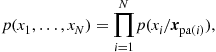
In the Bayes network’s case, the statistical dependency among the random variables is described by an acyclic directed graph, whose vertices represent the random variables, while the edges represent local conditional probabilities. In particular, given a node ![]() , whose parent nodes are identified by the set of indices
, whose parent nodes are identified by the set of indices ![]() , the joint probability density function (pdf) of a Bayes network can be written as
, the joint probability density function (pdf) of a Bayes network can be written as
 (7.10)
where ![]() collects all the variables corresponding to the parents of node i. If a node in (7.10) does not have parents, the corresponding probability is unconditional.
collects all the variables corresponding to the parents of node i. If a node in (7.10) does not have parents, the corresponding probability is unconditional.
Alternatively, a Markov random field is represented through an undirected graph. More specifically, a Markov network consists of:
1. An undirected graph ![]() , where each vertex
, where each vertex ![]() represents a random variable and each edge
represents a random variable and each edge ![]() represents statistical dependency between the random variables u and v;
represents statistical dependency between the random variables u and v;
2. A set of potential (or compatibility) functions ![]() (also called clique potentials), that associate a non-negative number to the cliques2 of G.
(also called clique potentials), that associate a non-negative number to the cliques2 of G.
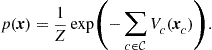
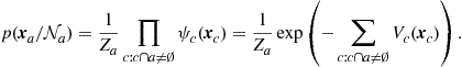
Let us denote by ![]() the set of all cliques present in the graph. The random vector
the set of all cliques present in the graph. The random vector ![]() is Markovian if its joint pdf admits the following factorization
is Markovian if its joint pdf admits the following factorization
![]() (7.11)
(7.11)
where ![]() denotes the vector of variables belonging to the clique c. The functions
denotes the vector of variables belonging to the clique c. The functions ![]() are called compatibility functions. The term Z is simply a normalization factor necessary to guarantee that
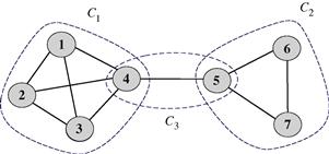
are called compatibility functions. The term Z is simply a normalization factor necessary to guarantee that ![]() is a valid pdf. A node p is conditionally independent of another node q in the Markov network, given some set S of nodes, if every path from p to q passes through a node in S. Hence, representing a set of random variables by drawing the correspondent Markov graph is a meaningful pictorial way to identify the conditional dependencies occurring across the random variables. As an example, let us consider the graph reported in Figure 7.2. The graph represents conditional independencies among seven random variables. The variables are grouped into 3 cliques. In this case, for example, we can say that nodes 1–4 are statistically independent of nodes 6 and 7, conditioned to the knowledge of node 5. In this example, the joint pdf can be written as follows
is a valid pdf. A node p is conditionally independent of another node q in the Markov network, given some set S of nodes, if every path from p to q passes through a node in S. Hence, representing a set of random variables by drawing the correspondent Markov graph is a meaningful pictorial way to identify the conditional dependencies occurring across the random variables. As an example, let us consider the graph reported in Figure 7.2. The graph represents conditional independencies among seven random variables. The variables are grouped into 3 cliques. In this case, for example, we can say that nodes 1–4 are statistically independent of nodes 6 and 7, conditioned to the knowledge of node 5. In this example, the joint pdf can be written as follows
![]() (7.12)
(7.12)
If the product in (7.11) is strictly positive for any ![]() , we can introduce the functions
, we can introduce the functions
![]() (7.13)
(7.13)
so that (7.11) can be rewritten in exponential form as
 (7.14)
This distribution is known, in physics, as the Gibbs (or Boltzman) distribution with interaction potentials![]() and energy
and energy![]() .
.
The independence graph conveys the key probabilistic information through absent edges: If nodes i and j are not neighbors, the random variables ![]() and
and ![]() are statistically independent, conditioned to the other variables. This is the so called pairwise Markov property. Given a subset
are statistically independent, conditioned to the other variables. This is the so called pairwise Markov property. Given a subset ![]() of vertices,
of vertices, ![]() factorizes as
factorizes as
![]() (7.15)
(7.15)
where the second factor does not depend on a. As a consequence, denoting by ![]() the set of all nodes except the nodes in a and by
the set of all nodes except the nodes in a and by ![]() the set of neighbors of the nodes in a,
the set of neighbors of the nodes in a, ![]() reduces to
reduces to ![]() . Furthermore,
. Furthermore,
 (7.16)
This property states that the joint pdf factorizes in terms that contain only variables whose vertices are neighbors.
An important example of jointly Markov random variables is the Gaussian Markov Random Field (GMRF), characterized by having a pdf expressed as in (7.14), with the additional property that the energy function is a quadratic function of the variables. In particular, a vector ![]() of random variables is a GMRF if its joint pdf can be written as
of random variables is a GMRF if its joint pdf can be written as
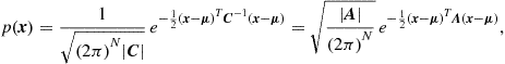 (7.17)
where ![]() is the expected value of
is the expected value of ![]() ,
, ![]() is the covariance matrix of
is the covariance matrix of ![]() and
and ![]() is the so called precision matrix. In this case, the Markovianity of
is the so called precision matrix. In this case, the Markovianity of ![]() manifests itself through the sparsity of the precision matrix. As a particular case of (7.16), the coefficient
manifests itself through the sparsity of the precision matrix. As a particular case of (7.16), the coefficient ![]() of
of ![]() is different from zero if and only if nodes i and j are neighbors.
is different from zero if and only if nodes i and j are neighbors.
Having recalled the main properties of GMRF’s, let us now go back to the problem of organizing the flow of information in a WSN aimed at deciding between two alternative hypotheses of GMRF. Let us consider for example the decision about the two alternative hypotheses:
![]() (7.18)
(7.18)
![]() (7.19)
(7.19)
where the sets of cliques involved in the two cases are, in general, different. The factorizations in (7.18, 7.19) suggest how to implement the computation of the LRT:
1. Each cluster in the WSN should be composed of the nodes associated to the random variables pertaining to the same clique in the statistical dependency graph;
2. The observations gathered by the nodes pertaining to a clique c are locally encoded into the clique potential ![]() . This is the value that has to be transmitted by each cluster towards upper layers or to the FC;
. This is the value that has to be transmitted by each cluster towards upper layers or to the FC;
3. As in Figure 7.1, each relay in the lowest layer compute the local potentials and forward these results to the upper layers. The relays of the intermediate clusters receive the partial results from the lower clusters, multiply these values by the local potential and forward the results to the relay of the upper cluster, until reaching the FC.
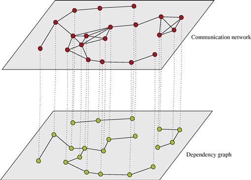
In general, different grouping may occur depending on the hypothesis. This organization represents a generalization of the distributed computation observed in the conditionally independent case, where the groups are simply singletons, i.e., sets composed by exactly one element. In that case, the clustering among nodes is only instrumental to the communication purposes, i.e., to enable spatial reuse of radio resources. In the more general Markovian case, the organization of the communication network in clusters (cells) should take into account, jointly, the grouping suggested by the cliques of the underlying dependency graph and the spatial grouping of nodes to enable concurrent transmission over the same radio resources without incurring in undesired interference. To visualize this general perspective, it is useful to have in mind two superimposed graphs, as depicted in Figure 7.3: the communication graph (top), whose vertices are the network nodes while the edges are the radio links; the dependency graph (bottom), whose vertices represent random variables, while the arcs represent statistical dependencies. Each communication cluster should incorporate at least one clique. Furthermore, in each cluster there is a relay node that is responsible for the exchange of data with nearby clusters. The whole communication network has a hierarchical tree-structure. Each node in the tree is a relay node belonging to a cluster. This node collects the measurements from the nodes belonging to its cluster, computes the potential (or the product of potentials if more cliques belong to the same cluster) and forwards this value to its relay parents. While we have depicted the two graphs as superimposed in Figure 7.3, it is useful to clarify that the nodes of the communication network are located in space and their relative position is well defined in a metric space. Conversely, the nodes of the Markov graph represent random variables for which there is no well defined notion of distance or, even if we define one, it is a notion that in general does not have a correspondence with distance in space. In other words, while the neighborhood of nodes in the top graph has to do with the concept of spatial distance among the nodes, the neighborhood of the nodes in the Markov graph has only to do with statistical dependencies. Nevertheless, it is also true that in the observation of physical entities like a temperature field, for example, it is reasonable to expect higher correlation among nearby (in the spatial sense) nodes (variables). An example of GMRF where the statistical dependencies incorporate the spatial distances was suggested in [8]. In summary, the previous considerations suggest that an efficient design of the communication network topology should keep into account the structure, if any, of dependency graph describing the observed variables. At the same time, the design of the network topology should keep into account physical constraints like the power consumption necessary to maintain the links with sufficient reliability (i.e., to insure the sufficient signal-to-noise ratio at the receiver). This is indeed an interesting line of research: How to match the network topology to the dependency graph, under physical constraints dictated by energy consumption, delay, etc. Some works have already addressed this issue. For example, in [9] the authors addressed the problem of implementing data fusion policies with minimal energy consumption, assuming a Markov random field observation model, and established the scaling laws for optimal and suboptimal fusion policies. An efficient message-passing algorithm taking into account the communication network constraints was recently proposed in [10].
2.07.2.3 Fundamental information-theoretical issues
In this section, we recall very briefly some of the fundamental information-theoretic limits of multi-terminal decision networks. We will not go into the details of this challenging fundamental problem. The interested reader can refer to [11] and the references therein. In a WSN, each sensor is observing a physical phenomenon, which can be regarded as a source of information, and the goal of the network is to take decisions about what is being sensed. In some cases, the decision is taken by a fusion center; in others, the decision is distributed across the nodes. In general, the data gathered by the nodes has to travel through realistic channels, prone to additive noise, channel fading and interference. This requires source and channel coding. In a point-to-point communication, when there is only one sensor transmitting data to the fusion center, the encoding of the data gathered by the sensor follows well known rules. In particular, the observation is first time-sampled and each sample is encoded in a finite number, let us say R, of bits per symbol. This converts an analog source of information into a digital source. In this analog-to-digital (AD) conversion, there is usually a distortion that can be properly quantified. More precisely, the source coding rate R depends on the constraint on the mean-square distortion level D. At the same time, given a constraint on the power budget (cost) P available at the transmit side, the maximum rate that can be transmitted with arbitrarily low error probability is the channel capacity ![]() , which depends on the transmit power constraint. A rate-distortion pair
, which depends on the transmit power constraint. A rate-distortion pair ![]() is achievable if and only if
is achievable if and only if
![]() (7.20)
(7.20)
The source-channel coding separation theorem [12] states that the encoding operation necessary to transmit information through a noisy channel can be split, without loss of optimality, into the cascade of two successive independent operations: (i) source coding, where each symbol emitted by the source is encoded in a finite number of bits per symbol; (ii) channel coding, where a string of k bits are encoded into a codeword of length n bits, to make the codeword error probability arbitrarily low. This theorem has been a milestone in digital communications, as it allows system designers to concentrate, separately, on source coding and channel coding techniques, with no loss of optimality. However, when we move from the point-to-point link to the multipoint-to-multipoint case, there is no equivalent of the source-channel coding separation theorem. This means that in the multi-terminal setting, splitting coding into source and channel coding does not come without a cost, anymore. Rephrasing the source/channel coding theorem in the multi-terminal context, denoting by ![]() the rate region, comprising all the source codes that satisfy the distortion constraint D, and by
the rate region, comprising all the source codes that satisfy the distortion constraint D, and by ![]() the capacity region, containing all the transmission rates satisfying the transmit power constraint P, a pair
the capacity region, containing all the transmission rates satisfying the transmit power constraint P, a pair ![]() is achievable if
is achievable if
![]() (7.21)
(7.21)
However, Eq. (7.21) is no longer a necessary condition, meaning that there may exist a code that achieves the prescribed distortion D at a power cost P, which cannot be split into a source compression encoder followed by a channel encoder. In general, in the multiterminal case, a joint source/channel encoding is necessary. This suggests, from a fundamental theoretical perspective, that, again, in a distributed WSN local processing and communication have to be considered jointly.
2.07.2.4 Possible architectures
Alternative networks architectures may be envisaged depending on how the nodes take decision and exchange information with each other. A few examples are shown in Figure 7.4 where there is a set of N nodes observing a given phenomenon, denoted as “nature” for simplicity. The measurements made by node i are collected into the vector ![]() , with
, with ![]() . In Figure 7.4a, each node takes an individual decision, which is represented by the variable
. In Figure 7.4a, each node takes an individual decision, which is represented by the variable ![]() if node i decides for the presence of the event, otherwise
if node i decides for the presence of the event, otherwise ![]() . More generally,
. More generally, ![]() could also be the result of a local source encoder, whose aim is to reduce the redundancy present in the observed data. The simplest case is sketched in Figure 7.4a, where a set of nodes observes a state of nature and each node takes a decision. Even if this is certainly the simplest form of monitoring, if the local decisions are taken according to a global optimality criterion, even in the case of statistically independent observations, the local decisions are coupled in a non trivial form. The next step, in terms of complexity, is to combine all the observations collected by the sensing nodes in a centralized node, called fusion center or sink node. This strategy is depicted in the architecture of Figure 7.4b. In such a case, each node takes a local decision and sends this information to the fusion center, which combines the local decision according to a globally optimum criterion. What is important, in a practical setting, is that the limitations occurring in the transmission of information from the sensing nodes to the fusion center are properly taken into account. An alternative approach is reported in Figure 7.4c, where node 1 takes a local decision and it notifies node 2 about this decision. Node 2, on its turn, based on the decision of node 1 and on its own measurements as well, takes a second decision, and so on. A further generalization occurs in the example of Figure 7.4d, where the nodes take local decisions and exchange information with the other nodes. In such a case, there is no fusion center and the final decision can be taken, in principle, by every node.
could also be the result of a local source encoder, whose aim is to reduce the redundancy present in the observed data. The simplest case is sketched in Figure 7.4a, where a set of nodes observes a state of nature and each node takes a decision. Even if this is certainly the simplest form of monitoring, if the local decisions are taken according to a global optimality criterion, even in the case of statistically independent observations, the local decisions are coupled in a non trivial form. The next step, in terms of complexity, is to combine all the observations collected by the sensing nodes in a centralized node, called fusion center or sink node. This strategy is depicted in the architecture of Figure 7.4b. In such a case, each node takes a local decision and sends this information to the fusion center, which combines the local decision according to a globally optimum criterion. What is important, in a practical setting, is that the limitations occurring in the transmission of information from the sensing nodes to the fusion center are properly taken into account. An alternative approach is reported in Figure 7.4c, where node 1 takes a local decision and it notifies node 2 about this decision. Node 2, on its turn, based on the decision of node 1 and on its own measurements as well, takes a second decision, and so on. A further generalization occurs in the example of Figure 7.4d, where the nodes take local decisions and exchange information with the other nodes. In such a case, there is no fusion center and the final decision can be taken, in principle, by every node.

Besides the architecture describing the flow of information through the network, a key aspect concerns the constraint imposed by the communication links. Realistic channels are in fact affected by noise, fading, delays, and so on. Hence, a globally optimal design must incorporate the decision and communication aspects jointly in a common context. The first step in this global design passes through a formal description of the interaction among the nodes.
2.07.3 Graphical models and consensus algorithm
The proper way to describe the interactions among the network nodes is to introduce the graph model of the network. Let us consider a network composed of N sensors. The flow of information across the sensing nodes implementing some form of distributed computation can be properly described by introducing a graph model whose vertices are the sensors and there is an edge between two nodes if they exchange information with each other.3 Let us denote the graph as ![]() where
where ![]() denotes the set of N vertices (nodes)
denotes the set of N vertices (nodes) ![]() and
and ![]() is the set of edges
is the set of edges ![]() . The most powerful tool to grasp the properties of a graph is algebraic graph theory[13], which is based on the description of the graph through appropriate matrices, whose definition we recall here below. Let
. The most powerful tool to grasp the properties of a graph is algebraic graph theory[13], which is based on the description of the graph through appropriate matrices, whose definition we recall here below. Let ![]() be the adjacency matrix of the graph
be the adjacency matrix of the graph ![]() , whose elements
, whose elements ![]() represent the weights associated to each edge with
represent the weights associated to each edge with ![]() if
if ![]() and
and ![]() otherwise. According to this notation and assuming no self-loops, i.e.,
otherwise. According to this notation and assuming no self-loops, i.e., ![]() , the out-degree of node
, the out-degree of node ![]() is defined as
is defined as ![]() . Similarly, the in-degree of node
. Similarly, the in-degree of node ![]() is
is ![]() . The degree matrix
. The degree matrix ![]() is defined as the diagonal matrix whose
is defined as the diagonal matrix whose ![]() th diagonal entry is
th diagonal entry is ![]() . Let
. Let ![]() denote the set of neighbors of node i, so that
denote the set of neighbors of node i, so that ![]() .4 The Laplacian matrix
.4 The Laplacian matrix ![]() of the graph
of the graph ![]() is defined as
is defined as ![]() . Some properties of the Laplacian will be extensively used in our distributed algorithms to be presented later on and then it is useful to recall them.
. Some properties of the Laplacian will be extensively used in our distributed algorithms to be presented later on and then it is useful to recall them.
Properties of the Laplacian matrix
P.1. ![]() has, by construction, a null eigenvalue with associated eigenvector the vector
has, by construction, a null eigenvalue with associated eigenvector the vector ![]() composed by all ones. This property can be easily checked verifying that
composed by all ones. This property can be easily checked verifying that ![]() since by construction,
since by construction, ![]()
P.2. The multiplicity of the null eigenvalue is equal to the number of connected components of the graph. Hence, the null eigenvalue is simple (it has multiplicity one) if and only if the graph is connected.
P.3. If we associate a state variable ![]() to each node of the graph, if the graph is undirected, the disagreement between the values assumed by the variables is a quadratic form built on the Laplacian [13]:
to each node of the graph, if the graph is undirected, the disagreement between the values assumed by the variables is a quadratic form built on the Laplacian [13]:
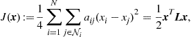 (7.22)
where ![]() denotes the network state vector.
denotes the network state vector.
2.07.3.1 Consensus algorithm
Given a set of measurements ![]() , for
, for ![]() , collected by the network nodes, the goal of consensus algorithm is to minimize the disagreement among the nodes. This can be useful, for example, when the nodes are measuring some common variable and their measurement is affected by error. The scope of the interaction among the nodes is to reduce the effect of errors on the final estimate. In fact, consensus is one of fundamental tools to design distributed decision algorithms that satisfy a global optimality principle, as corroborated by many works on distributed optimization, see, e.g., [14–20]. We recall now the consensus algorithm as this will form the basis of the distributed estimation and detection algorithms developed in the ensuing sections. Let us consider, for simplicity, the case where the nodes are measuring a temperature and the goal is to find the average temperature. In this case, reaching a consensus over the average temperature can be seen as the minimization of the disagreement, as defined in (7.22), between the states
, collected by the network nodes, the goal of consensus algorithm is to minimize the disagreement among the nodes. This can be useful, for example, when the nodes are measuring some common variable and their measurement is affected by error. The scope of the interaction among the nodes is to reduce the effect of errors on the final estimate. In fact, consensus is one of fundamental tools to design distributed decision algorithms that satisfy a global optimality principle, as corroborated by many works on distributed optimization, see, e.g., [14–20]. We recall now the consensus algorithm as this will form the basis of the distributed estimation and detection algorithms developed in the ensuing sections. Let us consider, for simplicity, the case where the nodes are measuring a temperature and the goal is to find the average temperature. In this case, reaching a consensus over the average temperature can be seen as the minimization of the disagreement, as defined in (7.22), between the states ![]() associated to the nodes.
associated to the nodes.
The minimization of the disagreement can be obtained by using a simple gradient-descent algorithm. More specifically, using a continuous-time system, the minimum of (7.22) can be achieved by running the following dynamical system [15]
![]() (7.23)
(7.23)
initialized with ![]() , where
, where ![]() is the vector containing all the initial measurements collected by the network nodes. This means that the state of each node evolves in time according to the first order differential equation
is the vector containing all the initial measurements collected by the network nodes. This means that the state of each node evolves in time according to the first order differential equation
![]() (7.24)
(7.24)
where ![]() indicates the set of neighbors of node i. Hence, every node updates its own state only by interacting with its neighbors.
indicates the set of neighbors of node i. Hence, every node updates its own state only by interacting with its neighbors.
Equation (7.23) assumes the form of a diffusion equation. Let us consider for example the evolution of a diffusing physical quantity ![]() as a function of the spatial variable z and of time t (
as a function of the spatial variable z and of time t (![]() could represent, for instance, the heat distribution), the diffusion equation assumes the form
could represent, for instance, the heat distribution), the diffusion equation assumes the form
![]() (7.25)
(7.25)
where D is the diffusion coefficient. If we discretize the space variable and approximate the second order derivative with a discrete-time second order difference, the diffusion Eq. (7.25) can be written as in (7.23), where the Laplacian matrix represents the discrete version of the Laplacian operator. This conceptual link between consensus equation and diffusion equation has been exploited in [21] to derive a fast consensus algorithm, mimicking the effect of advection. The interesting result derived in [21] is that to speed up the consensus (diffusion) process, it is necessary to use a directed graph, with time-varying adjacency matrix coefficients ![]() .
.
The solution of (7.23) is given by
![]() (7.26)
(7.26)
In the case analyzed so far, since the consensus algorithm has been deduced from the minimization of the disagreement and the disagreement has been defined for undirected graphs, the matrix ![]() is symmetric. Hence, its eigenvalues are real. The convergence of (7.26) is guaranteed because all the eigenvalues of
is symmetric. Hence, its eigenvalues are real. The convergence of (7.26) is guaranteed because all the eigenvalues of ![]() are non-negative, by construction. If the graph is connected, according to property P.2, the eigenvalue zero has multiplicity one. Furthermore, the eigenvector associated to the zero eigenvalue is the vector
are non-negative, by construction. If the graph is connected, according to property P.2, the eigenvalue zero has multiplicity one. Furthermore, the eigenvector associated to the zero eigenvalue is the vector ![]() . Hence, the system (7.23) converges to the consensus state:
. Hence, the system (7.23) converges to the consensus state:
![]() (7.27)
(7.27)
This means that every node converges to the average value of the measurements collected by the whole network, i.e.,
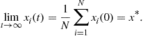 (7.28)
The convergence rate of system (7.24) is lower bounded by the slowest decaying mode of the dynamical system (7.23), i.e., by the second smallest eigenvalue of ![]() , also known as the algebraic connectivity of the graph [22]. More specifically, if the graph is connected or, equivalently, if
, also known as the algebraic connectivity of the graph [22]. More specifically, if the graph is connected or, equivalently, if ![]() , then the dynamical system (7.23) converges to consensus exponentially [15], i.e.,
, then the dynamical system (7.23) converges to consensus exponentially [15], i.e., ![]() with
with ![]() .
.
In some applications, the nodes are required to converge to a weighted consensus, rather than average consensus. This can be achieved with a slight modification of the consensus algorithm. If we premultiply the left side of (7.24) by a positive coefficient ![]() , the resulting equation
, the resulting equation
![]() (7.29)
(7.29)
converges to the weighted average
 (7.30)
This property will be used in deriving distributed estimation mechanisms in the next section.
Alternatively, the minimization of (7.22) can be achieved in discrete-time through the following iterative algorithm
![]() (7.31)
(7.31)
where we have introduced the so called transition matrix ![]() . Also in this case, the discrete time equation is initialized with the measurements taken by the sensor nodes at time 0, i.e.,
. Also in this case, the discrete time equation is initialized with the measurements taken by the sensor nodes at time 0, i.e., ![]() . This time, to guarantee convergence of the system (7.31), we need to choose the coefficient
. This time, to guarantee convergence of the system (7.31), we need to choose the coefficient ![]() properly. More specifically, the discrete time Eq. (7.31) converges if the eigenvalues of
properly. More specifically, the discrete time Eq. (7.31) converges if the eigenvalues of ![]() are bounded between
are bounded between ![]() and 1. This can be seen very easily considering that reiterating (7.31)k times, we get
and 1. This can be seen very easily considering that reiterating (7.31)k times, we get
![]() (7.32)
(7.32)
Let us denote by ![]() the eigenvectors of
the eigenvectors of ![]() associated to the eigenvalues
associated to the eigenvalues ![]() , with
, with ![]() . The eigenvalues of
. The eigenvalues of ![]() are real and we consider them ordered in increasing sense, so that
are real and we consider them ordered in increasing sense, so that ![]() . Hence, the evolution of system (7.32) can be written as
. Hence, the evolution of system (7.32) can be written as
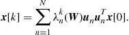 (7.33)
The matrix ![]() has an eigenvector equal to
has an eigenvector equal to ![]() , associated to the eigenvalue 1 by construction. In fact,
, associated to the eigenvalue 1 by construction. In fact, ![]() . If the graph is connected, the eigenvalue 1 of
. If the graph is connected, the eigenvalue 1 of ![]() has multiplicity one. Furthermore, if
has multiplicity one. Furthermore, if ![]() is chosen such that
is chosen such that ![]() , all other eigenvalues are less than 1. Hence, for a connected graph, the system (7.33) converges to
, all other eigenvalues are less than 1. Hence, for a connected graph, the system (7.33) converges to
![]() (7.34)
(7.34)
Again, this corresponds to having every node converging to the average consensus.
The consensus algorithm can be extended to the case of directed graphs. This case is indeed much richer of possibilities than the undirected case, because the consensus value ends up to depend more strictly on the graph topology. In the directed case, in fact, ![]() is an asymmetric matrix. The most important difference is that the graph connectivity turns out to depend on the orientation of the edges. Furthermore, each eigenvalue of
is an asymmetric matrix. The most important difference is that the graph connectivity turns out to depend on the orientation of the edges. Furthermore, each eigenvalue of ![]() gives rise to a pair of left and right eigenvectors which do not coincide with each other. These differences affect the final consensus state and induce different forms of consensus, as shown below.
gives rise to a pair of left and right eigenvectors which do not coincide with each other. These differences affect the final consensus state and induce different forms of consensus, as shown below.
The convergence of the system in (7.31) can be proved by exploiting the properties of non-negative matrices. A nonnegative matrix is row (or column) stochastic if all its row (or column) sums are equal to one. Furthermore if the graph associated to the network is strongly connected, i.e., the zero eigenvalue associated to ![]() has multiplicity one (see Appendix 2.07.9),
has multiplicity one (see Appendix 2.07.9), ![]() is called an irreducible matrix. An irreducible stochastic matrix is primitive if it has only one eigenvalue with maximum modulus. Primitive nonnegative matrices, often named Perron matrices, satisfy the Perron-Frobenius theorem [23].
is called an irreducible matrix. An irreducible stochastic matrix is primitive if it has only one eigenvalue with maximum modulus. Primitive nonnegative matrices, often named Perron matrices, satisfy the Perron-Frobenius theorem [23].
Theorem 1
Let![]() and
and![]() , respectively, the left and right eigenvectors associated to the unit eigenvalue of the primitive nonnegative matrix
, respectively, the left and right eigenvectors associated to the unit eigenvalue of the primitive nonnegative matrix![]() , i.e.,
, i.e.,![]() and
and![]() with
with![]() , then
, then![]() .
.
Let us now apply to a sensor network modeled by the graph ![]() , with adjacency matrix
, with adjacency matrix ![]() , the distributed consensus algorithm
, the distributed consensus algorithm
![]() (7.35)
(7.35)
with ![]() .
.
Interestingly, different forms of consensus can be achieved in a directed graph, depending on the graph connectivity properties [17]:
a. If the graph is strongly connected, the dynamical system in(7.35)converges to a weighted consensus, for any initial state vector ![]() , i.e.,
, i.e.,
![]() (7.36)
(7.36)
where ![]() ,
, ![]() , and
, and ![]() . In this case, since the graph is strongly connected,
. In this case, since the graph is strongly connected, ![]() is an irreducible matrix. Then, applying Gershgorin theorem [23], it can be deduced that there exists a single eigenvalue
is an irreducible matrix. Then, applying Gershgorin theorem [23], it can be deduced that there exists a single eigenvalue ![]() with maximum modulus. Then
with maximum modulus. Then ![]() is a primitive nonnegative matrix and from Theorem 1 the convergence in (7.36) is straightforward. In this case, every node contributes to the final consensus value. Furthermore, the consensus value is a weighted combination of the initial observations, where the weights are the entries of the left eigenvector associated to the null eigenvalue of
is a primitive nonnegative matrix and from Theorem 1 the convergence in (7.36) is straightforward. In this case, every node contributes to the final consensus value. Furthermore, the consensus value is a weighted combination of the initial observations, where the weights are the entries of the left eigenvector associated to the null eigenvalue of ![]() (or the unit eigenvalue of
(or the unit eigenvalue of ![]() ).
).
b. If the digraph is strongly connected and balanced, i.e.,![]() and
and![]() , the systems achieves an average consensus or
, the systems achieves an average consensus or![]() . In fact, for balanced graphs,
. In fact, for balanced graphs, ![]() is a double stochastic matrix with
is a double stochastic matrix with ![]() ;
;
c. If the digraph![]() is weakly connected (WC), but not strongly connected, and it contains a forest with K strongly connected root components, the graph splits in K disjoint clusters
is weakly connected (WC), but not strongly connected, and it contains a forest with K strongly connected root components, the graph splits in K disjoint clusters ![]() ,5 and all the nodes pertaining to each cluster converge to the consensus values
,5 and all the nodes pertaining to each cluster converge to the consensus values
![]() (7.37)
(7.37)
In words, there is no single consensus, in this case, but there is a local consensus within each cluster. Different clusters typically converge to different consensus values.
d. If the digraph![]() is composed of a single spanning tree, every node converges to the value assumed by the root node.
is composed of a single spanning tree, every node converges to the value assumed by the root node.
As far as the convergence rate, instead, in [15] it has been shown for undirected connected graphs that the dynamical system in (7.31) converges exponentially to the average consensus with a rate at least equal to ![]() where
where ![]() is the second largest eigenvalue of the Perron matrix
is the second largest eigenvalue of the Perron matrix ![]() . In fact by defining the disagreement vector
. In fact by defining the disagreement vector ![]() , it can be easily verified [15] that
, it can be easily verified [15] that ![]() evolves according to the disagreement dynamic given by
evolves according to the disagreement dynamic given by ![]() . Hence
. Hence ![]() represents a candidate Lyapunov function for the disagreement dynamics so that
represents a candidate Lyapunov function for the disagreement dynamics so that
![]() (7.38)
(7.38)
with ![]() since
since ![]() is a symmetric and primitive matrix. As a consequence the algorithm converges exponentially to consensus with a rate at least equal to
is a symmetric and primitive matrix. As a consequence the algorithm converges exponentially to consensus with a rate at least equal to![]() .
.
2.07.3.2 Consensus algorithms over realistic channels
So far, we have recalled the basic properties of consensus algorithm assuming that the exchange of information across the nodes occurs with no errors. In this section we study what happens to consensus algorithms when the communications among the nodes are affected by quantization errors, noise, packet drops, etc. The problem of consensus protocols affected by stochastic disturbance has been considered in a series of previous papers [24–29]. In [24], the authors use a decreasing sequence of weights to prove the convergence of consensus protocols to an agreement space in the presence of additive noise under a fixed network topology. The works in [25,26] consider consensus algorithms in the presence of link failures, which are modeled as i.i.d. Laplacian matrices of a directed graph. The papers present necessary and sufficient conditions for consensus exploiting the ergodicity of products of stochastic matrices. A distributed consensus algorithm in which the nodes utilize probabilistically quantized information to communicate with each other was proposed in [27]. As a result, the expected value of the consensus is equal to the average of the original sensor data. A stochastic approximation approach was followed in [28], which considered a stochastic consensus problem in a strongly connected directed graph where each agent has noisy measurements of its neighboring states. Finally, the study of a consensus protocol that is affected by both additive channel noise and a random topology was considered in [29]. The resulting algorithm relates to controlled Markov processes and the convergence analysis relies on stochastic approximation techniques.
In the study of consensus mechanisms over realistic channels, we consider the following sources of randomness:
1. Node positions: The first randomness is related to the spatial positions of the nodes, which are in general unknown. We model the spatial distribution of nodes as a random geometric graph composed of N nodes. In graph theory, a random geometric graph (RGG) is a random undirected graph drawn on a bounded region, eg. the unit disk, generated by:
a. Placing vertices at random uniformly and independently on the region,
b. Connecting two vertices, ![]() if and only if the distance between them is inside a threshold radius
if and only if the distance between them is inside a threshold radius ![]() , i.e.,
, i.e., ![]() .
.
Several probabilistic results are known about RGG’s. In particular, as shown in [3], if N nodes are placed in a disc of unit area in ![]() and each node transmits with a power scaling with N as in (7.2), the resulting network is asymptotically connected with probability one, as
and each node transmits with a power scaling with N as in (7.2), the resulting network is asymptotically connected with probability one, as ![]() .
.
2. Random link failures model: In a realistic communication scenario, the packets exchanged among sensors may be received with errors, because of channel fading or noise. The retransmission of erroneous packets can be incorporated into the system, but packet retransmission introduces a nontrivial additional complexity in decentralized implementations and, most important, it introduces an unknown delay and delay jitter. It is then of interest to examine simple protocols where erroneous packets are simply dropped. Random packet dropping can be taken into account by modeling the coefficient ![]() describing the network topology as random variables that assume the value 1 or 0, if the packet is correctly delivered or not, respectively. In this case, the Laplacian varies with time as a sequence of i.i.d. matrices
describing the network topology as random variables that assume the value 1 or 0, if the packet is correctly delivered or not, respectively. In this case, the Laplacian varies with time as a sequence of i.i.d. matrices ![]() , which can be written, without any loss of generality, as
, which can be written, without any loss of generality, as
![]() (7.39)
(7.39)
where ![]() denotes the mean matrix and
denotes the mean matrix and ![]() are i.i.d. perturbations around the mean. We do not make any assumptions about the link failure model. Although the link failures and the Laplacians are independent over time, during the same iteration, the link failures can still be spatially correlated. It is important to remark that we do not require the random instantiations
are i.i.d. perturbations around the mean. We do not make any assumptions about the link failure model. Although the link failures and the Laplacians are independent over time, during the same iteration, the link failures can still be spatially correlated. It is important to remark that we do not require the random instantiations ![]() of the graph be connected for all k. We only require the graph to be connected on average. This condition is captured by requiring
of the graph be connected for all k. We only require the graph to be connected on average. This condition is captured by requiring ![]() .
.
3. Dithered quantization: We assume that each node encodes the message to be exchanged with the other nodes using a uniform quantizer, with a finite number of bits ![]() , defined by the following vector mapping,
, defined by the following vector mapping, ![]() ,
,
![]() (7.40)
(7.40)
where the entries of the vector ![]() , the quantization step
, the quantization step ![]() , and the error
, and the error ![]() satisfy
satisfy
![]() (7.41)
(7.41)
![]() (7.42)
(7.42)
The quantization alphabet is
![]() (7.43)
(7.43)
Conditioned on the input, the quantization error ![]() is deterministic. This induces a correlation among the quantization errors resulting at different nodes and different times, which may affect the convergence properties of the distributed algorithm. To avoid undesired error correlations, we introduce dithering, as in [30,31]. In particular, the dither added to randomize the quantization effects satisfies a special condition, namely the Schuchman conditions, as in subtractively dithered systems, [32]. Then, at every time instant k, adding to each component
is deterministic. This induces a correlation among the quantization errors resulting at different nodes and different times, which may affect the convergence properties of the distributed algorithm. To avoid undesired error correlations, we introduce dithering, as in [30,31]. In particular, the dither added to randomize the quantization effects satisfies a special condition, namely the Schuchman conditions, as in subtractively dithered systems, [32]. Then, at every time instant k, adding to each component ![]() a dither sequence
a dither sequence ![]() of i.i.d. uniformly distributed random variables on
of i.i.d. uniformly distributed random variables on ![]() independent of the input sequence, the resultant error sequence
independent of the input sequence, the resultant error sequence ![]() becomes
becomes
![]() (7.44)
(7.44)
The sequence ![]() is now an i.i.d. sequence of uniformly distributed random variables on
is now an i.i.d. sequence of uniformly distributed random variables on ![]() , which is independent of the input sequence.
, which is independent of the input sequence.
The convergence of consensus algorithm in the presence of random disturbance can be proved by exploiting results from supermartingale theory [33]. In an ideal communication case, by selecting the step-size of the algorithm to be sufficiently small (smaller than ![]() , where
, where ![]() is the maximum eigenvalue of the Laplacian matrix of the graph), the discrete-time consensus algorithm will asymptotically converge to the agreement subspace. However, in a realistic communication scenario, the links among the sensors may fail randomly and the exchanged data is corrupted by quantization noise. Under these nonideal conditions, the consensus algorithm needs to be properly adjusted to guarantee convergence. A discrete time consensus algorithm that accounts for random link failures and dithered quantization noise can be written as:
is the maximum eigenvalue of the Laplacian matrix of the graph), the discrete-time consensus algorithm will asymptotically converge to the agreement subspace. However, in a realistic communication scenario, the links among the sensors may fail randomly and the exchanged data is corrupted by quantization noise. Under these nonideal conditions, the consensus algorithm needs to be properly adjusted to guarantee convergence. A discrete time consensus algorithm that accounts for random link failures and dithered quantization noise can be written as:
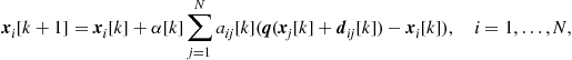 (7.45)
where ![]() is a positive iteration dependent step-size, and
is a positive iteration dependent step-size, and ![]() is the dithered quantization vector. Now, exploiting the feature of subtractively dithered systems in (7.44), the previous expression can be recast as:
is the dithered quantization vector. Now, exploiting the feature of subtractively dithered systems in (7.44), the previous expression can be recast as:
 (7.46)
Starting from some initial value, ![]() , each node generates via (7.46) a sequence of state variables,
, each node generates via (7.46) a sequence of state variables, ![]() . The value
. The value ![]() at the ith node at time
at the ith node at time ![]() is a function of: its previous state
is a function of: its previous state ![]() and the quantized states correctly received at time k by the neighboring sensors. As described previously, the data are subtractively dithered-quantized, so that the quantized data received by the ith sensor from the jth sensor at time k is
and the quantized states correctly received at time k by the neighboring sensors. As described previously, the data are subtractively dithered-quantized, so that the quantized data received by the ith sensor from the jth sensor at time k is ![]() . It then follows that the quantization error
. It then follows that the quantization error ![]() is a random vector, whose components are i.i.d., uniformly distributed on
is a random vector, whose components are i.i.d., uniformly distributed on ![]() , and independent of
, and independent of ![]() .
.
One way to guarantee convergence of the previous system is to use a positive iteration-dependent step size ![]() satisfying [24,29]
satisfying [24,29]
![]() (7.47)
(7.47)
Exploiting results from stochastic approximation theory, this choice drives the noise variance to zero while guaranteeing the convergence to the consensus subspace.
A numerical example is useful to show the robustness of consensus algorithm in the presence of link failures and quantization noise. We consider a connected network composed of 20 nodes as depicted on the left side of Figure 7.5. The initial value of the state variable at each node is randomly chosen in the interval ![]() . At the kth iteration of the updating rule (7.45), each node communicates to its neighbors its current state, i.e., a scalar
. At the kth iteration of the updating rule (7.45), each node communicates to its neighbors its current state, i.e., a scalar ![]() . Because of fading and additive noise, a communication link among two neighbors has a certain probability p to be established correctly. The values to be exchanged are (dither) quantized with 6 bits. The iteration-dependent step size is chosen as
. Because of fading and additive noise, a communication link among two neighbors has a certain probability p to be established correctly. The values to be exchanged are (dither) quantized with 6 bits. The iteration-dependent step size is chosen as ![]() , with
, with ![]() , in order to satisfy (7.47). The right side of Figure 7.5 shows the average behavior of the disagreement among the sensors in the network, versus the iteration index, for different values of the probability p to establish a communication link correctly. The result is averaged over 100 independent realizations. The ideal case corresponds to
, in order to satisfy (7.47). The right side of Figure 7.5 shows the average behavior of the disagreement among the sensors in the network, versus the iteration index, for different values of the probability p to establish a communication link correctly. The result is averaged over 100 independent realizations. The ideal case corresponds to ![]() and it is shown as a benchmark. As we can notice from the right side of Figure 7.5, even in the presence of random disturbances, an agreement is always reached by the network for any value of p. The only effect of the random link failures is to slow down the convergence process, without altering the final value of the global potential function. This proves the robustness of the algorithm.
and it is shown as a benchmark. As we can notice from the right side of Figure 7.5, even in the presence of random disturbances, an agreement is always reached by the network for any value of p. The only effect of the random link failures is to slow down the convergence process, without altering the final value of the global potential function. This proves the robustness of the algorithm.

2.07.4 Distributed estimation
Having introduced all the tools necessary to study distributed estimation and detection mechanisms, let us now start with the estimation problem. This problem has been the subject of an extensive literature, see, e.g., [34–43]. Most of the algorithms proposed in these works propose a mix of local estimation and consensus among neighbor nodes to improve upon the performance of the local estimators. In a first class of methods, like [35,36] for example, the nodes collect all the data first, perform local estimation and then interact iteratively with their neighbors. In alternative methods, the nodes keep interacting with each other while collecting new measurements or, in general, receiving new information, like in [37,38,42]. These two classes of methods can be seen as assigning different time scales to the local estimation and consensus steps. Indeed, it can be proved that a proper combination of local estimation and consensus can bring the whole network to a globally optimal estimate, provided that the graph describing the interaction among the nodes is connected. This approach was pursued, for example in [35], where the so called bridge nodes fulfilled the scope of enforcing local consensus. In the following, we will show how alternative formulations of the globally optimal estimation problem naturally lead to a different mix of the local estimation and the consensus steps, without the need to introduce any node having a special role nor enforcing different time scales a priori.
Let us denote with ![]() the parameter vector to be estimated. In some cases, there is no prior information about
the parameter vector to be estimated. In some cases, there is no prior information about ![]() . In other cases,
. In other cases, ![]() is known to belong to a given set
is known to belong to a given set ![]() : For instance, its entries are known to be positive or to belong to a finite interval of known limits, and so on. In some applications,
: For instance, its entries are known to be positive or to belong to a finite interval of known limits, and so on. In some applications, ![]() may be the outcome of a random variable described by a known pdf
may be the outcome of a random variable described by a known pdf ![]() . Let us denote by
. Let us denote by ![]() the measurement vector collected by node i and by
the measurement vector collected by node i and by ![]() the whole set of data collected by all the nodes. In the two cases of interest, the estimation can be obtained as the solution of the following problems:Arbitrary case
the whole set of data collected by all the nodes. In the two cases of interest, the estimation can be obtained as the solution of the following problems:Arbitrary case
![]() (7.48)
(7.48)
![]() (7.49)
(7.49)
where ![]() is the joint pdf of vector
is the joint pdf of vector ![]() , for a given arbitrary vector
, for a given arbitrary vector ![]() , orRandom case
, orRandom case
![]() (7.50)
(7.50)
where ![]() is (known) prior pdf of the parameter vector and
is (known) prior pdf of the parameter vector and ![]() is the pdf of
is the pdf of ![]() conditioned to
conditioned to ![]() .
.
In general, it is not necessary to reconstruct the whole joint pdf ![]() (or
(or ![]() ) to obtain the optimal estimate. Let us consider, for example, the case where the pdf can be factorized as
) to obtain the optimal estimate. Let us consider, for example, the case where the pdf can be factorized as
![]() (7.51)
(7.51)
where ![]() depends on
depends on ![]() only through
only through ![]() , whereas
, whereas ![]() does not depend on
does not depend on ![]() . The function
. The function ![]() is called a sufficient statistic for
is called a sufficient statistic for ![]() [44]. In general, the sufficient statistic
[44]. In general, the sufficient statistic ![]() is a vector, as it may be constituted by a set of functions.
is a vector, as it may be constituted by a set of functions.
If (7.51) holds true, all is necessary to estimate ![]() is not really
is not really ![]() , but only
, but only ![]() . This means that any sensor able to evaluate
. This means that any sensor able to evaluate ![]() through an interaction with the other sensors is able to find out the optimal parameter vector
through an interaction with the other sensors is able to find out the optimal parameter vector ![]() as the vector that maximizes
as the vector that maximizes ![]() .
.
A simple (yet common) example is given by the so called exponential family of pdf
![]() (7.52)
(7.52)
Examples of random variables described by this class include the Gaussian, Rayleigh, and exponential pdf’s. Hence, this is a rather common model. Let us assume now that the observations ![]() collected by different nodes are statistically independent and identically distributed (i.i.d.), according to (7.52). It is easy to check, simply applying the definition in (7.51), that a sufficient statistic in such a case is the scalar function:
collected by different nodes are statistically independent and identically distributed (i.i.d.), according to (7.52). It is easy to check, simply applying the definition in (7.51), that a sufficient statistic in such a case is the scalar function:
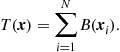 (7.53)
This structure suggests that a simple distributed way to enable every node in the network to estimate the vector ![]() locally, without loss of optimality with respect to the centralized approach, is to run a consensus algorithm, where the initial state of every node is set equal to
locally, without loss of optimality with respect to the centralized approach, is to run a consensus algorithm, where the initial state of every node is set equal to ![]() . At convergence, if the network is connected, every node has a state equal to the consensus value, i.e.,
. At convergence, if the network is connected, every node has a state equal to the consensus value, i.e., ![]() . This enables every node to implement the optimal estimation by simply interacting with its neighbors to achieve a consensus. The only necessary condition for this simple method to work properly is that the network be connected. This is indeed a very simple example illustrating how consensus can be a fundamental step in deriving an optimal estimation through a purely decentralized approach relying only upon the exchange of data among neighbors.
. This enables every node to implement the optimal estimation by simply interacting with its neighbors to achieve a consensus. The only necessary condition for this simple method to work properly is that the network be connected. This is indeed a very simple example illustrating how consensus can be a fundamental step in deriving an optimal estimation through a purely decentralized approach relying only upon the exchange of data among neighbors.
In the next two sections, we will analyze in more details the purely distributed case (with no fusion center) where the global estimation can be carried out in any node and the centralized case, where the final estimation is taken at the fusion center.
2.07.4.1 Decentralized observations with decentralized estimation
In the following we analyze different observation models and illustrate alternative distributed estimation algorithms. We will start with the conditionally independent case and then we will generalize the approach to a conditionally dependent model.
2.07.4.1.1 Conditionally independent observations
A case amenable for finding distributed solutions is given by the situations where the observations collected by different sensors are conditionally independent. In such a case, the joint pdf ![]() can be factorized as follows
can be factorized as follows
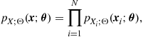 (7.54)
where ![]() is the pdf of the vector
is the pdf of the vector ![]() observed by node i. Taking the
observed by node i. Taking the ![]() of this expression, the optimization problem can be cast, equivalently, as
of this expression, the optimization problem can be cast, equivalently, as
 (7.55)
Even if the objective function to be maximized is written as a sum of functions depending each on a local observation vector, the solution of the previous problem still requires a centralized approach because the vector ![]() to be estimated is common to all the terms. A possible way to find a distributed solution to the problem in (7.55) consists in introducing an instrumental common variable
to be estimated is common to all the terms. A possible way to find a distributed solution to the problem in (7.55) consists in introducing an instrumental common variable ![]() and rewriting the previous problem in the following form
and rewriting the previous problem in the following form
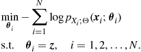 (7.56)
This is a constrained problem, whose Lagrangian is
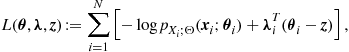 (7.57)
where ![]() are the vectors whose entries are the Lagrange multipliers associated to the equality constraints in (7.56). In many cases, it is useful to introduce the so called augmented Lagrangian [45]:
are the vectors whose entries are the Lagrange multipliers associated to the equality constraints in (7.56). In many cases, it is useful to introduce the so called augmented Lagrangian [45]:
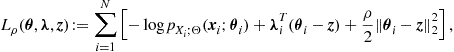 (7.58)
where ![]() is a penalty parameter. Minimizing the augmented Lagrangian leads to the same solution as minimizing the original Lagrangian because any feasible vector satisfying the linear constraint yields a zero penalty. Nevertheless, there are some benefits in working with the augmented Lagrangian, namely: i) the objective function is differentiable under milder conditions than with the original Lagrangian; ii) convergence can be achieved without requiring strict convexity of the objective function (see [45] for more insight into the augmented Lagrangian method).
is a penalty parameter. Minimizing the augmented Lagrangian leads to the same solution as minimizing the original Lagrangian because any feasible vector satisfying the linear constraint yields a zero penalty. Nevertheless, there are some benefits in working with the augmented Lagrangian, namely: i) the objective function is differentiable under milder conditions than with the original Lagrangian; ii) convergence can be achieved without requiring strict convexity of the objective function (see [45] for more insight into the augmented Lagrangian method).
If the pdf’s involved in (7.58) are log-concave functions of ![]() , the problem in (7.58) is strongly convex and then it admits a unique solution and there are efficient algorithms to compute the solution. Here, we are interested in deriving decentralized solutions.
, the problem in (7.58) is strongly convex and then it admits a unique solution and there are efficient algorithms to compute the solution. Here, we are interested in deriving decentralized solutions.
A possible method to find a distributed solution of the problem in (7.58) is the alternating direction method of multipliers (ADMM)[45]. An excellent recent review of ADMM and its applications is [46]. The application of ADMM to distributed estimation problems was proposed in [35]. The method used in [35] relied on the introduction of the so called bridge nodes. Here, we will describe methods that do not require the introduction of any special class of nodes (in principle, every node has the same functionality as any other node). This is useful to simplify the estimation method as well as network design and management.
The ADMM algorithm applied to solve (7.58) works through the following steps:
 (7.59)
The first and second steps aim at minimizing the primal function (i.e., the augmented Lagrangian) over the unknown variables ![]() and
and ![]() , for a given value of the Lagrange multipliers’ vectors
, for a given value of the Lagrange multipliers’ vectors ![]() , as computed in the previous iteration.
, as computed in the previous iteration.
The third step is a dual variable update, whose goal is to maximize the dual function, as in the dual ascent method. We recall that, in our case, the dual function is defined as
![]() (7.60)
(7.60)
In ADMM, the dual ascent step uses a gradient ascent approach to update ![]() in order to maximize
in order to maximize ![]() , for a given value of vectors
, for a given value of vectors ![]() and
and ![]() , with the important difference that the step size used to compute the update is exactly the penalty coefficient
, with the important difference that the step size used to compute the update is exactly the penalty coefficient ![]() .
.
In our case, the second step can be computed in closed form as follows
![]() (7.61)
(7.61)
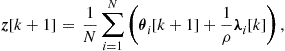 (7.62)
![]() (7.63)
(7.63)
From this formulation, we can see that the first and third steps can be run in parallel, over each node. The only step that requires an exchange of values among the nodes is the second step that requires the computation of an average value. But, as we know from previous section, the average value can be computed through a distributed consensus algorithm. The only condition for the convergence of consensus algorithm to the average value is that the graph representing the links among the nodes is connected.
The step in (7.62) can be further simplified as follows. Let us denote with ![]() the averaging operation across the nodes, i.e.,
the averaging operation across the nodes, i.e.,
 (7.64)
Using this notation, the ![]() -update can be written as
-update can be written as
![]() (7.65)
(7.65)
Similarly, averaging over the ![]() -update yields
-update yields
![]() (7.66)
(7.66)
Substituting (7.65) in (7.66), it is easy to check that, after the first iteration, ![]() . Hence, using
. Hence, using ![]() , the overall algorithm proceeds as indicated in Table 7.1.
, the overall algorithm proceeds as indicated in Table 7.1.
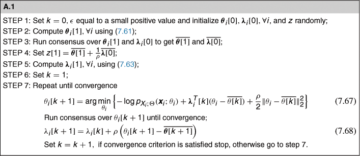
The convergence criterion used in the steps of the algorithm is based on the relative absolute difference at two successive iterations: Given a sequence ![]() , the algorithm stops when
, the algorithm stops when ![]() , with
, with ![]() a small positive value.
a small positive value.
Equations (7.67)–(7.68) give rise to an interesting interpretation: the primal update (first equation) aims at implementing a local optimization, with a penalty related to the disagreement between the local solution and the global one; the dual update (second equation) aims at driving all the local solutions to converge to a common (consensus) value, which coincides with the globally optimal solution.
The straightforward implementation of (16.1) and (16.1) requires running, at each step k of the ADMM algorithm, a consensus algorithm. A possible alternative approach can be envisaged by reformulating the optimization problem as follows:
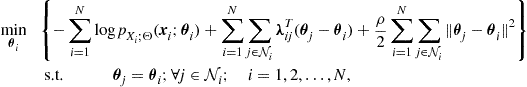 (7.69)
where ![]() denotes the set of node i’s neighbors. To make more clear the interaction among the nodes, it is useful to introduce the graph notation, as in previous section. Using the adjacency matrix
denotes the set of node i’s neighbors. To make more clear the interaction among the nodes, it is useful to introduce the graph notation, as in previous section. Using the adjacency matrix ![]() , the previous problem can be rewritten as follows:
, the previous problem can be rewritten as follows:
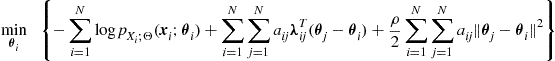 (7.70)
![]()
This formulation does not require the introduction of the instrumental variable ![]() . We keep enforcing the constraint that all the local estimates
. We keep enforcing the constraint that all the local estimates ![]() converge to the same value. However, the penalty is now formulated as the disagreement between the local estimates. From consensus algorithm, we know that nulling the disagreement is equivalent to forcing all the vectors
converge to the same value. However, the penalty is now formulated as the disagreement between the local estimates. From consensus algorithm, we know that nulling the disagreement is equivalent to forcing all the vectors ![]() to reach the same value if the graph describing the interactions among the nodes is connected. Hence, if the network is connected, at convergence, the disagreement goes to zero and there is no bias resulting from the introduction of the disagreement penalty.
to reach the same value if the graph describing the interactions among the nodes is connected. Hence, if the network is connected, at convergence, the disagreement goes to zero and there is no bias resulting from the introduction of the disagreement penalty.
The formulation in (7.70) is more amenable for an implementation that does not require, at any step of the algorithm, the convergence of consensus algorithms. In fact, applying ADMM to the solution of (7.70) yields the algorithm described in Table 7.2.
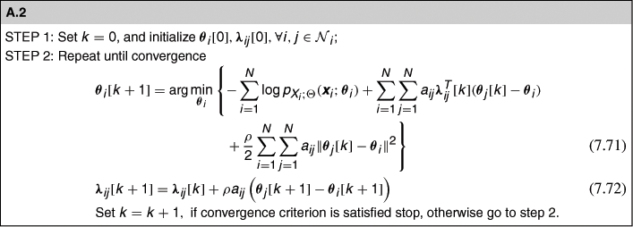
Some examples of applications are useful to grasp the main features of these algorithms.
2.07.4.1.2 Distributed ML estimation under Gaussian noise
Let us consider the common situation where the measured vector ![]() is related to the parameter vector
is related to the parameter vector ![]() , with
, with ![]() , through a linear observation model, as:
, through a linear observation model, as:
![]() (7.73)
(7.73)
where ![]() and
and ![]() is a vector of jointly Gaussian random variables with zero mean and covariance matrix
is a vector of jointly Gaussian random variables with zero mean and covariance matrix ![]() , i.e.,
, i.e., ![]() .
.
In such a case, algorithm A.1 in (7.67) simplifies as the first step of (7.67) can be expressed in closed form
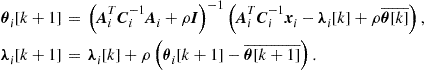 (7.74)
The two updates can be computed in parallel by all the nodes, after having computed the average values through the consensus algorithm.
Alternatively, algorithm A.2 becomes
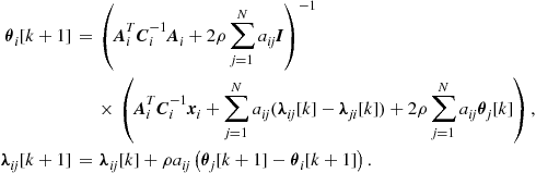 (7.75)
In this case, there is no need of running the consensus algorithm for every iteration. Some numerical results are useful to compare the methods. As an example, we considered a connected network composed of ![]() sensors. We set
sensors. We set ![]() and assumed an observation vector of size
and assumed an observation vector of size ![]() . In Figure 7.6 we report the estimates
. In Figure 7.6 we report the estimates ![]() , for
, for ![]() , versus the iteration index m, for the two algorithms A.1 (left plot) and A.2 (right plot). The iteration index m includes also the iterations necessary for the consensus algorithm to converge within a prescribed accuracy (in this case, we stopped the consensus algorithm as soon as the absolute difference between two consecutive updates is below of
, versus the iteration index m, for the two algorithms A.1 (left plot) and A.2 (right plot). The iteration index m includes also the iterations necessary for the consensus algorithm to converge within a prescribed accuracy (in this case, we stopped the consensus algorithm as soon as the absolute difference between two consecutive updates is below of ![]() for all the nodes). In both figures, we report, as a benchmark, the maximum likelihood estimate (horizontal x-marked line) achievable by a centralized node that knows all the observation vectors and all the model parameters, i.e.,
for all the nodes). In both figures, we report, as a benchmark, the maximum likelihood estimate (horizontal x-marked line) achievable by a centralized node that knows all the observation vectors and all the model parameters, i.e., ![]() . From Figure 7.6, we can see that the estimates obtained with both methods converge to the optimal ML estimates.
. From Figure 7.6, we can see that the estimates obtained with both methods converge to the optimal ML estimates.
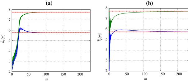
Figure 7.6 Per node parameter estimation versus the iteration index m using algorithms A.1 (left) and A.2 (right).
In the specific case where the observation model is as in (7.73), with additive Gaussian noise, and the noise vectors pertaining to different sensors are mutually uncorrelated, the globally optimal ML estimate is
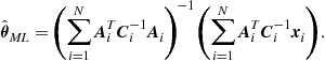 (7.76)
This formula is a vector weighted sum of the observations. Recalling that consensus algorithms, if properly initialized, can be made to converge to a weighted sum of the initial states, we can use the consensus algorithm directly to compute the globally optimal ML estimate through a totally distributed mechanism. In particular, in this case, the consensus algorithm proceeds as in Table 7.3.
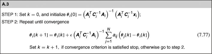
Using again the basic properties of consensus algorithm, if the graph is connected and the step size ![]() is sufficiently small, the iterations in (7.77) converge to the globally optimal estimate (7.76).
is sufficiently small, the iterations in (7.77) converge to the globally optimal estimate (7.76).
2.07.4.1.3 Distributed Bayesian estimation under Gaussian noise and Laplacian prior
Let us consider now the case where the parameter vector is a random vector with known prior probability density function. Following a Bayesian approach, as in (7.50), the practical difference is that in such a case the objective function must include a term depending on the prior probability. Let us consider, for instance, the interesting case where the observation is Gaussian, as in the previous example, and the prior pdf is Laplacian, i.e.,
![]() (7.78)
(7.78)
with ![]() , where
, where ![]() denotes the
denotes the ![]() norm of vector
norm of vector ![]() . In this case, the problem to be solved is the following
. In this case, the problem to be solved is the following
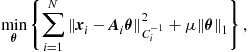 (7.79)
where ![]() denotes the weighted
denotes the weighted ![]() norm of
norm of ![]() , i.e.,
, i.e., ![]() .
.
Interestingly, this formulation coincides with the formulation resulting from having no prior pdf, but incorporating an ![]() norm in order to drive the solution towards a sparse vector. This is the so called least-absolute shrinkage and selection operator (lasso) method [47]. A distributed algorithm to solve a linear regression problem with sparsity constraint was proposed in [48]. Here we provide a similar approach, with the important difference that, in each iteration, the update is computed in closed form. A decentralized solution can be found by reformulating the problem as follows
norm in order to drive the solution towards a sparse vector. This is the so called least-absolute shrinkage and selection operator (lasso) method [47]. A distributed algorithm to solve a linear regression problem with sparsity constraint was proposed in [48]. Here we provide a similar approach, with the important difference that, in each iteration, the update is computed in closed form. A decentralized solution can be found by reformulating the problem as follows
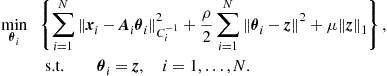 (7.80)
Using the ADMM approach, the algorithm proceeds through the following updates
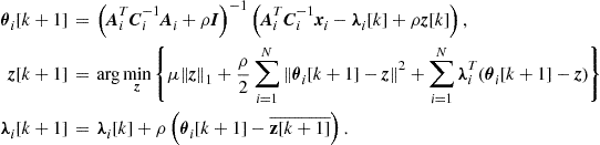 (7.81)
The second equation can also be expressed in closed form. Moreover, defining the vector threshold function ![]() as the vector whose entries are obtained by applying the scalar thresholding function
as the vector whose entries are obtained by applying the scalar thresholding function ![]() to each element of vector
to each element of vector ![]() , where
, where
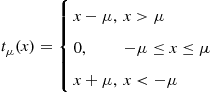 (7.82)
the overall algorithm is as in Table 7.4.

As a numerical example, in Figure 7.7 we report the behavior of the estimated variable obtained using Algorithm A.4 versus the iteration index m, which includes the convergence times of two consensus algorithms in the equation (7.84).

Figure 7.7 Per node estimated variable versus the iteration index m for distributed Bayesian estimation using the ADMM approach.
The example refers to a network of ![]() nodes, using
nodes, using ![]() . The horizontal x-marked line represents the centralized optimal solution. The parameter vector of this example has two components, one of which has been set to zero to test the capability to recover the sparsity. We can notice from Figure 7.7 that, as expected, the algorithm converges to the globally optimal values.
. The horizontal x-marked line represents the centralized optimal solution. The parameter vector of this example has two components, one of which has been set to zero to test the capability to recover the sparsity. We can notice from Figure 7.7 that, as expected, the algorithm converges to the globally optimal values.
To show the impact of the penalty coefficient ![]() on the sparsity of the estimated vector, in Figure 7.8 we have reported the average mean square estimation error versus the coefficient
on the sparsity of the estimated vector, in Figure 7.8 we have reported the average mean square estimation error versus the coefficient ![]() , defined as the fraction of zeros entries in the vector
, defined as the fraction of zeros entries in the vector ![]() to be estimated, for different values of
to be estimated, for different values of ![]() . It can be noted from Figure 7.8 that for
. It can be noted from Figure 7.8 that for ![]() the optimal solution is independent by
the optimal solution is independent by ![]() and it coincides with the optimal (centralized) ML solution. Furthermore, we can observe that, as
and it coincides with the optimal (centralized) ML solution. Furthermore, we can observe that, as ![]() and
and ![]() increase, the average estimation error decreases thanks to the recovering sparsity property of the ADMM approach with the lasso constraint.
increase, the average estimation error decreases thanks to the recovering sparsity property of the ADMM approach with the lasso constraint.

2.07.4.1.4 Distributed recursive least square estimation with sparsity constraint
In some applications, the parameters to be estimated may be changing over time. In these cases, it is more advisable to adopt recursive procedure rather than the batch approach followed until now. We show now how to obtain a distributed recursive least square (RLS) estimation incorporating a sparsity constraint.
Let us assume a linear observation model
![]() (7.86)
(7.86)
where ![]() denotes the observation taken by node i at time
denotes the observation taken by node i at time ![]() is a known, possibly time-varying, mixing matrix and
is a known, possibly time-varying, mixing matrix and ![]() is the observation noise, supposed to have zero mean and covariance matrix
is the observation noise, supposed to have zero mean and covariance matrix ![]() .
.
In RLS estimation with a sparsity constraint, the goal is to find the parameter vector ![]() , at each time instant n, that minimizes the following objective function
, at each time instant n, that minimizes the following objective function
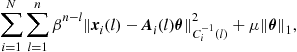 (7.87)
where ![]() is a forgetting factor used to weight more the most recent observations with respect to the older ones. The coefficient
is a forgetting factor used to weight more the most recent observations with respect to the older ones. The coefficient ![]() weights the importance of the sparsity constraint.
weights the importance of the sparsity constraint.
Proceeding as in the previous examples, a distributed solution can be found by formulating the problem, at each time n, as a constrained problem incorporating an instrumental variable ![]() to force all the nodes to converge to a common estimate. The problem can be made explicit as
to force all the nodes to converge to a common estimate. The problem can be made explicit as
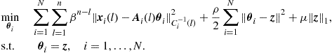 (7.88)
Again, the solution can be achieved by applying ADMM and the result is given by the algorithm described in Table 7.5
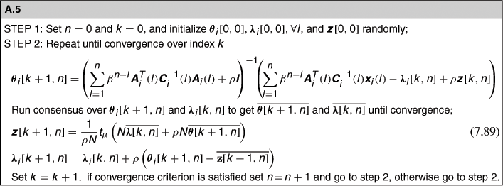
As before, the only step requiring the interaction among the nodes is a consensus algorithm to be run to compute the averages appearing in equation (7.89).
To test the convergence of Algorithm A.5, we considered a possible application to cooperative sensing for cognitive radio. We assumed the presence of a macro base station transmitting using a multicarrier scheme. We considered for simplicity of representation four channels, but the method can be easily extended to a larger number of channels. The sensing nodes aim to recover the activity of the macro transmitter, represented by a vector ![]() composed of four entries, one for each channel. To improve the accuracy of the local estimation, the sensors cooperate with each other by running Algorithm A.5. At some time, the activity level switches from on to off or viceversa. As an example, in Figure 7.9 we report the four parameters to be estimated, indicated by the unmarked lines. At time
composed of four entries, one for each channel. To improve the accuracy of the local estimation, the sensors cooperate with each other by running Algorithm A.5. At some time, the activity level switches from on to off or viceversa. As an example, in Figure 7.9 we report the four parameters to be estimated, indicated by the unmarked lines. At time ![]() , the parameters switch to test the tracking capability of the proposed method.
, the parameters switch to test the tracking capability of the proposed method.
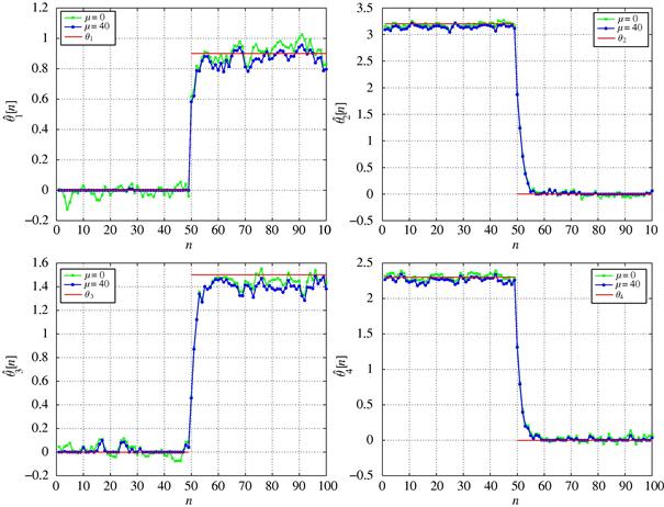
Figure 7.9 Estimated parameters versus the number of current observations n for the RLS algorithm, assuming ![]() ,
, ![]() , and
, and ![]() .
.
In Figure 7.9 we draw also the estimated parameters ![]() for
for ![]() versus the current observation index n. We used
versus the current observation index n. We used ![]() and two values of the sparsity coefficient:
and two values of the sparsity coefficient: ![]() and
and ![]() . We can notice from Figure 7.9 that the method is able to track the true parameters. It is also interesting to see that, as the penalty coefficient
. We can notice from Figure 7.9 that the method is able to track the true parameters. It is also interesting to see that, as the penalty coefficient ![]() increases, the zero coefficients are estimated with greater accuracy. Conversely, the positive coefficients are recovered with a slightly larger bias.
increases, the zero coefficients are estimated with greater accuracy. Conversely, the positive coefficients are recovered with a slightly larger bias.
To evaluate the impact of the forgetting factor ![]() on the accuracy and tracking capability of the distributed RLS method, in Figure 7.10 we reported the estimated parameters. using
on the accuracy and tracking capability of the distributed RLS method, in Figure 7.10 we reported the estimated parameters. using ![]() and
and ![]() , having set
, having set ![]() . It can be noted that, as
. It can be noted that, as ![]() increases, the larger memory of the filter yields more accurate estimates. At the same time, having a larger memory implies slower time to reaction to the parameter switch, as evidenced in Figure 7.10.
increases, the larger memory of the filter yields more accurate estimates. At the same time, having a larger memory implies slower time to reaction to the parameter switch, as evidenced in Figure 7.10.
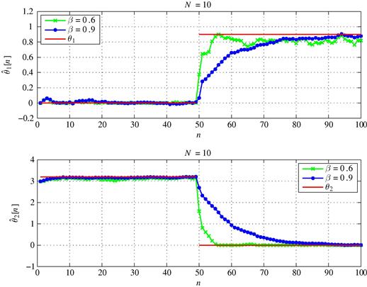
Figure 7.10 Parameter estimation versus the number of observations n of the recursive least square estimation using the ADMM approach, considering ![]() and two different values of
and two different values of ![]() .
.
For any given forgetting factor ![]() , the only possibility to improve the estimation accuracy is to have more nodes sensing a common macro base station. As an example, in Figure 7.11 we report the behavior of the estimates obtained with different number of nodes, for a forgetting factor
, the only possibility to improve the estimation accuracy is to have more nodes sensing a common macro base station. As an example, in Figure 7.11 we report the behavior of the estimates obtained with different number of nodes, for a forgetting factor ![]() . We can notice that, as expected, increasing the number of nodes, the estimation accuracy increases as well. This reveals a trade-off between forgetting factor (time memory) and number of nodes involved in cooperative sensing.
. We can notice that, as expected, increasing the number of nodes, the estimation accuracy increases as well. This reveals a trade-off between forgetting factor (time memory) and number of nodes involved in cooperative sensing.

2.07.4.1.5 Distributed parameter estimation in spatially correlated observations
So far, we have analyzed the case of conditionally independent observations. Let us consider now the case where the observation noise is spatially correlated. More specifically, we assume here the following observation model, for each sensor
![]() (7.90)
(7.90)
where the noise variables ![]() are jointly Gaussian with zero mean and covariance matrix
are jointly Gaussian with zero mean and covariance matrix ![]() , or precision matrix
, or precision matrix ![]() . Furthermore, we assume that
. Furthermore, we assume that ![]() is a Gaussian Markov random field, so that the precision matrix is typically a sparse matrix. The joint pdf of the observation vector can then be written as in (7.17), i.e.,
is a Gaussian Markov random field, so that the precision matrix is typically a sparse matrix. The joint pdf of the observation vector can then be written as in (7.17), i.e.,
 (7.91)
where ![]() can be rewritten as follows
can be rewritten as follows
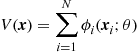 (7.92)
with ![]() , and
, and
![]() (7.93)
(7.93)
As in the previous cases, also here a decentralized solution can be reached by formulating the problem as the minimization of the augmented Lagrangian
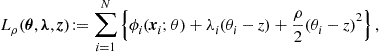 (7.94)
subject to ![]() . Applying the ADMM algorithm to this case, we get the following algorithm
. Applying the ADMM algorithm to this case, we get the following algorithm
![]() (7.95)
(7.95)
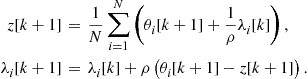
It is important to notice that, in this case, even if the global problem concerning the minimization of the augmented Lagrangian in (7.94) is certainly convex, the local problem in (7.95) is not necessarily convex because there is no guarantee that the term ![]() is a positive definite function. Nevertheless, the quadratic penalty present in (7.95) can make every local problem in (7.95) convex. At the same time, at convergence the penalty goes to zero and thus it does not induce any undesired bias on the final result.
is a positive definite function. Nevertheless, the quadratic penalty present in (7.95) can make every local problem in (7.95) convex. At the same time, at convergence the penalty goes to zero and thus it does not induce any undesired bias on the final result.
The first step in (7.95) can be made explicit, so that the algorithm assumes the form described in Table 7.6.
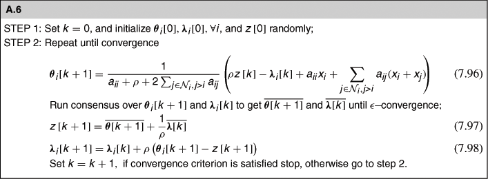
As an example, in Figure 7.12 we report the estimation versus the cumulative iteration index m that includes the consensus steps and the iterations over k. The results refer to a connected network with ![]() nodes;
nodes; ![]() has been chosen equal to 10 to guarantee that every local problem is convex. It can be noticed from Figure 7.12 that the distributed solution converges to the optimal centralized solution (horizontal x-marked line).
has been chosen equal to 10 to guarantee that every local problem is convex. It can be noticed from Figure 7.12 that the distributed solution converges to the optimal centralized solution (horizontal x-marked line).