

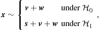
2.07.4.2 Decentralized observations with centralized estimation
In many cases, the observations are gathered in distributed form, through sensors deployed over a certain area, but the decision (either estimation or detection) is carried out in a central fusion center. In this section, we review some of the problems related to distributed estimation, with centralized decision. In such a case, the measurements gathered by the sensors are sent to a fusion center through rate-constrained physical channels. The question is how to design the quantization step in each sensor in order to optimize some performance metric related to the estimation of the parameter of interest. Let us start with an example, to introduce the basic issues.
Let us consider a network of N sensors, each observing a value ![]() containing a deterministic parameter
containing a deterministic parameter ![]() , corrupted by additive noise
, corrupted by additive noise ![]() , i.e.,
, i.e.,
![]() (7.99)
(7.99)
The noise variables ![]() are supposed to be zero mean spatially uncorrelated random variables with variance
are supposed to be zero mean spatially uncorrelated random variables with variance ![]() . Suppose that the sensors transmit their observations via some orthogonal multiple access scheme to a control center which wishes to estimate the unknown signal
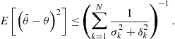
. Suppose that the sensors transmit their observations via some orthogonal multiple access scheme to a control center which wishes to estimate the unknown signal ![]() by minimizing the estimation mean square error (MSE)
by minimizing the estimation mean square error (MSE) ![]() . In the ideal case, where the observations are unquantized and received by the control center without distortion, the best linear unbiased estimator (BLUE) can be performed by the control center and the estimate
. In the ideal case, where the observations are unquantized and received by the control center without distortion, the best linear unbiased estimator (BLUE) can be performed by the control center and the estimate ![]() is given by
is given by
 (7.100)
with MSE given by ![]() . This estimator coincides with the maximum likelihood estimator when the noise variables are jointly Gaussian and uncorrelated.
. This estimator coincides with the maximum likelihood estimator when the noise variables are jointly Gaussian and uncorrelated.
Let us consider now the realistic case, where each sensor quantizes the observation ![]() to generate a discrete message
to generate a discrete message ![]() of
of ![]() bits. Assuming an error-free transmission, the fusion center must then provide an estimate
bits. Assuming an error-free transmission, the fusion center must then provide an estimate ![]() of the true parameter, based on the messages
of the true parameter, based on the messages ![]() transmitted by all the nodes. More specifically, assuming a uniform quantizer which generates unbiased message functions, the estimator at the control center performs a linear combination of the received messages. Let us suppose that the unknown signal to be estimated belongs to the range
transmitted by all the nodes. More specifically, assuming a uniform quantizer which generates unbiased message functions, the estimator at the control center performs a linear combination of the received messages. Let us suppose that the unknown signal to be estimated belongs to the range ![]() and each sensor uniformly divides the range
and each sensor uniformly divides the range ![]() into
into ![]() intervals of length
intervals of length ![]() rounding
rounding ![]() to the midpoint of these intervals. In this case, the quantized value
to the midpoint of these intervals. In this case, the quantized value ![]() at the kth sensor can be written as
at the kth sensor can be written as ![]() , where the quantization noise
, where the quantization noise ![]() is independent of
is independent of ![]() . It can be proved that
. It can be proved that ![]() is an unbiased estimator of
is an unbiased estimator of ![]() with
with
![]() (7.101)
(7.101)
where ![]() denotes an upper bound on the quantization noise variance and is given by
denotes an upper bound on the quantization noise variance and is given by
![]() (7.102)
(7.102)
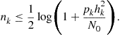
A linear unbiased estimator of ![]() is [49]
is [49]
 (7.103)
This estimate yields an MSE upper bound
 (7.104)
As mentioned before, the previous strategy assumes that there are no transmission errors. This property can be made as close as possible to reality by enforcing the transmission rate of sensor k to be strictly less than the channel capacity from sensor k to the fusion center. If we denote by ![]() the transmit power of sensor
the transmit power of sensor ![]() the channel coefficient between sensor k and control node and
the channel coefficient between sensor k and control node and ![]() is the noise variance at the control node receiver, the bound on transmit rate guaranteeing an arbitrarily small error probability is
is the noise variance at the control node receiver, the bound on transmit rate guaranteeing an arbitrarily small error probability is
 (7.105)
The problem is then how to allocate power and bits over each channel in order to fulfill some optimality criterion dictated by the estimation problem. This problem was tackled in [49] where it was proposed the minimization of the Euclidean norm of the transmit power vector under the constraint that the estimation variance is upper bounded by a given quantity and that the number of bits per symbol is less than the channel capacity. Here we formulate the problem as the minimization of the total transmit power under the constraint that the final MSE be upper bounded by a given quantity ![]() . From (7.105), defining
. From (7.105), defining ![]() , we can derive the number of quantization level as a function of the transmit power,6
, we can derive the number of quantization level as a function of the transmit power,6
![]() (7.106)
(7.106)
Our aim is to minimize the sum of powers transmitted by all the sensors under the constraint
 (7.107)
Denoting with ![]() the power vector, the optimization problem can be formulated as
the power vector, the optimization problem can be formulated as
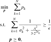 (7.108)
where ![]() is a function of
is a function of ![]() , as in (7.105). In practice, the values
, as in (7.105). In practice, the values ![]() are integer. However, searching for the optimal integer values
are integer. However, searching for the optimal integer values ![]() leads to an integer programming problem. To relax the problem, we assume that the variables
leads to an integer programming problem. To relax the problem, we assume that the variables ![]() are real. Then, by using (7.106), the optimization problem in (7.108) can be formulated as
are real. Then, by using (7.106), the optimization problem in (7.108) can be formulated as
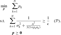 (7.109)
Problem ![]() is indeed a convex optimization problem and it is feasible if
is indeed a convex optimization problem and it is feasible if ![]() .
.
The optimal solution of the convex problem ![]() can be found by imposing the KKT conditions of
can be found by imposing the KKT conditions of ![]() , i.e.,
, i.e.,
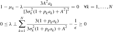 (7.110)
![]()
where ![]() and
and ![]() denote the Lagrangian multipliers associated to the
denote the Lagrangian multipliers associated to the ![]() constraints. The solution for the optimal powers turns out to be
constraints. The solution for the optimal powers turns out to be
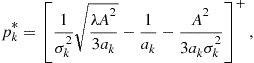 (7.111)
where ![]() and
and ![]() is found by imposing the MSE constraint to be valid with equality.
is found by imposing the MSE constraint to be valid with equality.
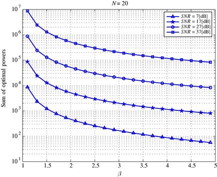
It is now useful to present some numerical results. To guarantee the existence of a solution, we set the bound ![]() with
with ![]() and
and ![]() . In Figure 7.13 we report the sum of the optimal transmit powers vs.
. In Figure 7.13 we report the sum of the optimal transmit powers vs. ![]() , for different SNR values. The number of sensors is
, for different SNR values. The number of sensors is ![]() . We can notice that the minimum transmit power increases for smaller values of
. We can notice that the minimum transmit power increases for smaller values of ![]() , i.e., when we require the realistic system to perform closer and closer to the ideal communication case.
, i.e., when we require the realistic system to perform closer and closer to the ideal communication case.
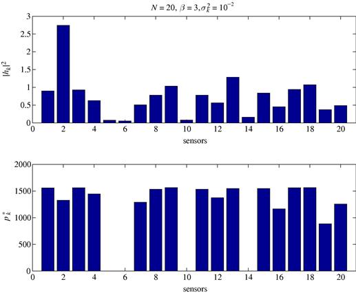
In the bottom subplot of Figure 7.14 we report an example of optimal power allocation obtained by solving the optimization problem ![]() , corresponding to the channel realization shown in the top subplot, assuming a constant observation noise variance
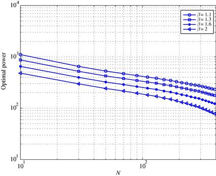
, corresponding to the channel realization shown in the top subplot, assuming a constant observation noise variance ![]() . We can observe that the solution is that only the nodes with the best channels coefficients are allowed to transmit. Finally, in Figure 7.15 we plot the sum of the optimal transmit powers versus the number of sensors N, for different values of
. We can observe that the solution is that only the nodes with the best channels coefficients are allowed to transmit. Finally, in Figure 7.15 we plot the sum of the optimal transmit powers versus the number of sensors N, for different values of ![]() . We can see that, as N increases, a lower power is necessary to achieve the desired estimation variance, as expected.
. We can see that, as N increases, a lower power is necessary to achieve the desired estimation variance, as expected.
2.07.5 Distributed detection
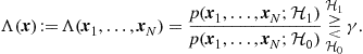
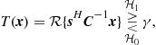
The distributed detection problem is in general more difficult to handle than the estimation problem. There is an extensive literature on distributed detection problem, but there is still a number of open problems. According to decision theory, an ideal centralized detector having error-free access to all the measurements collected by a set of nodes, should form the likelihood ratio and compare it with a suitable threshold [5]. Denoting with ![]() and
and ![]() the two alternative hypotheses, i.e., absence or presence of the event of interest, and with
the two alternative hypotheses, i.e., absence or presence of the event of interest, and with ![]() the joint probability density function of the whole set of observed data, under the hypothesis
the joint probability density function of the whole set of observed data, under the hypothesis ![]() , many decision tests can be cast as threshold strategies where the likelihood ratio (LR) is compared with a threshold
, many decision tests can be cast as threshold strategies where the likelihood ratio (LR) is compared with a threshold ![]() , which depends on the decision criterion. This is true, for example, for two important formulations leading to the Bayes approach and to the Neyman-Pearson criterion, the only difference between the two’s being the values assumed by the threshold
, which depends on the decision criterion. This is true, for example, for two important formulations leading to the Bayes approach and to the Neyman-Pearson criterion, the only difference between the two’s being the values assumed by the threshold ![]() . The detection rule decides for
. The detection rule decides for ![]() if the threshold is exceeded or for
if the threshold is exceeded or for ![]() , otherwise. In formulas,
, otherwise. In formulas,
 (7.112)
Ideally, with no communication constraints, every node should then send its observation vector ![]() , with
, with ![]() to the fusion center, which should then use all the received vectors to implement the LR test, as in (7.112). In reality, there are intrinsic limitations due to, namely: (a) the finite number of bits with which every sensor has to encode the measurements before transmission; (b) the maximum latency with which the decision has to be taken; (c) the finite capacity of the channel between sensors and fusion center. The challenging problem is then how to devise an optimum decentralized detection strategy taking into account the limitations imposed by the communication over realistic channels. The global problem, in the most general setting, is still an open problem, but there are many works in the literature addressing some specific cases. The interested reader may check the book [50] or the excellent tutorial reviews given in [51–53]. The situation becomes more complicated when we take explicitly into account the capacity bound imposed by the communication channel and we look for the number of bits to be used to quantize the local observations before transmitting to the fusion center. This problem was addressed in [54,55], where it was shown that binary quantization is optimal for the problem of detecting deterministic signals in Gaussian noise and for detecting signals in Gaussian noise using a square-law detector. The interesting indication, in these contexts, is that the gain offered by having more sensor nodes outperforms the benefits of getting more detailed (nonbinary) information from each sensor. A general framework to cast the problem of decentralized detection is the one where the topology describing the exchange of information among sensing nodes is not simply a tree, with all nodes sending data to a fusion center, but it is a graph. Each node is assumed to transmit a finite-alphabet symbol to its neighbors and the problem is how to find out the encoding (quantization) rule on each node. A class of problems admitting a message passing algorithm with provable convergence properties was proposed in [10]. The solution is a sort of distributed fusion protocol, taking explicitly into account the limits on the communication resources. An interesting and well motivated observation model is a correlated random field, as in many applications the observations concern physical quantities, like temperature or pressure, for example, which being subject to diffusion processes, are going to be spatially and temporally correlated. One of the first works addressing the detection of a known signal embedded in a correlated Gaussian noise was [56]. Using large deviations theory, the authors of [57] study the impact of node density, assuming that observations become increasingly correlated as sensors are in closer proximity of each other. More recently, the detection of a Gauss-Markov Random field (GMRF) with nearest-neighbor dependency was studied in [8]. Scaling laws for the energy consumption of optimal and sub-optimal fusion policies were then presented in [9]. The problem of energy-efficient routing of sensor observations from a Markov random field was analyzed in [58].
to the fusion center, which should then use all the received vectors to implement the LR test, as in (7.112). In reality, there are intrinsic limitations due to, namely: (a) the finite number of bits with which every sensor has to encode the measurements before transmission; (b) the maximum latency with which the decision has to be taken; (c) the finite capacity of the channel between sensors and fusion center. The challenging problem is then how to devise an optimum decentralized detection strategy taking into account the limitations imposed by the communication over realistic channels. The global problem, in the most general setting, is still an open problem, but there are many works in the literature addressing some specific cases. The interested reader may check the book [50] or the excellent tutorial reviews given in [51–53]. The situation becomes more complicated when we take explicitly into account the capacity bound imposed by the communication channel and we look for the number of bits to be used to quantize the local observations before transmitting to the fusion center. This problem was addressed in [54,55], where it was shown that binary quantization is optimal for the problem of detecting deterministic signals in Gaussian noise and for detecting signals in Gaussian noise using a square-law detector. The interesting indication, in these contexts, is that the gain offered by having more sensor nodes outperforms the benefits of getting more detailed (nonbinary) information from each sensor. A general framework to cast the problem of decentralized detection is the one where the topology describing the exchange of information among sensing nodes is not simply a tree, with all nodes sending data to a fusion center, but it is a graph. Each node is assumed to transmit a finite-alphabet symbol to its neighbors and the problem is how to find out the encoding (quantization) rule on each node. A class of problems admitting a message passing algorithm with provable convergence properties was proposed in [10]. The solution is a sort of distributed fusion protocol, taking explicitly into account the limits on the communication resources. An interesting and well motivated observation model is a correlated random field, as in many applications the observations concern physical quantities, like temperature or pressure, for example, which being subject to diffusion processes, are going to be spatially and temporally correlated. One of the first works addressing the detection of a known signal embedded in a correlated Gaussian noise was [56]. Using large deviations theory, the authors of [57] study the impact of node density, assuming that observations become increasingly correlated as sensors are in closer proximity of each other. More recently, the detection of a Gauss-Markov Random field (GMRF) with nearest-neighbor dependency was studied in [8]. Scaling laws for the energy consumption of optimal and sub-optimal fusion policies were then presented in [9]. The problem of energy-efficient routing of sensor observations from a Markov random field was analyzed in [58].
A classification of the various detection algorithms depends on the adopted criterion. A first important classification is the following:
1. Global decision is taken at the fusion center
a. Nodes send data to FC; FC takes global decision
b. Nodes send local decisions to FC; FC fuses local decisions
2. Every node is able to take a global decision
In the first case, the observation is distributed across the nodes, but the decision is centralized. This case has received most of the attention. The interested reader may check, for example, the book [50] or the tutorial reviews given in [51–53]. In the second case, also the decision is decentralized. This case has been considered only relatively recently. Some references are, for example, [59–65].
An alternative classification is between
In the first case, the network collects a given amount of data along the time and space domains and then it takes a decision. In the second case, the number of observations, either in time or in terms of number of involved sensors, is not decided a priori, but it is updated at every new measurement. The network stops collecting information only when some performance criterion is satisfied (typically, false alarm and detection probability) [66–68].
One of the major difficulties in distributed detection comes from establishing the optimal decision thresholds at local and global level. The main problem is how to optimize the local decisions, taking into account that the final decisions will be only the result of the interaction among the nodes. Taking a local decision can be interpreted as a form of source coding. The simple (binary) hypothesis testing can be seen in fact as a form of binary coding. Whenever the observations are conditionally independent, given each hypothesis, the likelihood ratio test at the sensor nodes is indeed optimal [69]. However, finding the optimal quantization levels is a difficult task. Even when the observations are i.i.d., assuming identical decision rules is very common and apparently well justified. Nevertheless there are counterexamples showing that nonidentical decision rules are optimal [69]. Identical decision rules in the i.i.d. case turns out to be optimal only asymptotically, as the number of nodes tends to infinity [70].
A simple example may be useful to grasp some of the difficulties associated with distributed detection. For this purpose, we briefly recall the seminal work of Tenney and Sandell [71]. Let us consider two sensors, each measuring a real quantity ![]() , with
, with ![]() . Based on its observation
. Based on its observation ![]() , sensor i decides whether the phenomenon of interest is present or not. In the first case, it sets the decision variable
, sensor i decides whether the phenomenon of interest is present or not. In the first case, it sets the decision variable ![]() , otherwise, it sets
, otherwise, it sets ![]() . The question is how to implement the decision strategy, according to some optimality criterion. The approach proposed in [71] is a Bayesian approach, where the goal of each sensor is to minimize the Bayes risk, which can be made explicit by introducing the cost coefficients and the observation probability model. Let us denote by
. The question is how to implement the decision strategy, according to some optimality criterion. The approach proposed in [71] is a Bayesian approach, where the goal of each sensor is to minimize the Bayes risk, which can be made explicit by introducing the cost coefficients and the observation probability model. Let us denote by ![]() the cost of detector 1 deciding on
the cost of detector 1 deciding on ![]() , detector 2 deciding on
, detector 2 deciding on ![]() , when the true hypothesis is
, when the true hypothesis is ![]() . Denoting by
. Denoting by ![]() the prior probability of event
the prior probability of event ![]() and by
and by ![]() the joint pdf of having
the joint pdf of having ![]() , observing the pair
, observing the pair ![]() and deciding for the pair
and deciding for the pair ![]() , the average risk can be written as
, the average risk can be written as
 (7.113)
In this case, each node observes only its own variable and takes a decision independently of the other node. Hence, we can set
![]() (7.114)
(7.114)
Expanding the right hand side by explicitly summing over index i, we get
![]() (7.115)
(7.115)
Considering that ![]() and ignoring all terms which do not contain
and ignoring all terms which do not contain ![]() , we get
, we get
![]() (7.116)
(7.116)
The average risk is minimized if ![]() is chosen as follows
is chosen as follows
 (7.117)
This expression shows that the optimal local decision rule is a deterministic rule. After a few algebraic manipulations, (7.117) can be rewritten, equivalently, as [50]
 (7.118)
where ![]() is the LR at node 1. Eq. (7.118) has the structure of a LRT. However, note that the threshold on the right hand side of (7.118) depends on the observation
is the LR at node 1. Eq. (7.118) has the structure of a LRT. However, note that the threshold on the right hand side of (7.118) depends on the observation ![]() , through the term
, through the term ![]() , which incorporates the statistical dependency between the observations
, which incorporates the statistical dependency between the observations ![]() and
and ![]() . Hence, Eq. (7.118) is not a proper LRT.
. Hence, Eq. (7.118) is not a proper LRT.
The situation simplifies if the observations are conditionally independent, i.e., ![]() . In such a case, the threshold
. In such a case, the threshold ![]() can be simplified into
can be simplified into
![]() (7.119)
(7.119)
Since ![]() , (7.119) can be rewritten as
, (7.119) can be rewritten as
![]() (7.120)
(7.120)
Hence, the threshold ![]() to be used at node 1 is a function of
to be used at node 1 is a function of ![]() , i.e., on the decision taken by node 2. At the same time, the threshold
, i.e., on the decision taken by node 2. At the same time, the threshold ![]() to be used by node 2 will depend on the decision rule followed by node 1. This means that, even if the observations are conditionally independent and the decisions are taken autonomously by the two nodes, the decisions are still coupled through the thresholds. This simple example shows how the detection problem can be rather complicated, even under a very simple setting.
to be used by node 2 will depend on the decision rule followed by node 1. This means that, even if the observations are conditionally independent and the decisions are taken autonomously by the two nodes, the decisions are still coupled through the thresholds. This simple example shows how the detection problem can be rather complicated, even under a very simple setting.
In the special case where ![]() ,
, ![]() , and
, and ![]() , i.e., there is no penalty if the decisions are correct, the penalty is 1, when there is one error, and the penalty is 2 when there are two errors, the threshold simplifies into
, i.e., there is no penalty if the decisions are correct, the penalty is 1, when there is one error, and the penalty is 2 when there are two errors, the threshold simplifies into
![]() (7.121)
(7.121)
Hence, in this special case, the two thresholds are independent of each other and the two detectors become independent of each other.
After having pointed out through a simple example some of the problems related to distributed detection, it is now time to consider in more detail the cases where the nodes send their (possibly encoded) data to the FC or they take local decisions first and send them to the FC. In both situations, there are two extreme cases: (a) there is only one FC; (b) every node is a potential FC, as it is able to take a global decision.
2.07.5.1 Nodes send data to decision center
Let us consider for simplicity the simple (binary) hypothesis testing problem. Given a set of vector observations ![]() , where
, where ![]() is the vector collected by node
is the vector collected by node ![]() , the optimal decision rule for the simple hypothesis testing problem, under a variety of optimality criteria, amounts to compute the likelihood ratio (LR)
, the optimal decision rule for the simple hypothesis testing problem, under a variety of optimality criteria, amounts to compute the likelihood ratio (LR) ![]() and compare it with a threshold. In formulas,
and compare it with a threshold. In formulas,
 (7.122)
In words, the detector decides for ![]() if the LR exceeds the threshold, otherwise it decides for
if the LR exceeds the threshold, otherwise it decides for ![]() . In general, what changes the distributed detection problem from the standard centralized detection is that the data are sent to the decision center after source encoding into a discrete alphabet. The simplest form of encoding is quantization. But also taking local decisions can be interpreted as a form of binary coding. Clearly, source coding is going to affect the detection performance. It is then useful to show, through a simple example, how local quantization affects the final detection performance and how we can benefit from the theoretical analysis to optimize the number of bits associated to the quantization step in order to optimize performance of the detection scheme.
. In general, what changes the distributed detection problem from the standard centralized detection is that the data are sent to the decision center after source encoding into a discrete alphabet. The simplest form of encoding is quantization. But also taking local decisions can be interpreted as a form of binary coding. Clearly, source coding is going to affect the detection performance. It is then useful to show, through a simple example, how local quantization affects the final detection performance and how we can benefit from the theoretical analysis to optimize the number of bits associated to the quantization step in order to optimize performance of the detection scheme.
2.07.5.1.1 Centralized detection of deterministic signal embedded in additive noise
Let us consider the detection of a deterministic (known) signal embedded in additive noise. In this section, we consider the case where the decision is taken at a FC, after having collected the data sent by the sensors. This case could refer for example to the detection of undesired resonance phenomena in buildings, bridges, etc. The form of the resonance is known. However, the measurements taken by the sensors are affected by noise and then it is of interest to check the performance as a function of the signal to noise ratio.
The measurement vector is ![]() , where
, where ![]() is the measurement taken by node i. Let us denote as
is the measurement taken by node i. Let us denote as ![]() the known deterministic signal. The observation can be modeled as
the known deterministic signal. The observation can be modeled as
 (7.123)
where ![]() is the background noise, whereas
is the background noise, whereas ![]() is the quantization noise. We assume the noise to be Gaussian with zero mean and (spatial) covariance matrix
is the quantization noise. We assume the noise to be Gaussian with zero mean and (spatial) covariance matrix ![]() , i.e.,
, i.e., ![]() . To simplify the mathematical tractability, we consider a dithered quantization so that the quantization error can be modeled as a random process statistically independent of noise. We may certainly assume that, after dithering, the quantization noise variables over different sensors are statistically independent. Hence, we can state that the quantization noise vector
. To simplify the mathematical tractability, we consider a dithered quantization so that the quantization error can be modeled as a random process statistically independent of noise. We may certainly assume that, after dithering, the quantization noise variables over different sensors are statistically independent. Hence, we can state that the quantization noise vector ![]() has zero mean and a diagonal covariance matrix
has zero mean and a diagonal covariance matrix ![]() . If the amplitude of the useful signal spans the dynamic range
. If the amplitude of the useful signal spans the dynamic range ![]() and the number of bits used by node i is
and the number of bits used by node i is ![]() , the quantum range is
, the quantum range is ![]() so that the quantization noise variance at node i is
so that the quantization noise variance at node i is
![]() (7.124)
(7.124)
The overall noise has then a zero mean and covariance matrix ![]() .
.
If the quantization noise is negligible, the Neyman-Pearson criterion applied to this case leads to the following linear detector
 (7.125)
where ![]() denotes the real part of x, and the detection threshold
denotes the real part of x, and the detection threshold ![]() is computed in order to guarantee the desired false alarm probability
is computed in order to guarantee the desired false alarm probability ![]() . Unfortunately, since the quantization noise is not Gaussian, the composite noise
. Unfortunately, since the quantization noise is not Gaussian, the composite noise ![]() is not Gaussian and then the detection rule in (7.125) is no longer optimal. Nevertheless, the rule in (7.125) is still meaningful as it maximizes the signal to noise ratio (SNR). Hence, it is of interest to look at the performance of this detector in the presence of quantization noise. The exact computation of the detection probability is not easy, at least in closed form, because it requires the computation of the pdf of
is not Gaussian and then the detection rule in (7.125) is no longer optimal. Nevertheless, the rule in (7.125) is still meaningful as it maximizes the signal to noise ratio (SNR). Hence, it is of interest to look at the performance of this detector in the presence of quantization noise. The exact computation of the detection probability is not easy, at least in closed form, because it requires the computation of the pdf of ![]() . Nevertheless, when the number of nodes is sufficiently high (an order of a few tens can be sufficient to get a good approximation), we can invoke the central limit theorem to state that
. Nevertheless, when the number of nodes is sufficiently high (an order of a few tens can be sufficient to get a good approximation), we can invoke the central limit theorem to state that ![]() is approximately Gaussian. Using this approximation, the detection probability can be written in closed form for any fixed
is approximately Gaussian. Using this approximation, the detection probability can be written in closed form for any fixed ![]() , following standard derivations (see, e.g., [5]), as
, following standard derivations (see, e.g., [5]), as
![]() (7.126)
(7.126)
This formula is useful to assess the detection probability as a function of the bits allocated to each transmission. At the same time, we can also use (7.126) as a way to find out the bit allocation that maximizes the detection probability. This approach establishes an interesting link between the communication and detection aspects. In practice, in fact, encoded data are transmitted over a finite capacity channel. Hence, it is useful to relate the number of quantization bits used by each node and capacity of the channel between that node and the FC. For simplicity, we consider the optimization problem under the assumption of spatially uncorrelated noise, i.e., ![]() . The problem we wish to solve is the maximization of the detection probability, for a given false alarm rate and a maximum global transmit power. To guarantee an arbitrarily low transmission error rate, we need to respect Shannon’s channel coding theorem, so that the number of bits per symbol must be less than channel capacity. Denoting with
. The problem we wish to solve is the maximization of the detection probability, for a given false alarm rate and a maximum global transmit power. To guarantee an arbitrarily low transmission error rate, we need to respect Shannon’s channel coding theorem, so that the number of bits per symbol must be less than channel capacity. Denoting with ![]() the power transmitted by user i and assuming flat fading channel, with channel coefficient
the power transmitted by user i and assuming flat fading channel, with channel coefficient ![]() , the capacity is given by (7.105). From(7.126), maximizing
, the capacity is given by (7.105). From(7.126), maximizing ![]() is equivalent to maximizing
is equivalent to maximizing ![]() . Hence, using (7.124), the maximum
. Hence, using (7.124), the maximum ![]() , for a given
, for a given ![]() and a given global transmit power
and a given global transmit power ![]() , can be achieved by finding the power vector
, can be achieved by finding the power vector ![]() that solves the following constrained problem
that solves the following constrained problem
 (7.127)
 (7.128)
It is straightforward to check that this is a convex problem. Imposing the Karush-Kuhn-Tucker conditions, the optimal powers can be expressed in closed form as:
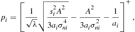 (7.129)
where the Lagrange multiplier ![]() associated to the sum-power constraint can be determined as the value that makes
associated to the sum-power constraint can be determined as the value that makes ![]() .
.
A numerical example is useful to grasp some of the properties of the proposed algorithm. Let us consider a series of sensors placed along a bridge of length L. The purpose of the network is to detect one possible spatial resonance, which we represent as the signal ![]() , where
, where ![]() denotes the spatial coordinate. The sensors are uniformly spaced along the bridge, at positions
denotes the spatial coordinate. The sensors are uniformly spaced along the bridge, at positions ![]() , with
, with ![]() . Every sensor measures a shift
. Every sensor measures a shift ![]() , affected by the error
, affected by the error ![]() . To communicate its own measurement to the FC, every sensor has to quantize the measurement first. The optimal number of bits to be used by every sensor can be computed by using the previous theory. In this case, in Figure 7.16 we report the detection probability vs. the sum power
. To communicate its own measurement to the FC, every sensor has to quantize the measurement first. The optimal number of bits to be used by every sensor can be computed by using the previous theory. In this case, in Figure 7.16 we report the detection probability vs. the sum power ![]() available to the whole set of sensors, for different numbers N of sensors. As expected, as the total transmit power increases,
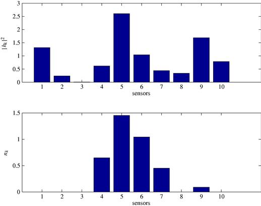
available to the whole set of sensors, for different numbers N of sensors. As expected, as the total transmit power increases, ![]() increases because more bits per symbol can be transmitted and then the quantization errors become negligible. It is also important to notice how, increasing the number of sensors, the detection probability improves, for any given transmit power. Furthermore, in Figure 7.17 we can see the optimal per channel bit allocation (bottom), together with the channels profiles
increases because more bits per symbol can be transmitted and then the quantization errors become negligible. It is also important to notice how, increasing the number of sensors, the detection probability improves, for any given transmit power. Furthermore, in Figure 7.17 we can see the optimal per channel bit allocation (bottom), together with the channels profiles ![]() (top). Interestingly, we can see that the method allocates more bits in correspondence with the best channels and the central elements of the array, where the useful signal is expected to have the largest variations.
(top). Interestingly, we can see that the method allocates more bits in correspondence with the best channels and the central elements of the array, where the useful signal is expected to have the largest variations.

2.07.5.1.2 Decentralized detection under conditionally independent observations
Let us consider now the case where the globally optimal decision can be taken, in principle, by any node. To enable this possibility, every node must be able to implement the statistical test (7.122). If the measurements collected by the sensors are conditionally independent, the logarithm of the likelihood ratio can be written as
 (7.130)
This formula shows that, in the conditionally independent case, running a consensus algorithm is sufficient to enable every node to compute the global LR. It is only required that every sensor initializes its own state with the local log-LR ![]() and then runs the consensus iterations. If the network is connected, every node will end up with the average value of the local LR’s. In practice, to send the local LR, every node must quantize it first. Then, we need to refer to the consensus algorithm in the presence of quantization errors. However, we have already seen in Section 2.07.3.2 that the consensus iterations may be properly modified to make the algorithm robust against a series of drawbacks coming from communications through realistic channels, as, eg., random packet drops and quantization. Hence, a consensus algorithm, properly modified, can enable every node to compute the global LR with controllable error.
and then runs the consensus iterations. If the network is connected, every node will end up with the average value of the local LR’s. In practice, to send the local LR, every node must quantize it first. Then, we need to refer to the consensus algorithm in the presence of quantization errors. However, we have already seen in Section 2.07.3.2 that the consensus iterations may be properly modified to make the algorithm robust against a series of drawbacks coming from communications through realistic channels, as, eg., random packet drops and quantization. Hence, a consensus algorithm, properly modified, can enable every node to compute the global LR with controllable error.
2.07.5.2 Nodes send local decisions to fusion center
Consider now the case where each node i takes a local decision, according to a locally optimal criterion, and encodes the decision into the binary variable ![]() . Then, the node sends the variable
. Then, the node sends the variable ![]() to the fusion center, which is asked to take a global decision on the basis of the vector
to the fusion center, which is asked to take a global decision on the basis of the vector ![]() containing all local decisions. Let us consider for simplicity the binary hypothesis test. This problem was considered in [50] and we will now review the basic results. This problem is distinct from the case studied in the previous section because here the local decision thresholds are optimized according to a detection criterion, whereas in standard quantization the decision thresholds are not optimized.
containing all local decisions. Let us consider for simplicity the binary hypothesis test. This problem was considered in [50] and we will now review the basic results. This problem is distinct from the case studied in the previous section because here the local decision thresholds are optimized according to a detection criterion, whereas in standard quantization the decision thresholds are not optimized.
Under both Bayesian and Neyman-Pearson (NP) formulations, the optimal test amounts to a likelihood ratio test, based on ![]() , i.e.,
, i.e.,
![]() (7.131)
(7.131)
In the case of conditionally independent local decisions, the LRT converts into
 (7.132)
Since each variable ![]() can only assume the values 0 or 1, we can group all the variables into two subsets: the subset
can only assume the values 0 or 1, we can group all the variables into two subsets: the subset ![]() containing all variables
containing all variables ![]() and the subset
and the subset ![]() containing all variables
containing all variables ![]() , thus yielding
, thus yielding
![]() (7.133)
(7.133)
Denoting with ![]() , and
, and ![]() , the probabilities of miss and the probability of false alarm of node i, respectively, (7.133) can be rewritten as
, the probabilities of miss and the probability of false alarm of node i, respectively, (7.133) can be rewritten as
![]() (7.134)
(7.134)
Taking the logarithm of both sides and reintroducing the variables ![]() , the fusion rule becomes
, the fusion rule becomes
 (7.135)
or, equivalently
 (7.136)
The optimal fusion rule is then a simple weighted sum of the local decisions, where the weights depend on the reliabilities of the local decisions: Larger weights are assigned to the most reliable nodes.
If instead of having a single FC, we wish to enable every node to implement the decision fusion rule described above, we can see that, again, running a consensus algorithm suffices to reach the goal. In fact, if each local state variable is initialized with a value ![]() , running a consensus algorithm allows every node to know the function in (7.136). The only constraint is, as always, network connectivity. The drawback of this simple approach is that running this sort of consensus algorithm requires the transmission of real variables, rather than the binary variables
, running a consensus algorithm allows every node to know the function in (7.136). The only constraint is, as always, network connectivity. The drawback of this simple approach is that running this sort of consensus algorithm requires the transmission of real variables, rather than the binary variables ![]() . In fact, even if the local decision
. In fact, even if the local decision ![]() is binary, the coefficient multiplying
is binary, the coefficient multiplying ![]() is a real variable, which needs to be quantized before transmission over a realistic channel. Again, the consensus algorithm can be robustified against quantization errors by using dithered quantization and a decreasing step size, as shown in 2.07.3.2. However, it is important to clarify that we cannot make any claim of optimality of this kind of distributed decision. In principle, when the nodes exchange their decisions with the neighbors, the decision thresholds should be adjusted in order to accommodate some optimality criterion. This is indeed an interesting, yet still open, research topic.
is a real variable, which needs to be quantized before transmission over a realistic channel. Again, the consensus algorithm can be robustified against quantization errors by using dithered quantization and a decreasing step size, as shown in 2.07.3.2. However, it is important to clarify that we cannot make any claim of optimality of this kind of distributed decision. In principle, when the nodes exchange their decisions with the neighbors, the decision thresholds should be adjusted in order to accommodate some optimality criterion. This is indeed an interesting, yet still open, research topic.
2.07.6 Beyond consensus: distributed projection algorithms
In many applications, the field to be reconstructed by a sensor network is typically a smooth function of the spatial coordinates. This happens for example, in the reconstruction of the spatial distribution of the power radiated by a set of transmitters. The problem is that local measurements may be corrupted by local noise or fading effects. An important application of this scenario is given by cognitive networks. In such a case, a secondary node would need to know the channel occupation across space, to find out unoccupied channels, within the area of interest. This requires some sort of spectrum sensing, but in a localized area. The problem of sensing is that wireless propagation is typically affected by fading or shadowing effects, so that a sensor in a shadowed location might indicate that a channel is unoccupied, while this is not true. To avoid this kind of error, which would lead to undue channel occupation from opportunistic users, it is useful to resort to cooperative sensing. In such a case, nearby nodes exchange local measurements to counteract the effect of shadowing.
The problem with local averaging operations is that they should reduce the effect of fading, but without destroying valuable spatial variations. In the following, we recall a distributed algorithm proposed in [72] to recover a spatial map of a field, using local weighted averages where the weights are chosen so as to improve upon local noise or fading effects, but without destroying the spatial variation of the useful signal.
Let us consider a network composed of N sensors located at positions ![]() , and denote the measurement collected by the ith sensor by
, and denote the measurement collected by the ith sensor by ![]() , where
, where ![]() represents the useful field while
represents the useful field while ![]() is the observation error. Let us also denote by
is the observation error. Let us also denote by ![]() , a set of linearly independent spatial functions defining a basis for the useful signal. The useful signal can then be represented through the basis expansion model
, a set of linearly independent spatial functions defining a basis for the useful signal. The useful signal can then be represented through the basis expansion model
![]() (7.137)
(7.137)
In vector notation, introducing the N-size column vector ![]() and similarly for the vector
and similarly for the vector ![]() , we may write
, we may write
![]() (7.138)
(7.138)
where ![]() is the
is the ![]() matrix whose mth column is
matrix whose mth column is ![]() ,
, ![]() is an r-size vector of coefficients and
is an r-size vector of coefficients and ![]() is the useful signal. The spatial smoothness of the useful signal field may be captured by choosing the functions
is the useful signal. The spatial smoothness of the useful signal field may be captured by choosing the functions ![]() to be the low frequency components of the Fourier basis or low-order 2 D polynomials. For instance, if the space under monitoring is a square of side L, we may choose the set
to be the low frequency components of the Fourier basis or low-order 2 D polynomials. For instance, if the space under monitoring is a square of side L, we may choose the set
![]() (7.139)
(7.139)
In practice, the dimension r of the useful signal subspace is typically much smaller than the dimension N of the observation space, i.e., of the number of sensors. We can exploit this property to devise a distributed denoising algorithm.
If we use a Minimum Mean Square Error (MMSE) strategy, the goal is to find the useful signal vector ![]() that minimizes the mean square error
that minimizes the mean square error
![]() (7.140)
(7.140)
The solution is well known and is given by [44]:
![]() (7.141)
(7.141)
Our goal is actually to recover the vector ![]() , rather than
, rather than ![]() . In such a case, the estimate of
. In such a case, the estimate of ![]() is
is
![]() (7.142)
(7.142)
The operation performed in (7.142) corresponds to projecting the observation vector onto the subspace spanned by the columns of ![]() . Assuming, without any loss of generality (w.l.o.g.), the columns of
. Assuming, without any loss of generality (w.l.o.g.), the columns of ![]() to be orthonormal, the projector simplifies into
to be orthonormal, the projector simplifies into
![]() (7.143)
(7.143)
The centralized solution to this problem is then very simple: The fusion center collects all the measurements ![]() , compute
, compute ![]() and then recovers
and then recovers ![]() from (7.143).
from (7.143).
The previous approach is well known. The interesting point is that the MMSE solution can be achieved with a totally decentralized approach, where every sensor interacts only with its neighbors, with no need to send any data to a fusion center. The proposed approach is based on a very simple iterative procedure, where each node initializes a state variable with the local measurement, let us say ![]() , and then it updates its own state by taking a linear combination of its neighbors’ states, similarly with what happens with consensus algorithms, but with coefficients computed in order to solve the new problem.
, and then it updates its own state by taking a linear combination of its neighbors’ states, similarly with what happens with consensus algorithms, but with coefficients computed in order to solve the new problem.
More specifically, denoting by ![]() , the N-size vector containing the states of all the nodes, at iteration k, and by
, the N-size vector containing the states of all the nodes, at iteration k, and by ![]() the vector containing the initial measurements collected by all the nodes, the vector
the vector containing the initial measurements collected by all the nodes, the vector ![]() evolves according to the following linear state equation:
evolves according to the following linear state equation:
![]() (7.144)
(7.144)
where ![]() is typically a sparse (not necessarily symmetric) matrix. The network topology is reflected into the sparsity of
is typically a sparse (not necessarily symmetric) matrix. The network topology is reflected into the sparsity of ![]() . In particular, the number of nonzero entries of, let us say, the ith row is equal to the number of neighbors of node i. In a WSN, the neighbors of a node are the nodes falling within the coverage area of that node, i.e., within a circle centered on the location of the node, with radius dictated by the transmit power of the node and by the power attenuation law. Our goal is to find the nonnull coefficients of
. In particular, the number of nonzero entries of, let us say, the ith row is equal to the number of neighbors of node i. In a WSN, the neighbors of a node are the nodes falling within the coverage area of that node, i.e., within a circle centered on the location of the node, with radius dictated by the transmit power of the node and by the power attenuation law. Our goal is to find the nonnull coefficients of ![]() that allow the convergence of
that allow the convergence of ![]() to the vector
to the vector ![]() given in (7.143). In general, not every network topology guarantees the existence of a solution of this problem. In the following, we will show that a solution exists only if each node has a number of neighbors greater than the dimension r of the useful signal subspace.
given in (7.143). In general, not every network topology guarantees the existence of a solution of this problem. In the following, we will show that a solution exists only if each node has a number of neighbors greater than the dimension r of the useful signal subspace.
Let us denote by ![]() the orthogonal projector onto the r-dimensional subspace of
the orthogonal projector onto the r-dimensional subspace of ![]() spanned by the columns of
spanned by the columns of ![]() , where
, where ![]() denotes the range space operator and
denotes the range space operator and ![]() is a full-column rank matrix, assumed, w.l.o.g., to be semi-unitary. System (7.144) converges to the desired orthogonal projection of the initial value vector
is a full-column rank matrix, assumed, w.l.o.g., to be semi-unitary. System (7.144) converges to the desired orthogonal projection of the initial value vector ![]() onto
onto ![]() , for any given
, for any given ![]() , if and only if
, if and only if
![]() (7.145)
(7.145)
i.e.,
![]() (7.146)
(7.146)
Resorting to basic algebraic properties of discrete-time systems, it is possible to derive immediately some basic properties of ![]() . In particular, denoting with OUD the Open Unit Disk, i.e., the set
. In particular, denoting with OUD the Open Unit Disk, i.e., the set ![]() , a matrix
, a matrix ![]() is semistable if its spectrum
is semistable if its spectrum ![]() satisfies
satisfies ![]() and, if
and, if ![]() , then 1 is semisimple, i.e., its algebraic and geometric multiplicities coincide. If
, then 1 is semisimple, i.e., its algebraic and geometric multiplicities coincide. If ![]() is semistable, then [73, p.447]
is semistable, then [73, p.447]
![]() (7.147)
(7.147)
where ![]() denotes group generalized inverse [73, p.228]. Furthermore, setting, without loss of generality, the matrix
denotes group generalized inverse [73, p.228]. Furthermore, setting, without loss of generality, the matrix ![]() in the form
in the form ![]() , (7.147) can be rewritten as
, (7.147) can be rewritten as
![]() (7.148)
(7.148)
But ![]() is the projector onto the null-space of
is the projector onto the null-space of ![]() . Hence, we can state the following:
. Hence, we can state the following:
Proposition 1
Given the dynamical system in (7.144) and the projection matrix![]() , the vector
, the vector![]() is globally asymptotically stable for any fixed
is globally asymptotically stable for any fixed![]() , if and only if the following conditions are satisfied:
, if and only if the following conditions are satisfied:
Alternatively, the previous conditions can be rewritten equivalently in the following form
Proposition 2
Given the dynamical system in(7.144)and the projection matrix![]() , the vector
, the vector![]() is globally asymptotically stable for any fixed
is globally asymptotically stable for any fixed![]() , if and only if the following conditions are satisfied:
, if and only if the following conditions are satisfied:
![]() (C.1)
(C.1)
![]() (C.2)
(C.2)
![]() (C.3)
(C.3)
where![]() denotes the spectral radius operator[23].
denotes the spectral radius operator[23].
Remark 1
Conditions (C.1)–(C.3) have an intuitive interpretation. In particular, C.1 and C.2 state that, if system (7.144) asymptotically converges, then it is guaranteed to converge to the desired value. In fact, C.1 guarantees that the projection of vector ![]() onto
onto ![]() is an invariant quantity for the dynamical system, implying that the system in (7.144), during its evolution, keeps the component
is an invariant quantity for the dynamical system, implying that the system in (7.144), during its evolution, keeps the component ![]() of
of ![]() unaltered. At the same time, C.2 makes
unaltered. At the same time, C.2 makes ![]() a fixed point of matrix
a fixed point of matrix ![]() and thus a potential accumulation point for the sequence
and thus a potential accumulation point for the sequence ![]() . Both conditions C.1 and C.2 do not state anything about the convergence of the dynamical system. This is guaranteed by C.3, which imposes that all the modes associated to the eigenvectors orthogonal to
. Both conditions C.1 and C.2 do not state anything about the convergence of the dynamical system. This is guaranteed by C.3, which imposes that all the modes associated to the eigenvectors orthogonal to ![]() are asymptotically vanishing.
are asymptotically vanishing.
Remark 2
The conditions (C.1)–(C.3) contain, as a special case, the convergence conditions of average consensus algorithm. In fact, it is sufficient to set in (7.145), ![]() and
and ![]() , where
, where ![]() is the N-length vector of all ones. In such a case, (C.1)–(C.3) can be restated as following: the digraph associated to the network described by
is the N-length vector of all ones. In such a case, (C.1)–(C.3) can be restated as following: the digraph associated to the network described by ![]() must be strongly connected and balanced.
must be strongly connected and balanced.
The previous conditions do not make any explicit reference to the sparsity of matrix ![]() . However, when we consider a sparse matrix, reflecting the network topology, additional conditions are necessary to make sure that the previous conditions are satisfied. In other words, not every network topology is able to guarantee the asymptotic projection onto a prescribed signal subspace. One basic question is then what network topology is able to guarantee the convergence to a prescribed projector. We provide now the conditions on the sparsity of
. However, when we consider a sparse matrix, reflecting the network topology, additional conditions are necessary to make sure that the previous conditions are satisfied. In other words, not every network topology is able to guarantee the asymptotic projection onto a prescribed signal subspace. One basic question is then what network topology is able to guarantee the convergence to a prescribed projector. We provide now the conditions on the sparsity of ![]() , or equivalently
, or equivalently ![]() , guaranteeing the desired convergence.
, guaranteeing the desired convergence.
From condition (i) of Proposition 1, given the matrix ![]() ,
, ![]() must satisfy the equation
must satisfy the equation ![]() . Let us assume that every row of
. Let us assume that every row of ![]() has K nonzero entries and let us indicate with
has K nonzero entries and let us indicate with ![]() the set of the column indices corresponding to the nonzero entries of the jth row of
the set of the column indices corresponding to the nonzero entries of the jth row of ![]() . Hence, every row of
. Hence, every row of ![]() must satisfy the following equation
must satisfy the following equation
 (7.149)
To guarantee the existence of a nontrivial solution to (7.149), the matrix on the left hand side must have a kernel of dimension at least one. This requires K to be strictly greater than r, the dimension of the signal subspace. Since the number of nonzero entries of, let us say the jth, row of ![]() is equal to the number of neighbors of node j plus one (the coefficient multiplying the state of node i itself), this implies that the minimum number K of neighbors of each node must be at least equal to the dimension r of the signal subspace. Of course this condition is necessary but not sufficient. It is also necessary to check that the sparse matrix
is equal to the number of neighbors of node j plus one (the coefficient multiplying the state of node i itself), this implies that the minimum number K of neighbors of each node must be at least equal to the dimension r of the signal subspace. Of course this condition is necessary but not sufficient. It is also necessary to check that the sparse matrix ![]() built with rows satisfying (7.149), with
built with rows satisfying (7.149), with ![]() , had rank
, had rank ![]() . This depends on the location of the nodes and on the specific choice of the orthogonal basis.
. This depends on the location of the nodes and on the specific choice of the orthogonal basis.
An example can be useful to illustrate the benefits achievable with the proposed technique. We consider the case where the observation is corrupted by a multiplicative, spatially uncorrelated, noise, which models, for example a fading effect. Let us denote with ![]() the measurement carried out from node i, located in the point of coordinates
the measurement carried out from node i, located in the point of coordinates ![]() , where
, where ![]() denotes the useful field, whereas
denotes the useful field, whereas ![]() represents fading. We consider, for instance, a useful signal composed by
represents fading. We consider, for instance, a useful signal composed by ![]() transmitters and we assume a polynomial power attenuation, so that the useful signal measured at the point of coordinates
transmitters and we assume a polynomial power attenuation, so that the useful signal measured at the point of coordinates ![]() is
is
 (7.150)
where ![]() is the power emitted by source i, located at
is the power emitted by source i, located at ![]() , and
, and ![]() specifies the power spatial spread. Furthermore, fading is modeled as a spatially uncorrelated multiplicative noise. The sensor network is composed of 2500 nodes uniformly distributed over a 2D grid. All the transmitters use the same power, i.e.,
specifies the power spatial spread. Furthermore, fading is modeled as a spatially uncorrelated multiplicative noise. The sensor network is composed of 2500 nodes uniformly distributed over a 2D grid. All the transmitters use the same power, i.e., ![]() in (7.150), and the noise has zero mean and variance
in (7.150), and the noise has zero mean and variance ![]() .
.
In this case, it is useful to apply a homomorphic filtering to the measured field. In particular, we take the ![]() of the measurement, thus getting
of the measurement, thus getting ![]() . To smooth out the undesired effect of fading, we assume a signal model composed by the superposition of 2D sinusoids, so that the columns of the matrix
. To smooth out the undesired effect of fading, we assume a signal model composed by the superposition of 2D sinusoids, so that the columns of the matrix ![]() in (7.138) are composed of signals of the form
in (7.138) are composed of signals of the form ![]() , and
, and ![]() , with
, with ![]() . We set the initial value of the state of each node equal to
. We set the initial value of the state of each node equal to ![]() and we run the distributed projection algorithm described above. After convergence, we simply take the
and we run the distributed projection algorithm described above. After convergence, we simply take the ![]() of the result.
of the result.
Figure 7.18 shows an example of application. In particular, the spatial behavior of the useful signal power is shown in the top left plot, while the observation corrupted by fading is reported in the top right figure. It is useful to consider that, in the example at hand, the useful signal would require a Fourier series expansion with an infinite number of terms to null the modeling error. Conversely, in our example, we used two different orders, ![]() and
and ![]() . The corresponding reconstructions are shown in the bottom figures. From Figure 7.18 it is evident the capability of the proposed distributed approach to provide a significant attenuation of the fading phenomenon, without destroying valuable signal variations.
. The corresponding reconstructions are shown in the bottom figures. From Figure 7.18 it is evident the capability of the proposed distributed approach to provide a significant attenuation of the fading phenomenon, without destroying valuable signal variations.
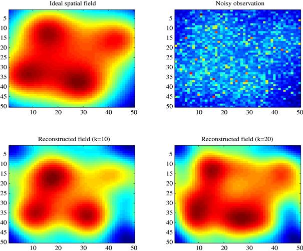
Figure 7.18 Example of field reconstruction in the presence of fading: ideal spatial field (top left); measured field (top right); field reconstructed with order ![]() (bottom left) and
(bottom left) and ![]() (bottom right) [75].
(bottom right) [75].
2.07.7 Minimum energy consensus
Although distributed algorithms to achieve consensus have received a lot of attention because of their capability of reaching optimal decisions without the need of a fusion center, the price paid for this simplicity is that consensus algorithms are inherently iterative. As a consequence the iterated exchange of data among the nodes might cause an excessive energy consumption. Hence, to make consensus algorithms really appealing in practical applications, it is necessary to minimize the energy consumption necessary to reach consensus. The network topology plays a fundamental role in determining the convergence rate [74]. As the network connectivity increases, so does the convergence rate. However, a highly connected network entails a high power consumption to guarantee reliable direct links between the nodes. On the other hand, if the network is minimally connected, with only neighbor nodes connected to each other, a low power is spent to maintain the few short range links, but, at the same time, a large convergence time is required. Since what really matters in a WSN is the overall energy spent to achieve consensus, in [76,77] it was considered the problem of finding the optimal network topology that minimizes the overall energy consumption, taking into account convergence time and transmit powers jointly. More specifically, in [77] it is proposed a method for optimizing the network topology and the power allocation across every link in order to minimize the energy necessary to achieve consensus. Two different types of networks are considered: a) deterministic topologies, where node positions are arbitrary, but known; b) random geometries, where the unknown node locations are modeled as random variables. We will now review the methodology used in both cases.
2.07.7.1 Optimization criterion
By considering only the power spent to enable wireless communications, the overall energy consumption to reach consensus can be written as the product between the sum of the power ![]() necessary to establish the communication links among the nodes and the number of iterations
necessary to establish the communication links among the nodes and the number of iterations ![]() necessary to achieve consensus. The exchange of information among the nodes is supposed to take place in the presence of a slotted system, with a medium access control (MAC) mechanism that prevents packet collisions. The number of iterations can be approximated as
necessary to achieve consensus. The exchange of information among the nodes is supposed to take place in the presence of a slotted system, with a medium access control (MAC) mechanism that prevents packet collisions. The number of iterations can be approximated as ![]() where
where ![]() denotes the duration of a time slot unit and
denotes the duration of a time slot unit and
![]()
is the convergence time defined as the time necessary for the slowest mode of the dynamical system (7.23) to be reduced by a factor ![]() . The total power spent by the network in each iteration is then
. The total power spent by the network in each iteration is then ![]() where the coefficient
where the coefficient ![]() denotes the power transmitted by node i to node j, while the binary coefficients
denotes the power transmitted by node i to node j, while the binary coefficients ![]() assess the presence (
assess the presence (![]() ) of a link between nodes i and j or not (
) of a link between nodes i and j or not (![]() ). Our goal is to minimize the energy consumption expressed by the following metric
). Our goal is to minimize the energy consumption expressed by the following metric
![]() (7.151)
(7.151)
where K incorporates all irrelevant constants, N is the number of sensors and ![]() is the Laplacian matrix depending on the vector
is the Laplacian matrix depending on the vector ![]() containing all the coefficients
containing all the coefficients ![]() . More specifically, we aim to find the set of active links, i.e., the non-zero coefficients
. More specifically, we aim to find the set of active links, i.e., the non-zero coefficients ![]() , and the powers
, and the powers ![]() that minimize the energy consumption (7.151), under the constraint of guaranteeing network connectivity, i.e., enforcing
that minimize the energy consumption (7.151), under the constraint of guaranteeing network connectivity, i.e., enforcing ![]() . The problem can be formulated as follows [77]:
. The problem can be formulated as follows [77]:
 (7.152)
where ![]() is an arbitrarily small positive constant used to ensure network connectivity and
is an arbitrarily small positive constant used to ensure network connectivity and ![]() is the vector with entries
is the vector with entries ![]() . Since the topology coefficients are binary variables, [P.0] is a combinatorial problem, with complexity increasing with the size N of the network as
. Since the topology coefficients are binary variables, [P.0] is a combinatorial problem, with complexity increasing with the size N of the network as ![]() . In [77] we have modified [P.0] in order to convert it into a convex problem, with negligible performance losses. A first simplification comes from observing that the coefficients
. In [77] we have modified [P.0] in order to convert it into a convex problem, with negligible performance losses. A first simplification comes from observing that the coefficients ![]() and
and ![]() are dependent of each other through the radio propagation model so that the set of unknowns can be reduced to the set of powers
are dependent of each other through the radio propagation model so that the set of unknowns can be reduced to the set of powers ![]() . More specifically, by assuming flat fading channel, we can assume that the power
. More specifically, by assuming flat fading channel, we can assume that the power ![]() received by node j when node i transmits is given by
received by node j when node i transmits is given by
![]() (7.153)
(7.153)
where ![]() is the distance between nodes i and
is the distance between nodes i and ![]() is the path loss exponent, and the parameter
is the path loss exponent, and the parameter ![]() corresponds to the so called Fraunhofer distance. We have included in the denominator the unitary term to avoid the unrealistic situation in which the received power could be greater than the transmitted one. Given the propagation model (7.153), the relation between the power coefficients
corresponds to the so called Fraunhofer distance. We have included in the denominator the unitary term to avoid the unrealistic situation in which the received power could be greater than the transmitted one. Given the propagation model (7.153), the relation between the power coefficients ![]() and the topology coefficients
and the topology coefficients ![]() is then
is then
 (7.154)
where ![]() is the minimum power needed at the receiver side to establish a communication. In [77] we have shown how to relax this relation in order to simplify the solution of the optimal topology control problem considering both the deterministic and random topology.
is the minimum power needed at the receiver side to establish a communication. In [77] we have shown how to relax this relation in order to simplify the solution of the optimal topology control problem considering both the deterministic and random topology.
2.07.7.2 Optimal topology and power allocation for arbitrary networks
In the case where the distances between the nodes are known, to find the optimal solution of problem [P.0] involves a combinatorial strategy that makes the problem numerically very hard to solve. In [77], we have relaxed problem [P.0] so that, instead of requiring ![]() to be binary, we assume
to be binary, we assume ![]() to be a real variable belonging to the interval
to be a real variable belonging to the interval ![]() . This relaxation is the first step to transform the previous problem into a convex problem. More specifically, we have introduced the following relationship between the coefficients
. This relaxation is the first step to transform the previous problem into a convex problem. More specifically, we have introduced the following relationship between the coefficients ![]() and the distances
and the distances ![]() :
:
![]() (7.155)
(7.155)
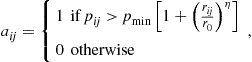
where ![]() is a positive coefficient and
is a positive coefficient and ![]() is the coverage radius, which depends on the transmit power. According to (7.155),
is the coverage radius, which depends on the transmit power. According to (7.155), ![]() is close to one when node j is within the coverage radius of node i, i.e.,
is close to one when node j is within the coverage radius of node i, i.e., ![]() , whereas
, whereas ![]() is close to zero, when
is close to zero, when ![]() . The switching from zero to one can be made steeper by increasing the value of
. The switching from zero to one can be made steeper by increasing the value of ![]() . In [77] we have found the coefficients
. In [77] we have found the coefficients ![]() as a function of
as a function of ![]()
 (7.156)
with ![]() . Consequently, we can reduce the set of variables to the only power vector
. Consequently, we can reduce the set of variables to the only power vector ![]() and problem [P.0] can be relaxed into the following problem:
and problem [P.0] can be relaxed into the following problem:
 (7.157)
The first important result proved in [77] is that the problem [P.1] is a convex-concave fractional problem if ![]() , so that we can use one of the methods that solve quasi-convex optimization problems, see e.g., [78,79]. In [77] we have used the nonlinear parametric formulation proposed in [79]. Hence we have further converted the convex-concave fractional problem [P.1] into the following equivalent parametric problem in terms of vector
, so that we can use one of the methods that solve quasi-convex optimization problems, see e.g., [78,79]. In [77] we have used the nonlinear parametric formulation proposed in [79]. Hence we have further converted the convex-concave fractional problem [P.1] into the following equivalent parametric problem in terms of vector ![]() , i.e.,
, i.e.,
 (7.158)
where ![]() and
and ![]() controls the trade-off between total transmit power and convergence time.
controls the trade-off between total transmit power and convergence time.
The optimization problem [P.2] is a convex parametric problem [77] and an optimal solution can be found via efficient numerical tools. Furthermore, using Dinkelbach’s algorithm [79], we are also able to find the optimal parameter ![]() in [P.2].
in [P.2].
2.07.7.3 Numerical examples
Since our optimization procedure is based on a relaxation technique, we have evaluated the impact of the relaxation on the final topology and performance.
More specifically, the topology coefficients ![]() obtained by solving [P.2] are real variables belonging to the interval
obtained by solving [P.2] are real variables belonging to the interval ![]() , so that, to obtain the network topology, it is necessary a quantization step to convert them into binary values, 1 or 0, by comparing each
, so that, to obtain the network topology, it is necessary a quantization step to convert them into binary values, 1 or 0, by comparing each ![]() with a threshold
with a threshold ![]() . It has been shown that the loss in terms of optimal energy due to the relaxation of the original problem is negligible. To evaluate the impact of thresholding operation, in Figure 7.19 we show the topologies obtained by solving problem [P.2], for a network composed of
. It has been shown that the loss in terms of optimal energy due to the relaxation of the original problem is negligible. To evaluate the impact of thresholding operation, in Figure 7.19 we show the topologies obtained by solving problem [P.2], for a network composed of ![]() nodes, using different values of
nodes, using different values of ![]() and assuming
and assuming ![]() . Comparing the four cases reported in Figure 7.19, we can note that for a large range of values of
. Comparing the four cases reported in Figure 7.19, we can note that for a large range of values of ![]() , the final topology is practically the same, while only for very low values of the threshold (i.e., case (d)), we can observe a sensitive change of topology. This means that the relaxation method is robust against the choice of the final threshold.
, the final topology is practically the same, while only for very low values of the threshold (i.e., case (d)), we can observe a sensitive change of topology. This means that the relaxation method is robust against the choice of the final threshold.

The previous results pertain to a specific realization of the node locations. To provide results of more general validity, in Figure 7.20, we report the average value of (a) the energy (![]() ) (b)
) (b) ![]() , and (c) fraction of active links
, and (c) fraction of active links ![]() , as a function of the path loss exponent
, as a function of the path loss exponent ![]() , setting
, setting ![]() . From Figure 7.20, we observe that when the attenuation is high (i.e.,
. From Figure 7.20, we observe that when the attenuation is high (i.e., ![]() is large), reducing the number of links (making the topology sparser) is more important than reducing convergence time. Conversely, when the attenuation is low (i.e.,
is large), reducing the number of links (making the topology sparser) is more important than reducing convergence time. Conversely, when the attenuation is low (i.e., ![]() is small), increasing network connectivity is more important than reducing power consumption.
is small), increasing network connectivity is more important than reducing power consumption.
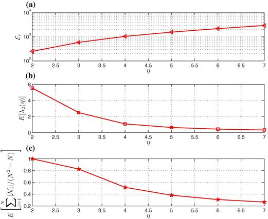
2.07.7.4 Minimization of the energy consumption over random geometric graphs
Let us consider now the problem of minimizing the energy consumption for a sensor network modeled as a random geometric graph. We will use the symbol ![]() to indicate an RGG composed of N points, with coverage radius r.
to indicate an RGG composed of N points, with coverage radius r.
In [74], it has been shown that the degree of an RGG ![]() of points uniformly distributed over a two-dimensional unit torus7 is equal to
of points uniformly distributed over a two-dimensional unit torus7 is equal to
![]() (7.159)
(7.159)
with high probability, i.e., with probability ![]() , if the radius behaves as
, if the radius behaves as ![]() in (7.2). This implies that if the coverage radius is chosen so as to guarantee connectivity with high probability, an RGG tends to behave, asymptotically, as a regular graph. In order to calculate the convergence rate we have to derive the second eigenvalue of the Laplacian,
in (7.2). This implies that if the coverage radius is chosen so as to guarantee connectivity with high probability, an RGG tends to behave, asymptotically, as a regular graph. In order to calculate the convergence rate we have to derive the second eigenvalue of the Laplacian, ![]() , where
, where ![]() is the degree matrix and
is the degree matrix and ![]() is the adjacency matrix. From (7.159),
is the adjacency matrix. From (7.159), ![]() , so that we only need to calculate the second largest eigenvalue of
, so that we only need to calculate the second largest eigenvalue of ![]() . In Appendix A.2, we study the asymptotic behavior of the spectrum of
. In Appendix A.2, we study the asymptotic behavior of the spectrum of ![]() and the result is that the second largest eigenvalue of
and the result is that the second largest eigenvalue of ![]() tends asymptotically to
tends asymptotically to
![]() (7.160)
(7.160)
where r is the coverage radius of each node.
2.07.7.4.1 An analytic approach for minimizing the energy consumption
In [77] we studied the energy minimization problem for RGG’s, exploiting the previous analytic expressions. In the random topology case, since the distances are unknown, we cannot optimize the power associated with each link. However, we can seek the common transmit power that minimizes energy consumption. Thus, in the random setting we assume a broadcast communication model, where each node broadcasts the value to be shared with its neighbors. In the lack of any information about distances among the nodes, we assume that each node uses the same transmit power. In this case, the network topology can be modeled as a random graph model. In [80,81] it has been shown that the dynamical system ![]() converges to consensus almost surely, i.e.,
converges to consensus almost surely, i.e., ![]() assuming that each node has a coverage radius so that the network is asymptotically connected with probability one. Then the rate of convergence to consensus is given [80,81] by
assuming that each node has a coverage radius so that the network is asymptotically connected with probability one. Then the rate of convergence to consensus is given [80,81] by ![]() . In [77] we proved that the convergence rate can be approximated as
. In [77] we proved that the convergence rate can be approximated as
![]() (7.161)
(7.161)
so that the energy spent to achieve consensus can now be expressed as
![]() (7.162)
(7.162)
This is the performance metric we wish to minimize in the random scenario, with respect to the single unknown p.
In particular, using the asymptotic expression (7.160) for the algebraic connectivity, we can introduce the following metric
![]() (7.163)
(7.163)
that is a convex function of r, for ![]() , where
, where ![]() , behaves as in (7.2) to ensure connectivity.Numerical examples. In Figure 7.21, we compare the value of
, behaves as in (7.2) to ensure connectivity.Numerical examples. In Figure 7.21, we compare the value of ![]() obtained by our theoretical approach and by simulation, for various values of the path loss exponent
obtained by our theoretical approach and by simulation, for various values of the path loss exponent ![]() . The results are averaged over 100 independent realizations of random geometric graphs composed of
. The results are averaged over 100 independent realizations of random geometric graphs composed of ![]() nodes. For each
nodes. For each ![]() , we indicate the pair of radius and energy providing minimum energy consumption by a circle (simulation) or a star (theory). It can be noted that the theoretical derivations provide a very good prediction of the performance achieved by simulation and, for each
, we indicate the pair of radius and energy providing minimum energy consumption by a circle (simulation) or a star (theory). It can be noted that the theoretical derivations provide a very good prediction of the performance achieved by simulation and, for each ![]() , there is a coverage radius value that minimizes energy consumption.
, there is a coverage radius value that minimizes energy consumption.
2.07.8 Matching communication network topology to statistical dependency graph
In Section 2.07.2.2, we saw that the topology of a sensor network observing a random field should depend on the structure of the graph describing the observed field. In this section, we recall a method proposed in [82,83] to design the topology of a wireless sensor network observing a Markov random field in order to match the structure of the dependency graph of the observed field, under constraints on the power used to ensure the sensor network connectivity. As in [82,83], our main task is to recover the sparsity of the dependency graph and to replicate it at the sensor network level, under the constraint of limiting the transmit power necessary to establish the link among the nodes. Also in this case, searching for an optimal topology is a combinatorial problem. To avoid the computational burden of solving the combinatorial problem, we propose an ad hoc relaxation technique that allows us to achieve the solution through efficient algorithms based on difference of convex problems.
Let us assume to have a network composed of N nodes, each one observing a spatial sample of a Gaussian Markov Random Field. We denote by ![]() the vector of the observations collected by the N nodes and we assume that
the vector of the observations collected by the N nodes and we assume that ![]() has zero mean and covariance matrix
has zero mean and covariance matrix ![]() . The statistical dependency among the random variables
. The statistical dependency among the random variables ![]() is well captured by the structure of the Markov graph whose vertices correspond to the random variables and whose links denote statistical dependencies among the variables. As discussed in 2.07.2.2 the main feature of a Markov graph is that it is sparse and there is no link between two nodes if and only if their observations are statistically independent. Moreover, if the random vector
is well captured by the structure of the Markov graph whose vertices correspond to the random variables and whose links denote statistical dependencies among the variables. As discussed in 2.07.2.2 the main feature of a Markov graph is that it is sparse and there is no link between two nodes if and only if their observations are statistically independent. Moreover, if the random vector ![]() is also Gaussian, with covariance matrix
is also Gaussian, with covariance matrix ![]() , the sparsity of the Markov graph is completely specified by the sparsity of the precision matrix, which is the inverse of the covariance matrix, i.e.,
, the sparsity of the Markov graph is completely specified by the sparsity of the precision matrix, which is the inverse of the covariance matrix, i.e., ![]() . On the other hand, the topology of the WSN can also be described by a graph, having adjacency matrix
. On the other hand, the topology of the WSN can also be described by a graph, having adjacency matrix ![]() such that
such that ![]() only if there is a physical link between nodes i and j. We use a simple propagation model such that there is a link between node i and j if the power received by node j exceeds a minimum power
only if there is a physical link between nodes i and j. We use a simple propagation model such that there is a link between node i and j if the power received by node j exceeds a minimum power ![]() . The received power depends on the power
. The received power depends on the power ![]() used by node i to transmit to node j and on the distance
used by node i to transmit to node j and on the distance ![]() between nodes i and j through the equation
between nodes i and j through the equation
![]() (7.164)
(7.164)
where ![]() is the path loss exponent.
is the path loss exponent.
As proposed in [82,83], our goal is to design the topology of the WSN, and hence its adjacency matrix ![]() , in order to match as well as possible the topology of the dependency graph, compatibly with the power expenditure necessary to establish each link in the network. Without any power constraint, we would choose
, in order to match as well as possible the topology of the dependency graph, compatibly with the power expenditure necessary to establish each link in the network. Without any power constraint, we would choose ![]() to be equal to
to be equal to ![]() , so as to reproduce the same sparsity of the dependency graph. Adding the power constraints, we will end up, in general, with a matrix
, so as to reproduce the same sparsity of the dependency graph. Adding the power constraints, we will end up, in general, with a matrix ![]() different from
different from ![]() . We measure the difference between the two matrices
. We measure the difference between the two matrices ![]() and
and ![]() using the so called Burg divergence, defined as
using the so called Burg divergence, defined as
![]() (7.165)
(7.165)
Even though the Burg divergence does not respect all the prerequisites to be a distance, it holds true that ![]() , if and only if
, if and only if ![]() , otherwise, the divergence is strictly positive. If the matrices
, otherwise, the divergence is strictly positive. If the matrices ![]() and
and ![]() are definite positive, the expression in (7.165) coincides with the Kullback-Leibler divergence between the probability density function (pdf) of two Gaussian random vectors having zero mean and precision matrices
are definite positive, the expression in (7.165) coincides with the Kullback-Leibler divergence between the probability density function (pdf) of two Gaussian random vectors having zero mean and precision matrices ![]() and
and ![]() or, equivalently, covariance matrices
or, equivalently, covariance matrices ![]() and
and ![]() .
.
2.07.8.1 Encouraging sparsity by preserving total transmit power
One of the most important tasks in wireless sensor networks is to minimize the energy consumption for reliable data transmission. This need can be accommodated by formulating the search for a sparse topology incorporating a penalization for the presence of links among distant nodes. The first strategy we propose is named Sparsity with Minimum Power (SMP) consumption. We consider both cases where the covariance matrix is perfectly known or estimated from the collected data.
Let us consider a wireless sensor network whose communication graph is a geometric graph, where each node communicates only with the nodes lying within its coverage area of radius r. We assume, initially, that the covariance matrix ![]() of the GMRF is perfectly known. Our goal is to find the optimal adjacency matrix
of the GMRF is perfectly known. Our goal is to find the optimal adjacency matrix ![]() that minimizes the divergence
that minimizes the divergence ![]() given in (7.165), under the constraint of limiting the transmit power necessary to maintain the links among the nodes of the WSN. This constraint can be incorporated in our optimization problem by introducing a penalty term given by the sum of the transmit powers over all active links, i.e.,
given in (7.165), under the constraint of limiting the transmit power necessary to maintain the links among the nodes of the WSN. This constraint can be incorporated in our optimization problem by introducing a penalty term given by the sum of the transmit powers over all active links, i.e.,
 (7.166)
where ![]() denotes the power used by node i to transmit to node j and
denotes the power used by node i to transmit to node j and
 (7.167)
assuming that ![]() is different from zero only if the power
is different from zero only if the power ![]() received by node j when node i transmits, as given in (7.164), exceeds a suitable minimum level
received by node j when node i transmits, as given in (7.164), exceeds a suitable minimum level ![]() , i.e., if
, i.e., if
![]() (7.168)
(7.168)
The optimization problem can then be formulated as
![]() (7.169)
(7.169)
where ![]() is the cone of definite positive symmetric
is the cone of definite positive symmetric ![]() -dimensional matrices, while
-dimensional matrices, while ![]() is the penalty coefficient introduced to control sparsity. In fact, increasing the penalty coefficient, we assign a higher weight to power consumption so that sparse structures are more likely to occur.
is the penalty coefficient introduced to control sparsity. In fact, increasing the penalty coefficient, we assign a higher weight to power consumption so that sparse structures are more likely to occur.
Problem (7.169) is indeed quite hard to solve as the penalty function is a nonconvex discrete function. Optimization problems with a convex penalty have been largely considered in several signal processing applications, for example in compressed sensing [84] where these problems are often formulated as a penalized least-square problem in which sparsity is usually induced by adding a ![]() -norm penalty on the coefficients, as in Lasso algorithm [47].
-norm penalty on the coefficients, as in Lasso algorithm [47].
Indeed, non-convex penalty functions such as ![]() -norm, with
-norm, with ![]() , are even more effective to recover sparsity than
, are even more effective to recover sparsity than ![]() -norm. Actually, using the so called
-norm. Actually, using the so called ![]() norm would be even more effective to measure sparsity, even though the
norm would be even more effective to measure sparsity, even though the ![]() norm does not respect all requisites to be a norm.8 Here we adopt the so called Zhang penalty function analyzed in [85], i.e.,
norm does not respect all requisites to be a norm.8 Here we adopt the so called Zhang penalty function analyzed in [85], i.e.,
 (7.170)
where ![]() is an infinitesimal positive constant. Hence, by assuming
is an infinitesimal positive constant. Hence, by assuming ![]() , the second term in (7.169) can be written as
, the second term in (7.169) can be written as
 (7.171)
where ![]() is a
is a ![]() dimensional symmetric matrix with entries
dimensional symmetric matrix with entries ![]() ,
, ![]() , while the matrix mapping
, while the matrix mapping ![]() is defined applying the elementwise mapping
is defined applying the elementwise mapping ![]() given in (7.170). The combinatorial problem in (7.169) can then be reformulated as
given in (7.170). The combinatorial problem in (7.169) can then be reformulated as
![]() (7.172)
(7.172)
Unfortunately the second term in (7.172), is not convex so that the problem we have to solve is a nonconvex, nonsmooth optimization problem. Nevertheless, in [82,83] we reformulated this problem as a difference of convex (DC) problem. Before proceeding, we simply illustrate how to extend our approach to the case where the covariance matrix of the observed vector is not known but estimated from the data. In such a case, the matrix ![]() in (7.172) is substituted by the estimated matrix
in (7.172) is substituted by the estimated matrix ![]() , whose entry
, whose entry ![]() is
is
 (7.173)
where ![]() is the observation collected by node i, at time k, with
is the observation collected by node i, at time k, with ![]() . The practical, relevant, difference is that while the true precision matrix
. The practical, relevant, difference is that while the true precision matrix ![]() is sparse by hypothesis, the inverse of
is sparse by hypothesis, the inverse of ![]() in general is not sparse. Also in this case, encouraging sparsity in estimating the inverse of the covariance matrix can be beneficial to improve the quality of the estimation itself.9
in general is not sparse. Also in this case, encouraging sparsity in estimating the inverse of the covariance matrix can be beneficial to improve the quality of the estimation itself.9
The problem (7.172) can be reformulated as a Difference of Convex (DC) functions problem [86], by decomposing the function ![]() as the difference of two convex functions
as the difference of two convex functions ![]() with
with ![]() and
and
 (7.174)
Hence the optimization problem in (7.172) can be rewritten as
![]() (7.175)
(7.175)
To solve this problem, we have used an iterative procedure, known as DC algorithm (DCA), based on the duality of DC programming. The usefulness of using DCA is that its convergence has been proved in [86] and it is simple to implement, as it iteratively solves a convex optimization problem. We refer the reader to [82,83] for further analytical details.
2.07.8.2 Sparsification and estimation of the precision matrix
In this section we illustrate an alternative sparsification strategy that improves the estimate of the precision matrix with respect to the SMP strategy. In this alternative formulation, the penalty term is the sum of the absolute values of the entries of ![]() , weighted with the corresponding per-link transmit power consumption. In this way, although the power consumption should not be lower than the SMP method, we expect a sparse topology with a more accurate estimate of the precision matrix. We call this strategy Sparse Estimation Strategy (SES). The new problem is formulated as follows
, weighted with the corresponding per-link transmit power consumption. In this way, although the power consumption should not be lower than the SMP method, we expect a sparse topology with a more accurate estimate of the precision matrix. We call this strategy Sparse Estimation Strategy (SES). The new problem is formulated as follows
![]() (7.176)
(7.176)
and it can be converted into a convex definite positive problem. In particular, splitting the matrix ![]() into the difference of two nonnegative matrices representing its positive and negative part, i.e.,
into the difference of two nonnegative matrices representing its positive and negative part, i.e., ![]() , we can rewrite (7.176) as
, we can rewrite (7.176) as
 (7.177)
![]()
This problem can be solved using standard numerical tools or by applying a projected gradient algorithm [87].
2.07.8.3 Numerical results
In this section we report some simulation results considering a sensors network composed of ![]() nodes, uniformly deployed over a unit area square and observing correlated data from a GMRF. We adopt the Markov model proposed in [8], where the correlation between neighboring nodes is a decreasing function of their distance and the entries of the covariance matrix can be derived in closed form. In [82,83] we have shown that even though the problem is not convex, the numerical results seem to indicate that the method always converges to the same value of the precision matrix entries, irrespective of the initializations. In Figure 7.22 we report the final optimal network topology referring to the case of a matrix estimated from the data. In particular, the top left plot of Figure 7.22 shows the true dependency graph and all other plots depict the network topologies obtained using the proposed SMP algorithm, with different penalty coefficients. More specifically, the network topologies shown in Figure 7.22 are obtained by thresholding the values of the matrix
nodes, uniformly deployed over a unit area square and observing correlated data from a GMRF. We adopt the Markov model proposed in [8], where the correlation between neighboring nodes is a decreasing function of their distance and the entries of the covariance matrix can be derived in closed form. In [82,83] we have shown that even though the problem is not convex, the numerical results seem to indicate that the method always converges to the same value of the precision matrix entries, irrespective of the initializations. In Figure 7.22 we report the final optimal network topology referring to the case of a matrix estimated from the data. In particular, the top left plot of Figure 7.22 shows the true dependency graph and all other plots depict the network topologies obtained using the proposed SMP algorithm, with different penalty coefficients. More specifically, the network topologies shown in Figure 7.22 are obtained by thresholding the values of the matrix ![]() obtained through our SMP algorithm, i.e., the coefficients of matrix
obtained through our SMP algorithm, i.e., the coefficients of matrix ![]() are set to zero if
are set to zero if ![]() . In the top right plot of Figure 7.22, it can be noted that the precision matrix achieved with a null penalty can be quite dense because of estimation errors. Nevertheless, it is interesting to observe that, as the penalty coefficient increases, the proposed method is not only able to recover the desired topology, but also to correct most of the errors due to estimation. We can say that the introduction of the penalty induces a robustness against estimation errors. Let us now compare the SMP method with the SES strategy, by considering a data estimated covariance matrix in the divergence term and averaging the simulation results over 100 independent realizations of the nodes deployment. Let us now evaluate the mismatch between the network topology and the dependency graph, as a function of the penalty coefficient, obtained using the two proposed strategies. We assess the mismatch by counting the number of links appearing in the network topology, which do not appear in the dependency graph. To this end, Figure 7.23 shows the fraction of incorrect links
. In the top right plot of Figure 7.22, it can be noted that the precision matrix achieved with a null penalty can be quite dense because of estimation errors. Nevertheless, it is interesting to observe that, as the penalty coefficient increases, the proposed method is not only able to recover the desired topology, but also to correct most of the errors due to estimation. We can say that the introduction of the penalty induces a robustness against estimation errors. Let us now compare the SMP method with the SES strategy, by considering a data estimated covariance matrix in the divergence term and averaging the simulation results over 100 independent realizations of the nodes deployment. Let us now evaluate the mismatch between the network topology and the dependency graph, as a function of the penalty coefficient, obtained using the two proposed strategies. We assess the mismatch by counting the number of links appearing in the network topology, which do not appear in the dependency graph. To this end, Figure 7.23 shows the fraction of incorrect links ![]() , normalized to the total number of links
, normalized to the total number of links ![]() , versus
, versus ![]() . More specifically, considering the true and optimal precision matrices (
. More specifically, considering the true and optimal precision matrices (![]() and
and ![]() respectively), we can define
respectively), we can define ![]() where
where ![]() if
if ![]() and
and ![]() are not equal, assuming
are not equal, assuming ![]() if
if ![]() and zero otherwise. From Figure 7.23, we can deduce that SES provides more correct links than SMP, as it achieves lower values of
and zero otherwise. From Figure 7.23, we can deduce that SES provides more correct links than SMP, as it achieves lower values of ![]() .
.
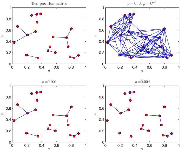
2.07.9 Conclusions and further developments
In this article we have provided a general framework to show how an efficient design of a wireless sensor network requires a joint combination of in-network processing and communication. In particular, we have shown that inferring the structure of the graph describing the statistical dependencies among the observed data can provide important information on how to build the sensor network topology and how to design the flow of information through the network. We have illustrated several possible network architectures where the global decisions, either estimation or hypothesis testing, are taken by a central node or in a totally decentralized way. In particular, various forms of consensus have been shown to be instrumental to achieve globally optimal performance through local interactions only. Consensus algorithms have then been generalized to more sophisticated signal processing techniques able to provide a cartography of the observed field. In a decentralized framework, the network topology plays an important role in terms of convergence time as well as structure of the final consensus value. Considering that most sensor networks exchange information through a wireless channel, we have addressed the problem of finding the network topology that minimizes the energy consumption required to reach consensus. Finally, we have showed how to match the network topology to the Markov graph describing the observed variables, under constraints imposed by the power consumption necessary to establish direct links among the sensor nodes.
Even though the field of distributed detection and estimation has accumulated an enormous amount of research works, there are still many open problems, both in the theoretical as well as in the application sides. In the following we make a short list of possible topics of future interest.
1. The general multi-terminal source/channel coding problem is still an open issue. The conventional paradigm established by the source/channel coding separation theorem does not hold for the multi-terminal case. This means that source coding should be studied jointly with channel coding.
2. Distributed decision establishes a strict link between statistical signal processing and graph theory. In particular, the network topology plays a fundamental role in the design of an efficient sensor network. In this chapter, we have shown some simple techniques aimed to matching the network topology to the statistical dependency graph of the observed variables, but significant improvements may be expected from cross-fertilization of methods from graph theory and statistical signal processing.
3. The design of fully decentralized detection algorithms has already received important contributions. Nevertheless, there are many open issues concerning the refinements of the local decision thresholds as a function of both local observations and the decisions taken from neighbors. In a more general setting, social learning is expected to play an important role in future sensor networks.
4. An efficient design of wireless sensor networks requires a strict relation between radio resource allocation and decision aspects, under physical constraints dictated by energy limitations or channel noise and interference. Some preliminary results have been achieved in the many-to-one setting, but the general many-to-many case needs to be thoroughly studied.
5. The application of wireless sensor networks to new fields may be easily expected. The important remark is that, to improve the efficiency of the network at various levels, it is necessary to take the application needs strictly into account in the network design. In other words, a cross-layer design incorporating all layers from the application down to the physical layer is especially required in sensor networks. Clearly, handling the complexity of the network will require some sort of layering, but this layering will not necessarily be the same as in telecommunication networks, because the requirements and constraints in the two fields are completely different.
Appendix A
In this appendix we briefly review some important notations and basic concepts of graph theory that have been adopted in the previous sections (for a more detailed introduction to this field see [13]).
A.1 Algebraic graph theory
Given N nodes let us define a directed graph or digraph![]() as a set of nodes
as a set of nodes ![]() and a set of edges or links
and a set of edges or links ![]() where the links
where the links ![]() connect the ordered pair of nodes
connect the ordered pair of nodes ![]() , with the convention that the information flows from
, with the convention that the information flows from ![]() to
to ![]() . In the case where a positive weight
. In the case where a positive weight ![]() is associated to each edge, the digraph is called weighted. Let us assume that there are no loops, i.e.,
is associated to each edge, the digraph is called weighted. Let us assume that there are no loops, i.e., ![]() .
.
The graph is called undirected if ![]() . The in-degree and out-degree of node
. The in-degree and out-degree of node ![]() are, respectively, defined as
are, respectively, defined as ![]() and
and ![]() . In the case of undirected graphs
. In the case of undirected graphs ![]() . Let
. Let ![]() denote the set of neighbors of node i, so that
denote the set of neighbors of node i, so that ![]() .
.
The node ![]() of a digraph is said to be balanced if and only if its in-degree and out-degree coincide, while a digraph is called balanced if and only if all its nodes are balanced.
of a digraph is said to be balanced if and only if its in-degree and out-degree coincide, while a digraph is called balanced if and only if all its nodes are balanced.
We recall now the basic properties of the matrices associated to a digraph, as they play a fundamental role in the study of the connectivity of the network associated to the graph. Given a digraph ![]() , we introduce the following matrices associated with
, we introduce the following matrices associated with ![]() : (1) The
: (1) The ![]() adjacency matrix
adjacency matrix ![]() whose entries
whose entries ![]() are equal to the weight associated to the edge
are equal to the weight associated to the edge ![]() , or equal to zero, otherwise; (2) the degree matrix
, or equal to zero, otherwise; (2) the degree matrix ![]() which is the diagonal matrix whose diagonal entries are
which is the diagonal matrix whose diagonal entries are ![]() ; (3) the weighted Laplacian matrix
; (3) the weighted Laplacian matrix ![]() , defined as
, defined as ![]() whose entries are
whose entries are
 (7.178)
According to this definition ![]() has the following properties: (a) its diagonal elements are positive; (b) it has zero row sum; (c) it is a diagonally row dominant matrix. It can be easily verified that
has the following properties: (a) its diagonal elements are positive; (b) it has zero row sum; (c) it is a diagonally row dominant matrix. It can be easily verified that ![]() ,10 i.e., zero is an eigenvalue of
,10 i.e., zero is an eigenvalue of ![]() corresponding to a right eigenvector
corresponding to a right eigenvector ![]() in the
in the ![]() , and all the other eigenvalues have positive real parts. Furthermore a digraph is balanced if and only if
, and all the other eigenvalues have positive real parts. Furthermore a digraph is balanced if and only if ![]() is also a left eigenvector of
is also a left eigenvector of ![]() associated with the zero eigenvalue or
associated with the zero eigenvalue or ![]() . Note that for undirected graph the Laplacian matrix is a symmetric and then balanced matrix with non negative real eigenvalues.
. Note that for undirected graph the Laplacian matrix is a symmetric and then balanced matrix with non negative real eigenvalues.
The algebraic multiplicity of the zero eigenvalue of ![]() is equal to the number of connected components contained in
is equal to the number of connected components contained in ![]() . For undirected graphs
. For undirected graphs ![]() is connected if and only if the algebraic multiplicity of the zero eigenvalue is 1, or, equivalently,
is connected if and only if the algebraic multiplicity of the zero eigenvalue is 1, or, equivalently, ![]() if and only if
if and only if ![]() is connected. Hence, if an undirected graph is connected, the eigenvector associated with the zero eigenvalue is
is connected. Hence, if an undirected graph is connected, the eigenvector associated with the zero eigenvalue is ![]() , and the second smallest eigenvalue of
, and the second smallest eigenvalue of ![]() , denoted as
, denoted as ![]() and called algebraic connectivity [22] of
and called algebraic connectivity [22] of ![]() , is strictly positive.
, is strictly positive.
A.1.1 Forms of connectivity for digraphs
Before to introduce several forms of graph connectivity [17] we have to define some useful concepts. A strong path of a digraph ![]() is a sequence of distinct nodes
is a sequence of distinct nodes ![]() such that
such that ![]() , for
, for ![]() . If
. If ![]() , the path is said to be closed. A weak path is a sequence of distinct nodes
, the path is said to be closed. A weak path is a sequence of distinct nodes ![]() such that either
such that either ![]() or
or ![]() , for
, for ![]() . A closed strong path is said a strong cycle. A digraph with N nodes is a directed tree if it has
. A closed strong path is said a strong cycle. A digraph with N nodes is a directed tree if it has ![]() edges and there exists a node, called the root node, which can reach all the other nodes through an unique strong path. As a consequence a directed tree contains no cycles and every node, except the root, has one and only one incoming edge. A digraph is a forest if it consists of one or more directed trees. A subgraph
edges and there exists a node, called the root node, which can reach all the other nodes through an unique strong path. As a consequence a directed tree contains no cycles and every node, except the root, has one and only one incoming edge. A digraph is a forest if it consists of one or more directed trees. A subgraph ![]() of a digraph
of a digraph ![]() , with
, with ![]() and
and ![]() , is a directed spanning tree (or a spanning forest) if it is a directed tree (or a directed forest) and it has the same node set as
, is a directed spanning tree (or a spanning forest) if it is a directed tree (or a directed forest) and it has the same node set as ![]() .
.
According to this definition we can define many forms of connectivity [17]: (a) a digraph is strongly connected (SC) if any ordered pair of distinct nodes can be joined by a strong path; (b) a digraph is quasi strongly connected (QSC) if, for every ordered pair of nodes ![]() and
and ![]() , there exists a node r that can reach both
, there exists a node r that can reach both ![]() and
and ![]() via a strong path; (c) a digraph is weakly connected (WC) if any ordered pair of distinct nodes can be joined by a weak path; (d) a digraph is disconnected if it is not weakly connected. Note that for undirected graphs, the above notions of connectivity are equivalent. Moreover, it is easy to check that the quasi strong connectivity of a digraph is equivalent to the existence of a directed spanning tree in the graph.
via a strong path; (c) a digraph is weakly connected (WC) if any ordered pair of distinct nodes can be joined by a weak path; (d) a digraph is disconnected if it is not weakly connected. Note that for undirected graphs, the above notions of connectivity are equivalent. Moreover, it is easy to check that the quasi strong connectivity of a digraph is equivalent to the existence of a directed spanning tree in the graph.
A.1.2 Connectivity study from the condensation digraph
When a digraph ![]() is WC, it may still contain strongly connected subgraphs. A maximal subgraph of
is WC, it may still contain strongly connected subgraphs. A maximal subgraph of ![]() , which is also SC, is called a strongly connected component (SCC) of
, which is also SC, is called a strongly connected component (SCC) of ![]() [17,88]. Any digraph
[17,88]. Any digraph ![]() can be partitioned into SCCs, let us say
can be partitioned into SCCs, let us say ![]() where
where ![]() and
and ![]() for
for ![]() . The connectivity properties of a digraph may be better studied by referring to its corresponding condensation digraph. We may reduce the original digraph
. The connectivity properties of a digraph may be better studied by referring to its corresponding condensation digraph. We may reduce the original digraph ![]() to the condensation digraph
to the condensation digraph ![]() by associating the node set
by associating the node set ![]() of each SCC
of each SCC ![]() of
of ![]() to a single distinct node
to a single distinct node ![]() of
of ![]() and introducing an edge in
and introducing an edge in ![]() from
from ![]() to
to ![]() , if and only if there exists some edges from the SCC
, if and only if there exists some edges from the SCC ![]() and the SCC
and the SCC ![]() of the original graph. An SCC that is reduced to the root of a directed spanning tree of the condensation digraph is called the root SCC (RSCC). Looking at the condensation graph, we may identify the following topologies of the original graph: (1)
of the original graph. An SCC that is reduced to the root of a directed spanning tree of the condensation digraph is called the root SCC (RSCC). Looking at the condensation graph, we may identify the following topologies of the original graph: (1) ![]() is SC if and only if
is SC if and only if ![]() is composed by a single node; (2)
is composed by a single node; (2) ![]() is QSC if and only if
is QSC if and only if ![]() contains a directed spanning tree; (3) if
contains a directed spanning tree; (3) if ![]() is WC, then
is WC, then ![]() contains either a spanning tree or a (weakly) connected forest.
contains either a spanning tree or a (weakly) connected forest.
The multiplicity of the zero eigenvalue of ![]() is equal to the minimum number of directed trees contained in a directed spanning forest of
is equal to the minimum number of directed trees contained in a directed spanning forest of ![]() . Moreover, the zero eigenvalue of
. Moreover, the zero eigenvalue of ![]() is simple if and only if
is simple if and only if ![]() contains a spanning directed tree or, equivalently,
contains a spanning directed tree or, equivalently, ![]() is QSC. If
is QSC. If ![]() is SC then
is SC then ![]() has a simple zero eigenvalue and positive left-eigenvector associated to the zero eigenvalue. If
has a simple zero eigenvalue and positive left-eigenvector associated to the zero eigenvalue. If ![]() is QSC [17] with
is QSC [17] with ![]() strongly connected components
strongly connected components ![]() with
with ![]() for
for ![]() and
and ![]() , numbered w.l.o.g. so that
, numbered w.l.o.g. so that ![]() coincides with the root SCC of
coincides with the root SCC of ![]() , then the left-eigenvector
, then the left-eigenvector ![]() of
of ![]() associated to the zero eigenvalue has entries
associated to the zero eigenvalue has entries ![]() iff
iff ![]() and zero otherwise. If
and zero otherwise. If ![]() is balanced then
is balanced then ![]() where
where ![]() .
.
As a numerical example, in Figure 7.24 we report three network topologies: (a) a SC digraph; (b) a QSC digraph with three SCCs; (c) a WC digraph with a two-trees forest. We have also depicted for each digraph its decomposition into SCCs corresponding to the nodes of the associated condensation digraph; RSCC denotes the root SCC. For each network topology, we have also reported the dynamical evolution of the consensus algorithm in (7.23) versus time. It can be observed that the dynamical system in Figure 7.24a achieves a global consensus since the underlying digraph is SC. For the QSC digraph in Figure 7.24b, instead, there is a set of nodes in the RSCC component that is able to reach all other nodes so that the dynamical system can achieve a global consensus. Finally, in Figure 7.24c, the system cannot achieve a global consensus since there is no node that can reach all the others. Although we can observe two disjoint clusters corresponding to the two RSCC components, the nodes of the SCC component (middle lines) are affected by the consensus in the two RSCC components but are not able to influence them.
A.2 RGG adjacency matrix
A random graph is obtained by distributing N points randomly over the d-dimensional space ![]() and connecting the nodes according to a given rule. The graph topology is captured by the adjacency matrix
and connecting the nodes according to a given rule. The graph topology is captured by the adjacency matrix ![]() which, in this case, is a random matrix. An important class of random matrices, is the so called Euclidean Random Matrix (ERM) class, introduced in [89]. Given a set of N points located at positions
which, in this case, is a random matrix. An important class of random matrices, is the so called Euclidean Random Matrix (ERM) class, introduced in [89]. Given a set of N points located at positions ![]() , an
, an ![]() adjacency matrix
adjacency matrix ![]() is an ERM if its generic
is an ERM if its generic ![]() entry depends only on the difference
entry depends only on the difference ![]() , i.e.,
, i.e., ![]() , where F is a measurable mapping from
, where F is a measurable mapping from ![]() to
to ![]() . An important subclass of ERM is given by the adjacency matrices of the so called Random Geometric Graphs (RGG). In such a case, the entries
. An important subclass of ERM is given by the adjacency matrices of the so called Random Geometric Graphs (RGG). In such a case, the entries ![]() of the adjacency matrix are either zero or one depending only on the distance between nodes i and j, i.e.,
of the adjacency matrix are either zero or one depending only on the distance between nodes i and j, i.e.,
 (7.179)
where r is the coverage radius. Next we discuss some important properties of the spectrum of the adjacency matrix of a random geometric graph.
A.2.1 Spectrum of a random geometric graph
Assuming that the RGG ![]() is connected with high probability, we have derived in [77] an analytical expression for the algebraic connectivity of the graph, i.e., the second eigenvalue of the symmetric Laplacian,
is connected with high probability, we have derived in [77] an analytical expression for the algebraic connectivity of the graph, i.e., the second eigenvalue of the symmetric Laplacian, ![]() , where
, where ![]() is the degree matrix and
is the degree matrix and ![]() is the adjacency matrix. From (7.159),
is the adjacency matrix. From (7.159), ![]() , so that we only need to investigate the second largest eigenvalue of
, so that we only need to investigate the second largest eigenvalue of ![]() . Hence, let us start by studying the spectrum of
. Hence, let us start by studying the spectrum of ![]() as discussed in [77]. In [90,91], it is shown that the eigenvalues of the adjacency matrix tend to be concentrated, as the number of nodes tend to infinity. In particular, in [90] it is shown that the eigenvalues of the normalized adjacency matrix
as discussed in [77]. In [90,91], it is shown that the eigenvalues of the adjacency matrix tend to be concentrated, as the number of nodes tend to infinity. In particular, in [90] it is shown that the eigenvalues of the normalized adjacency matrix ![]() of an RGG
of an RGG ![]() , composed of points uniformly distributed over a unitary two-dimensional torus, tend to the Fourier series coefficients of the function F defined in (7.179),
, composed of points uniformly distributed over a unitary two-dimensional torus, tend to the Fourier series coefficients of the function F defined in (7.179),
![]() (7.180)
(7.180)
almost surely, for all ![]() , where
, where ![]() . Using polar coordinates, i.e.,
. Using polar coordinates, i.e., ![]() and
and ![]() , with
, with ![]() and
and ![]() , we obtain
, we obtain
![]()
This integral can be computed in closed form. Setting ![]() and
and ![]() , we have
, we have
![]()
with ![]() . Furthermore, using the integral expression for the Bessel function of the first kind of order
. Furthermore, using the integral expression for the Bessel function of the first kind of order ![]() , we get
, we get
![]()
Finally, using the identity ![]() , we can make explicit the dependence of
, we can make explicit the dependence of ![]() on the index pair
on the index pair ![]()
 (7.181)
This formula allows us to rank the eigenvalues of ![]() . In particular, we are interested in the second largest eigenvalue of
. In particular, we are interested in the second largest eigenvalue of ![]() . Considering that the minimum coverage radius ensuring connectivity behaves as
. Considering that the minimum coverage radius ensuring connectivity behaves as ![]() , i.e., it is a vanishing function of N, we can use the Taylor series expansion of
, i.e., it is a vanishing function of N, we can use the Taylor series expansion of ![]() , for small r. Recalling that, for small
, for small r. Recalling that, for small ![]() , we can approximate the eigenvalues as
, we can approximate the eigenvalues as
![]() (7.182)
(7.182)
This expansion shows that, at least for small r, the largest eigenvalue equals ![]() and occurs at
and occurs at ![]() , whereas the second largest eigenvalue corresponds to the cases
, whereas the second largest eigenvalue corresponds to the cases ![]() and
and ![]() . More generally, we can check numerically that, for
. More generally, we can check numerically that, for ![]() and
and ![]() , the following inequalities hold true:
, the following inequalities hold true:
![]() (7.183)
(7.183)
In summary, denoting the spectral radius of ![]() as
as ![]() , where
, where ![]() is the set of eigenvalues of
is the set of eigenvalues of ![]() , it follows that
, it follows that
![]() (7.184)
(7.184)
while the second largest eigenvalue of ![]() , converges to
, converges to
![]() (7.185)
(7.185)
We are now able to derive the asymptotic expression for the second largest eigenvalue of the normalized Laplacian ![]() , where
, where ![]() is the normalized degree matrix. Because of the asymptotic property of the degree of an RGG, shown in (7.159), the second largest eigenvalue of
is the normalized degree matrix. Because of the asymptotic property of the degree of an RGG, shown in (7.159), the second largest eigenvalue of ![]() tends asymptotically to
tends asymptotically to
![]() (7.186)
(7.186)
Thus, the algebraic connectivity of the graph can be approximated, asymptotically, as
![]() (7.187)
(7.187)
References
1. Akyildiz IF, Su W, Sankarasubramaniam Y, Cayirci E. Wireless sensor networks: a survey. Comput Networks 2002;393–422.
2. Giridhar A, Kumar PR. Toward a theory of in-network computation in wireless sensor networks. IEEE Commun Mag. 2006;98–107.
3. Gupta P, Kumar P. Critical power for asymptotic connectivity in wireless networks. In: McEneaney W, Yin G, Zhang Q, eds. Stochastic Analysis, Control, Optimization and Applications: A Volume in Honor of W.H Fleming. Boston, MA: Birkhauser; 1998.
4. Giridhar A, Kumar PR. Computing and communicating functions over sensor networks. IEEE J Sel Areas Commun. 2005;755–764.
5. Kay SM. Fundamentals of Statistical Signal Processing, Detection Theory. vol II Englewood Cliffs, NJ: Prentice-Hall PTR; 1998.
6. Whittaker J. Graphical Models in Applied Multivariate Statistics. John Wiley & Sons 1990.
7. Lauritzen SL. Graphical Models. Oxford University Press 1996.
8. Anandkumar A, Tong L, Swami A. Detection of GaussMarkov random fields with nearest-neighbor dependency. IEEE Trans Inform Theory. 2009;55:816–827.
9. Anandkumar A, Yukich JE, Tong L, Swami A. Energy scaling laws for distributed inference in random fusion networks. IEEE J Sel Areas Commun. 2009;1203–1217.
10. Kreidl OP, Willsky AS. An efficient message-passing algorithm for optimizing decentralized detection networks. IEEE Trans Autom Contr. 2010;563–578.
11. Gastpar M. Information-theoretic bounds on sensor network performance. In: Swami A, Zhao Q, Hong Y-W, Tong L, eds. Wireless Sensor Networks—Signal Processing and Communications Perspectives. John Wiley & Sons 2007; Chapter 2.
12. Cover TM, Thomas JA. Elements of Information Theory. Hoboken, NJ: John Wiley & Sons; 2006.
13. Godsil C, Royle G. Algebraic Graph Theory. New York: Springer; 2001.
14. Ren W, Beard RW, Atkins EM. Information consensus in multivehicle cooperative control: collective group behavior through local interaction. IEEE Control Syst Mag. 2007;27(2):71–82.
15. Olfati-Saber R, Fax JA, Murray RM. Consensus and cooperation in networked multi-agent systems. Proc IEEE. 2007;95:215–233.
16. Barbarossa S, Scutari G. Decentralized maximum-likelihood estimation for sensor networks composed of nonlinearly coupled dynamical systems. IEEE Trans Signal Process. 2007;55(7):3456–3470.
17. Scutari G, Barbarossa S, Pescosolido L. Distributed decision through self-synchronizing sensor networks in the presence of propagation delays and asymmetric channels. IEEE Trans Signal Process. 2008;56(4):1667–1684.
18. Jadbabaie A, Morse S. Coordination of groups of mobile autonomous agents using nearest neighbor rules. IEEE Trans Auto Control. 2003;48:988–1001.
19. Xiao L, Boyd S. Fast linear iterations for distributed averaging. Syst Control Lett. 2004;53:65–78.
20. Nedić A, Ozdaglar Asuman. Cooperative distributed multi-agent optimization. In: Palomar DP, Eldar YC, eds. Convex Optimization in Signal Processing and Communications. Cambridge University Press 2010.
21. Sardellitti S, Giona M, Barbarossa S. Fast distributed average consensus algorithms based on advection-diffusion processes. IEEE Trans Signal Process. 2010;58(2):826–842.
22. Fiedler M. Algebraic connectivity of graphs. J Czech Math. 1973;23:298–305.
23. Horn R, Johnson CR. Matrix Analysis. Cambridge University Press 1985.
24. Hatano Y, Das AK, Mesbahi M. Agreement in presence of noise: pseudogradients on random geometric networks. In: Proceedings of the IEEE Conference on Decision and Control (CDC), Seville, Spain. 2005;6382–6387.
25. Tahbaz Salehi A, Jadbabaie A. On consensus over random networks. In: Proceedings of the 44th Allerton Conference, UIUC, Illinois, USA. 2006;27–29.
26. Tahbaz Salehi A, Jadbabaie A. Consensus over ergodic stationary graph processes. IEEE Trans Automat Contr. 2010;55.
27. Aysal TC, Coates M, Rabbat M. Distributed average consensus using probabilistic quantization. In: Proceedings of the IEEE/SP Workshop on Statistical Signal Processing Workshop (SSP), Maddison, Wisconsin, USA. 2007;640–644.
28. Huang M, Manton J. Stochastic approximation for consensus seeking: mean square and almost sure convergence. In: Proceedings of the IEEE Conference on Decision and Control (CDC), New Orleans, LA, USA. 2007;306–311.
29. Kar S, Moura JMF. Distributed consensus algorithms in sensor networks with imperfect communication: link failures and channel noise. IEEE Trans Signal Process. 2009;57(5):355–369.
30. Lipshitz SP, Wannamaker RA, Vanderkooy J. Quantization and dither: a theoretical survey. J Audio Eng Soc. 1992;40:355–375.
31. Wannamaker R, Lipshitz S, Vanderkooy J, Wright J. A theory of nonsubtractive dither. IEEE Trans Signal Process. 2000;48(2):499–516.
32. Schuchman L. Dither signals and their effect on quantization noise. IEEE Trans Commun Technol COMM-12 1964;162–165.
33. Polyak B. Introduction to Optimization. New York: Optimization Software Inc.; 1987.
34. Barbarossa S, Scutari G. Bio-inspired sensor network design: distributed decision through self-synchronization. IEEE Signal Process Mag. 2007;24(3):26–35.
35. Schizas ID, Ribeiro A, Giannakis GB. Consensus in Ad Hoc WSNs with noisy links: Part I—Distributed estimation of deterministic signals. IEEE Trans Signal Process. 2008;56:350–364.
36. Schizas ID, Giannakis GB, Roumeliotis SI, Ribeiro A. Consensus in Ad Hoc WSNs With noisy links: Part II—Distributed estimation and smoothing of random signals. IEEE Trans Signal Process. 2008;56(2):1650–1666.
37. Cattivelli F, Lopes CG, Sayed AH. Diffusion recursive least-squares for distributed estimation over adaptive networks. IEEE Trans Signal Process. 2008;56(5):1865–1877.
38. Braca P, Marano S, Matta V. Enforcing consensus while monitoring the environment in wireless sensor networks. IEEE Trans Signal Process. 2008;56(7):3375–3380.
39. Dimakis AG, Kar S, Moura JMF, Rabbat MG, Scaglione A. Gossip algorithms for distributed signal processing. Proc IEEE. 2010;98(11):1847–1864.
40. Bertrand A, Moonen M. Consensus-based distributed total least squares estimation in Ad Hoc wireless sensor networks. IEEE Trans Signal Process. 2011;59(5):2320–2330.
41. Li L, Scaglione A, Manton JH. Distributed principal subspace estimation in wireless sensor networks. IEEE J Sel Top Signal Process. 2011;5(4):725–738.
42. Kar S, Moura JMF, Ramanan K. Distributed parameter estimation in sensor networks: nonlinear observation models and imperfect communication. IEEE Trans Inform Theory. 2012;58:3575–3605.
43. Mateos G, Schizas ID, Giannakis GB. Distributed recursive least-squares for consensus-based in-network adaptive estimation. IEEE Trans Signal Process. 2009;57(11):4583–4588.
44. Kay SM. Fundamentals of Statistical Signal Processing, Estimation Theory. vol I Englewood Cliffs, NJ: Prentice-Hall PTR; 1993.
45. Bertsekas DP, Tsitsiklis JN. Parallel and Distributed Computation: Numerical Methods. Belmont, MA: Athena Scientific; 1989.
46. Boyd S, Parikh N, Chu E. Distributed Optimization and Statistical Learning Via the Alternating Direction Method of Multipliers. Now Publishers May 2011.
47. Tibshirani R. Regression Shrinkage and Selection via the Lasso. J Roy Stat Soc. 1996;58:267–288.
48. Mateos G, Bazerque JA, Giannakis GB. Distributed sparse linear regression. IEEE Trans Signal Process. 2010;58:5262–5276.
49. Xiao JJ, Cui S, Luo ZQ, Goldsmith AJ. Power scheduling of universal decentralized estimation in sensors networks. IEEE Trans Signal Process. 2006;54(2):413–422.
50. Varshney PK. Distributed Detection and Data Fusion. New York: Springer-Verlag; 1997.
51. Viswanathan R, Varshney PK. Distributed detection with multiple sensors: Part I—Fundamentals. Proc IEEE. 1997;85:54–63.
52. Blum RS, Kassam SA, Poor HV. Distributed detection with multiple sensors: Part II—Advanced topics. Proc IEEE. 1997;85:64–79.
53. Chamberland JF, Veeravalli V. Wireless sensors in distributed detection applications. IEEE Signal Process Mag. 2007;16–25.
54. Chamberland JF, Veeravalli V. Decentralized detection in sensor networks. IEEE Trans Signal Process. 2003;407–416.
55. Chamberland JF, Veeravalli V. Asymptotic results for decentralized detection in power constrained wireless sensor networks. IEEE J Sel Areas Commun. 2004;1007–1015.
56. Willett P, Swaszek PF, Blum RS. The good, bad, and ugly: distributed detection of a known signal in dependent gaussian noise. IEEE Trans Signal Process. 2000;3266–3278.
57. Chamberland JF, Veeravalli V. How dense should a sensor network be for detection with correlated observations? IEEE Trans Inform Theory 2006;5099–5106.
58. Anandkumar A, Tong L, Swami A. Energy efficient routing for statistical inference ofMarkov random fields. In: Proceedings of CISS 2007, Baltimore. 2007;643–648.
59. Alanyali M, Saligrama V, Savas O, Aeron S. Distributed Bayesian hypothesis testing in sensor networks. In: 2004;5369–5374. Proceedings of the American Control Conference, Boston, MA. vol. 6.
60. Saligrama V, Alanyali M, Savas O. Distributed detection in sensor networks with packet losses and finite capacity links. IEEE Trans Signal Process. 2006;54(11):4118–4132.
61. Aldosari SA, Moura JMF. Topology of sensor networks in distributed detection. In: Proceedings of the IEEE International Conference on Acoustic Speech Signal Processing (ICASSP), Toulouse, France. 2006;V1061–V1064.
62. S. Kar, J.M.F. Moura, Consensus based detection in sensor networks: topology optimization under practical constraints, Workshop Information Theory in Sensor Networks, Santa Fe, NM, 2007.
63. Bajovic D, Jakovetic D, Xavier J, Sinopoli B, Moura JMF. Distributed detection via gaussian running consensus: large deviations asymptotic analysis. IEEE Trans Signal Process. 2011;59:4381–4396.
64. Cattivelli F, Sayed AH. Distributed detection over adaptive networks using diffusion adaptation. IEEE Trans Signal Process. 2011;59(5):1917–1932.
65. Xiao L, Boyd S, Lall S. A space-time diffusion scheme for peer-to-peer least-squares estimation. In: Proceedings of International Conference on Information Processing in Sensor Networks, Nashville, TN. 2006;168–176.
66. Marano S, Matta V, Willett P, Tong L. Cross-layer design of sequential detectors in sensor networks. IEEE Trans Signal Process. 2006;54:4105–4117.
67. Mei Y. Asymptotic optimality theory for decentralized sequential hypothesis testing in sensor networks. IEEE Trans Inform Theory. 2008;54:2072–2089.
68. Sardellitti S, Barbarossa S, Pezzolo L. Distributed double threshold spatial detection algorithms in wireless sensor networks. In: Proceedings of the IEEE 10th Workshop on Signal Processing Advances in Wireless Communication (SPAWC ’09), Perugia, Italy. 2009;51–55.
69. Tsitsiklis JN. Decentralized detection. Adv Stat Signal Process. 1993;2:297–344.
70. Tsitsiklis JN. Decentralized detection by a large number of sensors. Math Control Signal Syst. 1988;1(2):167–182.
71. Tenney RR, Sandell Jr NR. Detection with distributed sensors. IEEE Trans Aerosp Electron Syst. 1981;17:98–101.
72. Barbarossa S, Scutari G, Battisti T. Distributed signal subspace projection algorithms with maximum convergence rate for sensor networks with topological constraints. In: ICASSP 2009. 2009.
73. Bernstein DS. Matrix Mathematics. Princeton University Press 2005.
74. Boyd S, Ghosh A, Prabhakar B, Shah D. Randomized gossip algorithms. IEEE Trans Inform Theory. 2006;52:2508–2530.
75. S. Barbarossa, G. Scutari, T. Battisti, Cooperative sensing for cognitive radio using decentralized projection algorithms, in: IEEE 10th Workshop on Signal Processing in Wireless Communication, SPAWC’ 09, pp. 116–120.
76. Sardellitti S, Barbarossa S, Swami A. Average consensus with minimum energy consumption: optimal topology and power allocation. In: Proceedings of the European Signal Processing Conference (EUSIPCO 2010), Aalborg, Denmark. 2010;189–193.
77. Sardellitti S, Barbarossa S, Swami A. Optimal topology control and power allocation for minimum energy consumption in consensus networks. IEEE Trans Signal Process. 2012;60(1):383–399.
78. Jeflea A. A Parametric study for solving nonlinear fractional problems. An St Univ Ovidius Constanta. 2003;11:87–92.
79. Dinkelbach W. On nonlinear fractional programming. Manag Sci. 1967;13:492–498.
80. Hatano Y, Mesbahi M. Agreement over random networks. IEEE Trans Automat Contr. 2005;50:1867–1872.
81. Aysal TC, Barner KE. Convergence of consensus models with stochastic disturbances. IEEE Trans Inform Theory. 2010;56:4101–4113.
82. Sardellitti S, Barbarossa S. Energy preserving matching of sensor network topology to the statistical graphical model of the observed field. In: 17th International Conference on Digital Signal Processing (DSP), Corfu, Greece. 2011.
83. S. Barbarossa, S. Sardellitti, Energy Preserving Matching of Sensor Network Topology to Dependency Graph of the Observed Field, IEEE Trans. Signal Process. (in press).
84. Donoho D. Compressive sensing. IEEE Trans Inform Theory. 2006;52:1289–1306.
85. Gasso G, Rakotomamonjy A, Canu S. Recovering sparse signals with a certain family of non-convex penalties and DC programming. IEEE Trans Signal Process. 2009;57:4686–4698.
86. Tao PD, An LTH. A D.C optimization algorithms for solving the trust-region subproblem. SIAM J Optim. 1998;8:476–505.
87. Zdunek R, Cichocki A. Fast nonnegative matrix factorization algorithms using projected gradient approaches for large-scale problems. Comput Intell Neurosci. 2008.
88. Brualdi RA, Ryser HJ. Combinatorial Matrix Theory. Cambridge, UK: Cambridge University Press; 1991.
89. Mezard M, Parisi G, Zee A. Spectra of Euclidean random matrices. Nuclear Phys B. 1999;559:689–701.
90. Bordenave C. Eigenvalues of Euclidean Random Matrices, Random Structures and Algorithms. vol. 33 NY, USA: John Wiley & Sons; December 2008; pp. 515–532.
91. Rai S. The Spectrum of a random geometric graph is concentrated. J Theor Probab. 2007;20:119–132.
1A basic review of graph properties is reported in Appendix A.
2A clique is a subset of nodes which are fully connected and maximal, i.e., no additional node can be added to the subset so that the subset remains fully connected.
3We refer the reader to Appendix 2.07.9 for a review of the basic notations and properties of graphs.
4By ![]() we denote the cardinality of the set.
we denote the cardinality of the set.
5In general, the clusters ![]() are not a partition of the set of nodes
are not a partition of the set of nodes ![]() .
.
6We neglect here the discretization of ![]() , to simplify the problem and arrive at closed form expressions.
, to simplify the problem and arrive at closed form expressions.
7A torus geometry is typically used to get rid of border effects.
8The ![]() norm of a vector
norm of a vector ![]() is defined as the number of nonzero entries of
is defined as the number of nonzero entries of ![]() .
.
9Provided that the observed field is a Markov field.
10We denote by ![]() and
and ![]() the vectors of all ones or zeros, respectively.
the vectors of all ones or zeros, respectively.