
Radar Clutter Modeling and Analysis
Maria S. Greco* and Simon Watts†, *Department of Ingegneria dell’Informazione, University of Pisa, Pisa, Italy, †Thales UK, Crawley, West Sussex, UK
Abstract
Radars operating in an open environment will receive returns from many sources. In addition to reflections from objects of interest, usually known as targets, the radar signal will include backscatter from the environment and other unwanted objects, known as radar clutter. A radar system is required to process the returns from targets in the presence of this unwanted clutter. This tutorial describes the characteristics of different types of clutter and the various ways in which clutter is modeled. It then introduces the uses of clutter models in radar design and analysis, including their use for performance prediction, the simulation of synthetic clutter signals and the specification and measurement of radar performance in the radar procurement process.
Keywords
Radar clutter; Land clutter; Sea clutter; Rain clutter; Clutter reflectivity; Rayleigh distribution; K distribution; Weibull distribution; Doppler spectrum; Polarization; Clutter simulation; Performance prediction
2.11.1 Introduction
Radars operating in an open environment will receive returns from many sources. In addition to reflections from objects of interest, usually known as targets, the radar signal will include backscatter from the environment and other unwanted objects. These unwanted returns are usually called radar clutter.
Clutter signals that affect the radar performance are typically categorized in terms of backscatter from the land, the sea and the atmosphere (particularly from precipitation). Other objects may also provide unwanted reflections that can be called clutter. These include birds and insects, dust and man-made objects such as buildings, pylons, roads and so on. In the field of electronic warfare, the characteristics of chaff [1] may also be described in the same way as some types of clutter. In the early days of radar, unexplained backscatter signals were sometimes called “angels.” These are now mostly understood as atmospheric effects or returns from birds. For example, so called “ring angels,” which appeared like circular ripples on a pond when seen on a radar display, were found to be from starlings setting out from their roosts in waves [2].
A radar system is required to process the returns from targets in the presence of unwanted clutter (in addition to thermal noise that is always present in a radar receiver). The radar will usually need to detect the presence of a target and its position (typically at least its range and bearing from the radar) and perhaps to track it, if it is moving. The radar may also need to distinguish between different types of targets, including target classification and recognition [3]. In order to develop suitable processing algorithms for these tasks, the radar designer needs to be able to characterize clutter returns, in order to distinguish them from those of targets.
The characteristics of clutter are usually captured in terms of mathematical and numerical models. These models are designed to describe the various aspects of clutter that affect the design and use of radar systems. Models of clutter are used in all phases of the design cycle [4], including the following activities:
• Predicting likely radar performance in different conditions.
• Radar system and signal processing algorithm design.
• Performance assessment and acceptance procedures for radar procurement.
A mathematical model only has full value to a radar designer if it can be related to characteristics actually observed in a real radar. The fidelity required will depend on the application. High-level simulations may only require simple models, while models used for signal processing algorithm development may need to be very detailed. In particular, a model needs to be able to reflect the specific conditions in which the radar is being designed to operate. So, the parameter values of a mathematical model must be related to environmental conditions (wind speed, wave height, rainfall rate, etc.) and terrain type (land cultural features, rain or snow, etc.).
Throughout the following discussions of clutter modeling, the purposes and scope of the various models must be clearly understood. While many of the models described here can represent what is seen in a real radar with considerable fidelity, models are rarely precisely the same as real life. Models may be used to assist the design and assessment of radar systems, but the radar must still be able to deal with variations of characteristics that may be outside the average levels predicted by a model. For example, there are models that predict the average backscatter levels from the sea surface, as a function of the wind speed and direction, sea state (wave height), radar frequency, grazing angle and so on. These models predict very well the range of values that may be encountered over a wide range of conditions. However, they cannot reliably be used to predict the exact levels of backscatter on a given trial, not least because of the extreme difficulty of accurately measuring the prevailing conditions in the trial.
The study of clutter models is a continuing research topic. As radar systems improve, they are able to undertake more detailed analysis of the returns from targets and clutter. This in turn demands more detailed models of the returns, for example to characterize second order effects that had previously been ignored. The ability of radars to use very wide pulse bandwidths (providing finer range resolution), higher stability waveforms (allowing more precise analysis of Doppler shifts), polarization diversity and so on, all require improved clutter models to support their development. For example, the current research and gaps in our understanding of sea clutter are reviewed in [5], where it is noted that improved understanding is needed for the modeling of Doppler spectra. Previous radars have not routinely used coherent models for detecting small targets on the sea surface but as technology improves and operational requirements change, it is likely that pulse Doppler modes will be increasingly used. In addition, the use of very wide waveform bandwidths means that often the returns from sea clutter appear very spiky, with occasional large amplitude excursions against a lower clutter background. These sea clutter spikes need to be characterized to distinguish them from small targets.
This tutorial describes the various ways in which clutter is modeled and introduces some of the ways in which models are used in radar design. Section 2.11.2 introduces the characteristics of clutter as observed by radars and the methods used to characterize them. While some progress can be made in predicting clutter characteristics from the theory of electromagnetic scattering from rough surfaces, most of the models used by radar designers are empirical, with mathematical models designed to fit observed characteristics. Section 2.11.2 also introduces the empirical models widely used by radar designers, including the methods used to fit observed data to models. Section 2.11.3 provides some examples of the methods applied to develop models from the analysis of recorded data. One of the uses of these models is in the simulation of clutter returns for use in Monte Carlo computer simulation and for stimulating real hardware. Various methods for clutter simulation are therefore introduced in Section 2.11.4. Section 2.11.5 then summarizes how the models are applied in radar design and analysis, including their use for performance prediction, the design of detection processing algorithms and in the specification and measurement of radar performance in the radar procurement process.
2.11.2 Clutter modeling
2.11.2.1 Generic clutter characteristics
There are various features of clutter that are of interest to a radar designer. These are usually characterized using the following types of model:
• The area reflectivity (normalized radar cross section) ![]() for spatially distributed surface clutter.
for spatially distributed surface clutter.
• The volume reflectivity, ![]() , for volume distributed clutter, such as precipitation and chaff.
, for volume distributed clutter, such as precipitation and chaff.
• The amplitude distribution of clutter returns.
• The Doppler spectrum of returns.
• The spatial variation of clutter characteristics.
• Polarization characteristics (the polarization scattering matrix).
• Discrete features (sea clutter spikes, discrete land clutter features, etc.).
The mathematical models discussed here may include one or more of these features. The methodologies for these models are developed below. Specific empirical models for different types of clutter are described in Sections 2.11.2.2–2.11.2.4.
2.11.2.1.1 Normalized clutter reflectivity, 
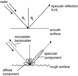
A perfectly smooth and flat conducting surface will act as a mirror, producing a coherent forward reflection, with the angle of incidence equal to the angle of reflection. However, if the surface has some roughness, the forward scatter component (called coherent or specular reflection) is reduced by diffuse, non-coherent scattering in other directions. For monostatic radar, clutter is the diffuse backscatter in the direction towards the radar. This is illustrated in Figure 11.1.
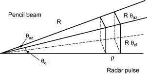
The magnitude of the backscattered signal is characterized by the normalized radar cross-section ![]() . At some instance during the propagation of the pulse, a pulsed radar will illuminate a patch on the surface, defined (for low grazing angles) to a first order by the pulse length, the antenna azimuth beamwidth and the local grazing angle. The backscatter from land or sea is then modeled assuming multiple scatterers distributed spatially uniformly over this clutter patch. This is illustrated in Figure 11.2.
. At some instance during the propagation of the pulse, a pulsed radar will illuminate a patch on the surface, defined (for low grazing angles) to a first order by the pulse length, the antenna azimuth beamwidth and the local grazing angle. The backscatter from land or sea is then modeled assuming multiple scatterers distributed spatially uniformly over this clutter patch. This is illustrated in Figure 11.2.

The normalized clutter reflectivity, ![]() , is defined as the total RCS,
, is defined as the total RCS, ![]() , of the scatterers in the illuminated patch, normalized by the area,
, of the scatterers in the illuminated patch, normalized by the area, ![]() , of the patch:
, of the patch:
![]() (11.1)
(11.1)
![]() is usually defined in units of
is usually defined in units of ![]() (dB relative to
(dB relative to ![]() radar cross-section, per
radar cross-section, per ![]() of area). Referring to Figure 11.2, the area of the clutter patch is given by
of area). Referring to Figure 11.2, the area of the clutter patch is given by
![]() (11.2)
(11.2)
where ![]() is the antenna azimuth beamwidth and
is the antenna azimuth beamwidth and ![]() is the local grazing angle. The range resolution,
is the local grazing angle. The range resolution, ![]() , is related to the radar pulse bandwidth, B, by
, is related to the radar pulse bandwidth, B, by ![]() , where c is the velocity of light. The factor
, where c is the velocity of light. The factor ![]() accounts for the actual compressed pulse shape and the azimuth beamshape, including the range and azimuth sidelobes. For a rectangular shaped pulse and beamshape,
accounts for the actual compressed pulse shape and the azimuth beamshape, including the range and azimuth sidelobes. For a rectangular shaped pulse and beamshape, ![]() , while for a Gaussian-shaped beam and rectangular pulse,
, while for a Gaussian-shaped beam and rectangular pulse, ![]() .
.
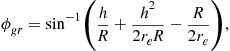
The grazing angle is defined in terms of the average local surface. For a nominally average flat surface, such as the sea, the grazing angle can be defined in terms of the radar height and propagation over a curved earth. In this case, the grazing angle, ![]() , can be written as:
, can be written as:
 (11.3)
where h is the height (altitude) of the radar, ![]() is the effective Earth’s radius and R is the slant range. For routine calculations at sea level,
is the effective Earth’s radius and R is the slant range. For routine calculations at sea level, ![]() , where r is the true earth radius. This allows for the effects of atmospheric refraction for a typical refractive index profile. The actual effective grazing angle will depend on the local propagation and may be greatly changed under conditions of anomalous propagation, such as a surface ducts [2]. Over land, the local grazing angle will often be dominated by the terrain elevation and slope, which must be determined for specific cases.
, where r is the true earth radius. This allows for the effects of atmospheric refraction for a typical refractive index profile. The actual effective grazing angle will depend on the local propagation and may be greatly changed under conditions of anomalous propagation, such as a surface ducts [2]. Over land, the local grazing angle will often be dominated by the terrain elevation and slope, which must be determined for specific cases.
The above expressions apply at low grazing angles, when the illuminated patch is defined by the azimuth beamwidth and pulse length. At high grazing angles, or for low bandwidth radars, the illuminated patch may be defined by the antenna azimuth and elevation beamwidths. Care should be taken if the grazing angle varies significantly over the illuminated patch, as ![]() will not be constant.
will not be constant.
2.11.2.1.2 Clutter volume reflectivity
A similar approach is taken for volume scattering. This is defined in terms of the volume reflectivity, ![]() :
:
![]() (11.4)
(11.4)
with units of ![]() .
.
The illuminated volume, ![]() , is given approximately by:
, is given approximately by:
![]() (11.5)
(11.5)
where ![]() is the one-way 3 dB elevation beamwidth. This is illustrated in Figure 11.3.
is the one-way 3 dB elevation beamwidth. This is illustrated in Figure 11.3.
Clearly, this expression for the illuminated volume assumes that the volume scatterers fully fill the antenna beam and pulse length at a given range. If this is not the case, appropriate corrections must be made. For example, a volume search radar may have a narrow azimuth beam and a broad elevation beam. When illuminating rain, the rain ceiling may subtend a smaller angle than the upper edge of the beam.
2.11.2.1.3 Amplitude statistics
As illustrated in Figures 11.2 and 11.3, the return from clutter is usually assumed to comprise the backscatter from multiple scatterers, uniformly spatially distributed over an area or volume.
The scattered field, y, can be written as the vector sum from N random scatterers:
![]() (11.6)
(11.6)
where ![]() is the radar cross-section of a single scatterer,
is the radar cross-section of a single scatterer, ![]() is a phase term (related to the reflection coefficient and the relative range of each scatterer from the radar). Provided
is a phase term (related to the reflection coefficient and the relative range of each scatterer from the radar). Provided ![]() , the probability density function of the real and imaginary parts of y will be Gaussian, through the application of the central limit theorem (CLT). The corresponding PDFs for the envelope and intensity of the signal will be:
, the probability density function of the real and imaginary parts of y will be Gaussian, through the application of the central limit theorem (CLT). The corresponding PDFs for the envelope and intensity of the signal will be:
 (11.7)
where r is ![]() ,
, ![]() ,
, ![]() .
.
This representation of clutter is applicable to spatially uniform clutter observed with low-resolution radars (i.e., with a large clutter patch, so ![]() ). This may apply to sea clutter, observed at high grazing angles and low resolution, or to, say, large flat areas of monoculture on land, such as woods or fields.
). This may apply to sea clutter, observed at high grazing angles and low resolution, or to, say, large flat areas of monoculture on land, such as woods or fields.
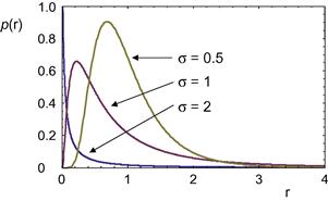
In many cases this representation is too simplistic. For example, the clutter mean intensity, ![]() above, may vary from one clutter cell to another, even though each cell still comprises multiple scatterers as in (11.6). Under these circumstances, the overall PDF will no longer have simple Gaussian statistics. Figure 11.4 illustrates the difference between returns with a Rayleigh PDF compared with clutter with strongly non-Gaussian statistics, modeled by a K distribution PDF, which is discussed below. A variation of the underlying mean intensity can be incorporated into the overall amplitude statistics by extending the simple model for PDF to include a dependence on the local mean intensity, which we shall call
above, may vary from one clutter cell to another, even though each cell still comprises multiple scatterers as in (11.6). Under these circumstances, the overall PDF will no longer have simple Gaussian statistics. Figure 11.4 illustrates the difference between returns with a Rayleigh PDF compared with clutter with strongly non-Gaussian statistics, modeled by a K distribution PDF, which is discussed below. A variation of the underlying mean intensity can be incorporated into the overall amplitude statistics by extending the simple model for PDF to include a dependence on the local mean intensity, which we shall call ![]() . Now:
. Now:
 (11.8)
The mean level ![]() is itself a random variable with PDF
is itself a random variable with PDF ![]() , so that the overall PDF can be written
, so that the overall PDF can be written
![]() (11.9)
(11.9)
This way we obtain the so-called compound-Gaussian model. The use of this type of model to represent radar sea clutter was originally described in [6–8]. The compound K distribution form of the model, discussed below, was originally formulated by Ward et al. [9,10]. There is further discussion in [9–21], and references therein. According to this model, each sample of the complex envelope of the sea clutter process is the product of two random variables: the texture and the speckle and can be represented as ![]() . The term
. The term ![]() represents a stationary complex Gaussian process, called speckle, which accounts for local backscattering;
represents a stationary complex Gaussian process, called speckle, which accounts for local backscattering; ![]() e
e![]() are the in-phase and quadrature components of the speckle complex envelope
are the in-phase and quadrature components of the speckle complex envelope ![]() . They satisfy the property
. They satisfy the property ![]() and
and ![]() , so that
, so that ![]() , i.e., the speckle complex samples have unit power. The factor
, i.e., the speckle complex samples have unit power. The factor ![]() is a non-negative real random process, called texture that, as said, models the local clutter power.
is a non-negative real random process, called texture that, as said, models the local clutter power.
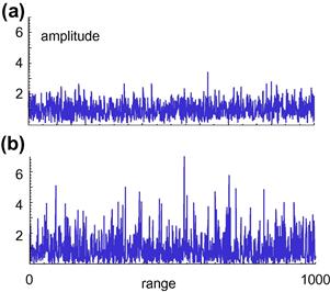
Figure 11.4 Envelope of uncorrelated signals versus time; (a) Rayleigh noise, mean level 1; (b) K distributed clutter, mean level 1, ![]() .
.
The compound-Gaussian model can be derived also as an extension of the CLT, allowing the number of scatterers N in Eq. (11.6) to be a random variable [16,22]. In the particular case in which the number of scatterers is distributed following a negative binomial PDF, the texture can be shown to be a Gamma-distributed random variable (r.v.), and the amplitude a K-distributed r.v. (see Eq. (11.10)).
The compound-Gaussian model counts among its particular cases some families of distribution that are very popular in clutter modeling. The analytical expressions for these PDFs and their moments ![]() are reported below, where
are reported below, where ![]() denotes the clutter amplitude.
denotes the clutter amplitude.
K-model (K):
Replacing in Eq. (11.9) the generic ![]() with the Gamma PDF
with the Gamma PDF ![]() , we obtain
, we obtain
 (11.10)
![]() (11.11)
(11.11)
where ![]() is the gamma function,
is the gamma function, ![]() is the modified Bessel function of the second kind, of order
is the modified Bessel function of the second kind, of order ![]() is the shape parameter, and
is the shape parameter, and ![]() is the mean.
is the mean.
Generalized K model with lognormal texture (LNT):
 (11.12)
 (11.13)
where ![]() is the shape parameter, and m is the scale parameter. This model cal be obtained with the lognormal texture PDF
is the shape parameter, and m is the scale parameter. This model cal be obtained with the lognormal texture PDF ![]() .
.
Generalized K model with generalized Gamma texture (GK):
Putting in Eq. (11.9) the generalized Gamma texture PDF ![]() we obtain
we obtain
 (11.14)
![]() (11.15)
(11.15)
Weibull model (W):
![]() (11.16)
(11.16)
![]() (11.17)
(11.17)
where c is the shape parameter and b is the scale parameter. The Rayleigh PDF is a particular case of the Weibull PDF for c = 2 [23]. Unfortunately, for the Weibull distribution, the PDF of the texture does not have a closed form and it is a compound-Gaussian model only for c < 2 [12].
Other sources of variability in clutter give rise to non-Gaussian statistics. While compound distributions can give some insight into the physical model underlying the non-Gaussian behavior, it is often sufficient to find an empirical fit of the overall amplitude statistics to a generalized PDF. Other popular distributions include the lognormal model, which does not belong to the compound-Gaussian family. The expressions of PDF and the moments are given below.
Lognormal model (LN):
![]() (11.18)
(11.18)
![]() (11.19)
(11.19)
where ![]() is the shape parameter, and
is the shape parameter, and ![]() is the scale parameter and
is the scale parameter and ![]() the unit step function. Unfortunately, the LN model does not satisfies any of the compound-Gaussian properties [12].
the unit step function. Unfortunately, the LN model does not satisfies any of the compound-Gaussian properties [12].
The non-Gaussian PDFs K, W, and LN each have two parameters, a shape and a scale parameter, that can be adjusted to fit the observed data. The GK, conversely, has three parameters. Figures 11.5–11.7 illustrate examples of PDFs from different families.


The K and Weibull distributions are very similar, both including the Rayleigh distribution as part of their family (![]() in the Weibull distribution and
in the Weibull distribution and ![]() in the K distribution) and they are often used for sea clutter modeling. The lognormal distribution gives PDFs with much longer tails (i.e., a higher probability of achieving larger amplitudes relative to the mean amplitude). This is often used for modeling land clutter, when the presence of large discrete scatterers can give rise to long tails if they are included in distributed clutter. A model that explicitly includes discrete spikes is the KA distribution, which is described in detail in [24,25].
in the K distribution) and they are often used for sea clutter modeling. The lognormal distribution gives PDFs with much longer tails (i.e., a higher probability of achieving larger amplitudes relative to the mean amplitude). This is often used for modeling land clutter, when the presence of large discrete scatterers can give rise to long tails if they are included in distributed clutter. A model that explicitly includes discrete spikes is the KA distribution, which is described in detail in [24,25].
2.11.2.1.4 Doppler spectrum
The simple model for clutter scattering given by (11.6), does not include any variation over time. If the individual clutter scatterers are moving radially with respect to the radar, the phase will vary with time, so that
![]() (11.20)
(11.20)
Assuming random motion of the scatterers, the temporal variations of the return must be described in terms of the autocorrelation function, ACF:
![]() (11.21)
(11.21)
The power spectrum of the returns can be related to the ACF from its Fourier transform (Weiner Khintchine theorem):
![]() (11.22)
(11.22)
where ![]() is the Doppler radian frequency and
is the Doppler radian frequency and ![]() , where f is the Doppler frequency.
, where f is the Doppler frequency.
The Doppler power spectrum (power spectral density PSD) is often modeled as having a Gaussian shape:
 (11.23)
This is usually a mathematical convenience rather than any attempt at realism. Often the Doppler spectrum will be strongly asymmetric and the mean Doppler shift, ![]() , may not be zero. Clearly for land clutter
, may not be zero. Clearly for land clutter ![]() is usually zero, but for rain and sea clutter in general
is usually zero, but for rain and sea clutter in general ![]() and will be dependent on the wind speed and direction. Moreover, for sea clutter, as first reported by Pidgeon at C-band [26], and in X-band [27], the sea spectrum exhibits different peaks in the HH and VV polarizations [28,25,10]. Generally the spectral component corresponding to the lower frequency peak relative to the VV polarization, associated with the Bragg scattering component, is well described by the Gaussian function (11.23). On the contrary, the HH polarization is characterized by a higher frequency peak in the spectrum, maybe owing to the scattering from fast moving (faster than Bragg scatterers) and short-life scatterers. In this polarization the clutter PSD is well described by the Lorentzian function (autoregressive model of order 1)
and will be dependent on the wind speed and direction. Moreover, for sea clutter, as first reported by Pidgeon at C-band [26], and in X-band [27], the sea spectrum exhibits different peaks in the HH and VV polarizations [28,25,10]. Generally the spectral component corresponding to the lower frequency peak relative to the VV polarization, associated with the Bragg scattering component, is well described by the Gaussian function (11.23). On the contrary, the HH polarization is characterized by a higher frequency peak in the spectrum, maybe owing to the scattering from fast moving (faster than Bragg scatterers) and short-life scatterers. In this polarization the clutter PSD is well described by the Lorentzian function (autoregressive model of order 1)
![]() (11.24)
(11.24)
where the constant k depends on the mean lifetime of scatterers.
In some practical situations the above-mentioned two models do not suffice to fit the real spectra shape, especially for the HH polarization. In [28] the authors consider first the scattering from fast-to-intermediate scatterers (e.g., bound-Bragg waves, etc.) whose PSD is characterized by a convolution of the Gaussian and Lorentzian profiles, resulting in the Voigtian function, and then a linear combination of these three models to improve the fitting.
Another simple model often used for both sea and land clutter PSD is the autoregressive (AR) one. The rationale for adopting AR models for the radar echoes is to have a highly parameterized model with a minimum number of parameters that can be easily estimated. Some examples can be found in [29,30].
For moving platforms, the antenna motion with respect to the clutter will also modify the Doppler spectrum. This is illustrated in Figure 11.8 for a side looking antenna, with one-way 3 dB beamwidth ![]() and platform velocity v. If the antenna has a Gaussian shape, the combined Doppler spectrum due to platform motion and internal clutter motion will be approximately:
and platform velocity v. If the antenna has a Gaussian shape, the combined Doppler spectrum due to platform motion and internal clutter motion will be approximately:
 (11.25)

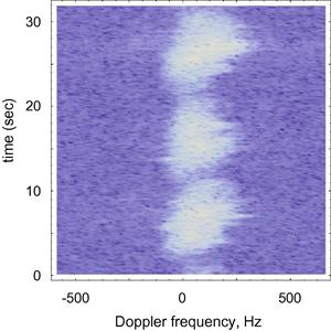
Figure 11.9 shows an example of the Doppler spectrum of sea clutter as function of time, derived from radar data collected by CSIR [31]. The radar was vertically polarized with a frequency of 9 GHz, a pulse repetition frequency, ![]() , of 5 kHz and a range resolution of 15 m. The local grazing angle for the data collected was approximately
, of 5 kHz and a range resolution of 15 m. The local grazing angle for the data collected was approximately ![]() . The radar look direction was
. The radar look direction was ![]() , with wind of 15 kts from
, with wind of 15 kts from ![]() and a wave direction of
and a wave direction of ![]() , significant wave height 2.2 m. The raw data was then processed over bursts of L = 512 samples with an FFT, using a −55 dB Dolph-Chebyshev weighting function in the time domain. It can be seen that the clutter intensity varies in time in a periodic manner. The spectrum width also varies with time, with occasional extreme Doppler excursions, such as seen around 27 s into the time record, perhaps as the result of local wind gusting. Finally, the spectrum appears asymmetric in shape, with a non-zero mean Doppler shift. These features highlight the complexity of the relationship between the intensity modulation and the form of the spectrum, the former being dominated by the swell structure in the sea surface and the latter being additionally affected by the local gusting of the wind and the detailed scattering mechanism. This non-stationary behavior of sea clutter will be addressed with more detail in Section 2.11.3.1.7. However, despite this complexity it should be noted that the compound modulated Gaussian process is still applicable in the spectral domain and will affect the performance of both coherent and non-coherent radars.
, significant wave height 2.2 m. The raw data was then processed over bursts of L = 512 samples with an FFT, using a −55 dB Dolph-Chebyshev weighting function in the time domain. It can be seen that the clutter intensity varies in time in a periodic manner. The spectrum width also varies with time, with occasional extreme Doppler excursions, such as seen around 27 s into the time record, perhaps as the result of local wind gusting. Finally, the spectrum appears asymmetric in shape, with a non-zero mean Doppler shift. These features highlight the complexity of the relationship between the intensity modulation and the form of the spectrum, the former being dominated by the swell structure in the sea surface and the latter being additionally affected by the local gusting of the wind and the detailed scattering mechanism. This non-stationary behavior of sea clutter will be addressed with more detail in Section 2.11.3.1.7. However, despite this complexity it should be noted that the compound modulated Gaussian process is still applicable in the spectral domain and will affect the performance of both coherent and non-coherent radars.
2.11.2.1.5 Polarization characteristics
It is observed that most clutter characteristics are very dependent on the polarization of the radar signal and so an understanding of polarization is important.
A wave is said to be polarized if the direction of the electric, E, and magnetic, H, fields reside in a fixed plane. The plane in which the E vector moves is called the plane of polarization. The polarization scattering matrix, S, describes the amplitude and relative phase of returns from different combinations of polarizations on transmit and receive:
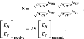 (11.26)
where:
![]() , RCS for Tx on H and Rx on H polarization;
, RCS for Tx on H and Rx on H polarization;
![]() , RCS for Tx on V and Rx on V polarization;
, RCS for Tx on V and Rx on V polarization;
For monostatic backscatter ![]() and
and ![]() .
.
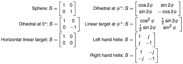
The discussion above is for linear polarization and some examples of polarization scattering matrices for different targets types are shown in Table 11.1. Similar matrices can be used to describe the relationship for circular polarized signals (right or left handed) or any orthogonal coordinate system.
If the V and H components of the electric field are in phase, linear polarization is obtained. In general, an arbitrary phase between the V and H fields produces an elliptical polarization. The special case of a ![]() phase shift gives circular polarization.
phase shift gives circular polarization.
For circular polarization, left-hand polarization is defined when ![]() on transmit; right-hand polarization is defined with
on transmit; right-hand polarization is defined with ![]() .
.
The circular-polarization scattering matrix is defined as
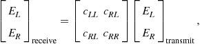 (11.27)
while the linear-polarization has a scattering matrix given by
 (11.28)
The circular polarization RCS terms can then be related to the linear polarization RCS terms by:
 (11.29)
Using the definitions above, it can be seen that for a sphere, where ![]() and
and ![]() :
:
![]() (11.30)
(11.30)
For this reason circular polarization is often used to reduce the return from rain clutter. Odd-bounce scatterers such as spheres or trihedrals will reverse the hand of polarization on reflection and a perfect sphere will have ![]() . Unfortunately, raindrops are not perfectly spherical but, even so, the reflectivity of rain may be reduced by about 15 dB to as much as 30 dB, dependent on conditions.
. Unfortunately, raindrops are not perfectly spherical but, even so, the reflectivity of rain may be reduced by about 15 dB to as much as 30 dB, dependent on conditions.
Target signatures, such as high-resolution range profiles, may be quite different according to polarization. For example using circular polarization, ![]() will show odd bounce scatterers while
will show odd bounce scatterers while ![]() will show even bounce scatterers.
will show even bounce scatterers.
2.11.2.1.6 Spatial correlation
The returns from spatially uniform clutter will have Gaussian amplitude statistics, as described in Section 2.11.2.1.3. The magnitude of the return will change as the viewing geometry changes, such as when the antenna beam scans in azimuth or the range from the radar is changed. For a square beam and pulse shape (see Section 2.11.2.1.2), the returns from clutter patches spaced by more than one beamwidth or one pulse length will be independent and uncorrelated. However, if the successive clutter patches overlap spatially, then the returns will be correlated. A convenient measure of the spatial correlation of a sequence of intensity samples, ![]() is given by the estimation of the correlation coefficient:
is given by the estimation of the correlation coefficient:
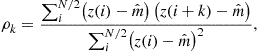 (11.31)
where ![]() is an estimate of the mean intensity and k is the correlation lag
is an estimate of the mean intensity and k is the correlation lag ![]() . For spatially uniform clutter with Gaussian statistics and a fractional overlap of the beam or pulses between successive samples of
. For spatially uniform clutter with Gaussian statistics and a fractional overlap of the beam or pulses between successive samples of ![]() , then the correlation coefficient of the clutter intensity is
, then the correlation coefficient of the clutter intensity is ![]() .
.
Spatial correlation of the clutter returns may also be observed if the local normalized reflectivity is changing in a systematic way. One example of this is observed over the short term in sea clutter, when the spatial variations caused by the sea swell or waves causes a related variation in the local mean reflectivity. This is illustrated in Section 2.11.3.1. Some examples of the range profiles of the local mean intensity of sea clutter and their corresponding range correlation coefficients are shown in Figure 11.10.

Figure 11.10 Recorded data exhibiting different spatial correlations. Reproduced with permission from [25] © The Institution of Engineering and Technology.
2.11.2.1.7 Discrete scatterers
The models for spatially distributed clutter are very useful for representing the returns from rain and often from land and sea, especially at high grazing angles. However, under some conditions the underlying assumptions of spatially uniform scatterers is no longer valid. For example, at low grazing angles terrain scattering may become very patchy and spiky, and is dominated by local high structures [32]. At higher grazing angles a distributed clutter model for terrain becomes more useful, but there will often also be a number of very large discrete scatterers in any scene, due to natural and man-made features. Barton [33] has analyzed a number of results from the literature and suggests that discrete clutter echoes of ![]() RCS might have a typical density of
RCS might have a typical density of ![]() RCS a density of
RCS a density of ![]() ; and
; and ![]() RCS a density of
RCS a density of ![]() . Discrete scatterers as large as
. Discrete scatterers as large as ![]() RCS may be found. Long [34] suggest a density of about
RCS may be found. Long [34] suggest a density of about ![]() for
for ![]() RCS and
RCS and ![]() for
for ![]() RCS.
RCS.
Sea clutter may also include discrete spikes that have distinctly different properties from the surrounding clutter. In particular, specular scattering with HH polarization from the crests of incipient breaking waves may give rise to very localized returns having a large RCS [25]. The KA distribution [24,25] can be used to model discrete spikes that are added to the standard compound K distribution model. The amplitude distribution of clutter spikes has also been investigated in [35] who used the KK distribution to achieve a good fit to the tail of the distribution of clutter-plus-noise data recorded at medium grazing angles.
2.11.2.2 Sea clutter
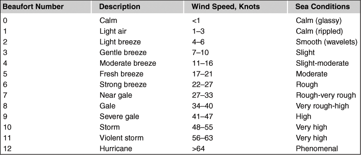
Observations of radar sea clutter are usually associated with particular characteristics of the sea surface and environment, such as sea waves, sea swell and wind speed. Sea waves are the interaction between the wind and the sea surface. As the wind blows over the surface, waves are generated that increase in height and wavelength over time. Eventually an equilibrium is reached when the energy dissipated in the waves matches the energy input by the wind. This allows an average wave height to be associated with a specific wind speed, provided that the duration (the length of time that the wind has been blowing at a given speed) and the fetch (the range extent over which the wind has been blowing) are known. Wave heights are usually measured in terms of ![]() , the specific wave height, defined at the average peak to trough wave height of the highest one third of the waves. Ranges of significant wave heights are associated with different sea states, which can be associated with wind speed, as discussed above. Table 11.2 shows the relationships for the Douglas sea state, which is usually used for radar sea clutter modeling. Wind speed is usually characterized in terms of the Beaufort wind scale, which is shown in Table 11.3.
, the specific wave height, defined at the average peak to trough wave height of the highest one third of the waves. Ranges of significant wave heights are associated with different sea states, which can be associated with wind speed, as discussed above. Table 11.2 shows the relationships for the Douglas sea state, which is usually used for radar sea clutter modeling. Wind speed is usually characterized in terms of the Beaufort wind scale, which is shown in Table 11.3.

It should be noted that assessing the environment in a particular trial is notoriously difficult and the sea state reported by observers can show a wide variation. Wave-rider buoys can be used to estimate local wave heights but these can usually only gave a rough guide to likely clutter characteristics, which depend on things such as the “wind friction velocity,” “ wave age” and so on. These issues are discussed in detail in [25].
2.11.2.2.1 Theoretical and empirical models for sea clutter reflectivity
The radar backscatter from the sea is derived from a complex interaction between the incident electromagnetic waves and the sea surface. There are many theoretical models for backscatter, based on the physics of scattering from rough surfaces and approximations to scattering mechanisms. The simplest models attempt to represent the surface as many small segments, called facets, with orientations modulated by the waves. Scattering from wind-driven ripples may be approximated by Bragg scattering. The tilting of the ripples by longer sea waves changes the scattered power. This type of model, introduced by Wright [36] and Bass et al. [37], is discussed in detail in [25] and can give good results at medium to high grazing angles. However, at low grazing angles and high sea states the electromagnetic scattering becomes much more complex, with multiple reflection paths and shadowing from adjacent waves. There will also be breaking waves that can contribute considerably to the backscatter and are not modeled by simple modulated Bragg scattering. Some progress has been made recently in the understanding of electromagnetic scattering at low grazing angles [25]. However, the practical development of sea clutter models still mainly relies on empirical measurements.
Figure 11.11 shows a typical plot of normalized clutter reflectivity, ![]() , for sea clutter as a function of grazing angle, for VV and HH polarizations. At near vertical incidence, the backscatter is quasi-specular. In this region, the backscatter varies inversely with surface roughness with maximum backscatter at vertical incidence for a perfectly smooth surface. At medium grazing angles the reflectivity shows a lower dependence on grazing angle. This is often called the plateau region. Here the reflectivity is well modeled by the composite model. Below some critical angle (typically around
, for sea clutter as a function of grazing angle, for VV and HH polarizations. At near vertical incidence, the backscatter is quasi-specular. In this region, the backscatter varies inversely with surface roughness with maximum backscatter at vertical incidence for a perfectly smooth surface. At medium grazing angles the reflectivity shows a lower dependence on grazing angle. This is often called the plateau region. Here the reflectivity is well modeled by the composite model. Below some critical angle (typically around ![]() grazing angle, dependent on the roughness) it is found that the reflectivity reduces much more rapidly with smaller grazing angles. This is known as the interference region, where propagation is strongly affected by multipath scattering and shadowing. Also shown in Figure 11.11 is the dependence of the reflectivity on radar polarization. In the plateau region, the backscatter for HH polarization is significantly lower than for VV polarization. This is evident of the significantly different scattering mechanisms for VV and HH polarizations.
grazing angle, dependent on the roughness) it is found that the reflectivity reduces much more rapidly with smaller grazing angles. This is known as the interference region, where propagation is strongly affected by multipath scattering and shadowing. Also shown in Figure 11.11 is the dependence of the reflectivity on radar polarization. In the plateau region, the backscatter for HH polarization is significantly lower than for VV polarization. This is evident of the significantly different scattering mechanisms for VV and HH polarizations.

Figure 11.11 Typical variation with grazing angle and polarization of sea clutter reflectivity at X-band (for a wind speed of about 15 km). Reproduced with permission from [25] © The Institution of Engineering and Technology.
In addition to a dependence on polarization and grazing angle, it is found that the reflectivity is strongly dependent on wind speed, which creates local surface roughness. This is often associated with the sea state but it should be noted that a strong sea swell in the absence of local wind may have a low reflectivity, while a strong wind may create a high reflectivity from a comparatively flat sea. The reflectivity will also depend to some extent on radar frequency. Another important consideration is propagation effects, such as ducting, which can change the local grazing angle of the signal incident on the sea surface. Indeed, observation of variation of surface reflectivity may be used to infer the presence of ducts [38].
There are various empirical models for the normalized clutter reflectivity that are used by radar designers. Tables of ![]() for different radar frequencies, grazing angles and sea states and for V and H polarizations are given in [1]. These values are the result of averaging measurements from many experiments. It may be noted that they do not model the variation of reflectivity with wind direction.
for different radar frequencies, grazing angles and sea states and for V and H polarizations are given in [1]. These values are the result of averaging measurements from many experiments. It may be noted that they do not model the variation of reflectivity with wind direction.
Another useful model, known as the GIT model [39], was developed by workers at the Georgia Institute of Technology in the 1970s. This model covers radar frequencies from 1 to 100 GHz and grazing angles from 0.1 to ![]() . It is based on an underlying multipath model as well as more general trends observed in experimental data sets. The normalized reflectivities modeled for H and V polarizations,
. It is based on an underlying multipath model as well as more general trends observed in experimental data sets. The normalized reflectivities modeled for H and V polarizations, ![]() (H) and
(H) and ![]() (V), respectively, are given by the following expressions:
(V), respectively, are given by the following expressions:
Radar frequency 1–10 GHz
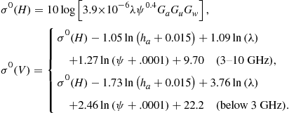 (11.32)
The adjustment factors are

Radar frequency 10–100 GHz
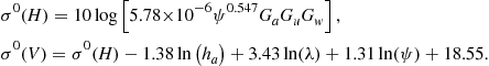 (11.33)
and the adjustment factors are

The units and symbols used here are:
![]() reflectivity for H and V polarizations, dB
reflectivity for H and V polarizations, dB![]()
![]() look direction relative to wind direction, rad
look direction relative to wind direction, rad
Radar performance is often specified in terms of sea state and a useful relationship between sea state, s, and wind speed for a fully developed sea is:
![]() (11.34)
(11.34)
Figures 11.12 and 11.13 show examples, using the GIT model, of ![]() and
and ![]() as a function of sea state and grazing angle, for the radar looking cross-wind and radar frequency 10 GHz (using Eq. (11.32)).
as a function of sea state and grazing angle, for the radar looking cross-wind and radar frequency 10 GHz (using Eq. (11.32)).

Figure 11.12 GIT model: ![]() as a function of grazing angle for sea states 1–6, for the radar looking cross-wind and radar frequency 10 GHz.
as a function of grazing angle for sea states 1–6, for the radar looking cross-wind and radar frequency 10 GHz.

Figure 11.13 GIT model: ![]() as a function of grazing angle for sea states 1–6, for the radar looking cross-wind and radar frequency 10 GHz.
as a function of grazing angle for sea states 1–6, for the radar looking cross-wind and radar frequency 10 GHz.
It may be noted that the values of normalized reflectivity given by the GIT model are significantly different from some of the values given in [1], especially at low grazing angles. This is not surprising, given that the models were derived from different data sets, and reflects the wide variation of values that may be encountered for nominally similar conditions.
2.11.2.2.2 Sea clutter amplitude statistics
Observation of the returns from the sea surface has identified two distinct components of the amplitude fluctuations. The first is a spatial variation, the texture, often associated with the sea swell. This represents a spatial and longer-term temporal variation of the local mean clutter level. This component de-correlates only slowly with time and is not affected by radar frequency agility. The second is a speckle component, associated with scattering from multiple scatterers in a given range cell. The speckle component de-correlates with time due to relative motion of the scatterers or due to changes in radar frequency.
These characteristics are shown in Figures 11.14 and 11.15 [25], which show recordings of radar sea clutter data, with a radar operating in X band (9 GHz), with a ![]() antenna beamwidth and 4.2 m range resolution.
antenna beamwidth and 4.2 m range resolution.
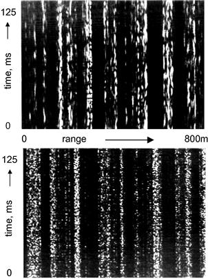
Figure 11.14 Range-time intensity plots of sea clutter; upper plot shows returns from a fixed frequency radar and lower plot shows returns with pulse-to-pulse frequency agility. Reproduced with permission from [25] © The Institution of Engineering and Technology.
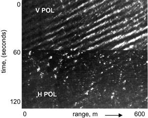
Figure 11.15 Range-time intensity plot of sea clutter averaged over 250 successive pulses to reduce the speckle component, revealing the underlying mean level. After 60 s, the radar was switched from vertical to horizontal polarization. Reproduced with permission from [25] © The Institution of Engineering and Technology.
Figure 11.14 shows range-time intensity plots of returns for a range interval of 800 m and a period of 125 ms, with a PRF of 1 kHz. The radar range was 5 km and the grazing angle was ![]() . The upper part of the figure shows fixed frequency returns. At a given range the returns exhibit a correlation time of
. The upper part of the figure shows fixed frequency returns. At a given range the returns exhibit a correlation time of ![]() . The underlying swell pattern is clearly visible. The lower figure shows frequency agile returns. Now returns at each range are decorrelated from pulse to pulse but the swell pattern is not affected.
. The underlying swell pattern is clearly visible. The lower figure shows frequency agile returns. Now returns at each range are decorrelated from pulse to pulse but the swell pattern is not affected.
In Figure 11.15, the fluctuating component (speckle) has been reduced by adding successive pulses. After 60 s the polarization changes from VV to HH. The VV POL returns show a clear swell-like component while the HH POL returns show short lived ![]() clutter “spikes” which still appear to be associated with the swell peaks. It may also be noted that the overall mean level of the HH returns appears to be lower than that of the VV returns, evidence of a lower reflectivity,
clutter “spikes” which still appear to be associated with the swell peaks. It may also be noted that the overall mean level of the HH returns appears to be lower than that of the VV returns, evidence of a lower reflectivity, ![]() .
.
Using data of the type shown in Figure 11.15, it has been shown [10] that the distribution of the local mean power fits well to the Gamma distribution. The local scattering (at a given range in Figure 11.14) has Gaussian statistics, resulting in the envelope of the overall return having the compound form of the K distribution (11.10). An empirical model for the dependence of the shape parameter ![]() on radar, environmental and geometric parameters has been developed through the analysis of experimental data at X-band (9–10 GHz). The model is [25]:
on radar, environmental and geometric parameters has been developed through the analysis of experimental data at X-band (9–10 GHz). The model is [25]:
![]() (11.35)
(11.35)
where
![]() is the grazing angle in degrees,
is the grazing angle in degrees,
![]() is a polarization dependent parameter (1.39 for VV and 2.09 for HH), and
is a polarization dependent parameter (1.39 for VV and 2.09 for HH), and
(The last term is omitted if there is no swell).
There are no known comparable models for the shape parameters of the Weibull and Lognormal distribution models.
2.11.2.2.3 Sea clutter Doppler spectrum
The Doppler spectrum of sea clutter varies with environmental condition, just as do the values of ![]() and the amplitude statistics. A useful simple low grazing angle model [40] for the shape of the average clutter velocity spectrum upwind at a given wind speed
and the amplitude statistics. A useful simple low grazing angle model [40] for the shape of the average clutter velocity spectrum upwind at a given wind speed ![]() is a Gaussian shape with a mean velocity of
is a Gaussian shape with a mean velocity of ![]() and standard deviation of
and standard deviation of ![]() given by (in
given by (in ![]()
 (11.36)
where (VV) and (HH) denote the values for vertical and horizontal polarizations, respectively. This model can be applied to Eq. (11.23) with ![]() and
and ![]() .
.
There are many observations from data that can be used to improve this simple model. As the radar scans away from upwind, the mean velocity changes approximately proportionately with the view direction component of the wind vector, while the standard deviation remains approximately unchanged. The shape of the spectrum is skewed somewhat in the direction of the wind, and the shape varies in a complicated manner as the local mean power in the compound K distribution changes [41,42]. This is dependent on polarization and sea conditions. It causes the shape parameter of the magnitude distributions in individual frequency filters (after Doppler radar processing) to vary with frequency [10,42,43], thus causing difficulties for false alarm rate control in Pulsed Doppler and MTI radar systems. More research is needed to develop quantitative models to characterize these effects.
2.11.2.3 Ground clutter
Land (or ground) clutter is the most difficult to characterize of the common clutter categories. It can rarely be described as spatially uniform except perhaps for local regions of woods, open fields or desert. Almost invariably there are abrupt changes in clutter due to natural or man-made boundaries (river banks, hedges, edges of woods, etc.), significant local variation in ground slope and many isolated discrete scatterers (rocks, isolated trees, pylons, buildings). Urban environments are particularly complex, as might be expected.
For modeling convenience and mathematical tractability ground clutter is often modeled quite simply as uniformly distributed scatters over a “flat” earth. Of course, amplitude statistics over large areas of land are most unlikely to be described by single Gaussian statistics with a steady backscatter power. If the backscatter coefficient is taken as representing the global mean backscatter, amplitude distributions such as the K-distribution or Log-Normal distribution are often used to fit to measured data. More detailed modeling of backscatter from land usually requires modeling of specific sites. An excellent reference for a very detailed exposition of the nature and statistics of land clutter has been written in [32]. Further useful sources of data are to be found in [2,33,44–47].
2.11.2.3.1 Empirical models of  for land clutter
Normalized clutter RCS,  , at low grazing angles
At low grazing angles the returns from land clutter become very spiky. Shadowing due to terrain height variations and cultural features become very marked. Under these conditions, it becomes very difficult to distinguish between spiky distributed clutter and discrete scatterers, whether man-made or natural. An excellent source of empirical measurements is the work at the MIT Lincoln Laboratory by Billingsley and others [32]. This has resulted in a very large database of land clutter data for a wide variety of terrain at low grazing angles. Measurements were made at 42 sites across North America at frequencies ranging from VHF (167 MHz) to X-band (9.2. GHz). Range resolutions of 150 m and either 36 m or 15 m were used, with both vertical and horizontal polarizations. However, Billingsley reported that variations in reflectivity due to polarization and resolution were small (1–2 dB). Because of the difficulty of defining the local grazing angle in uneven terrain, the depression angle from the radar was recorded, taking into account the earth curvature but not the effect of local terrain slope. Billingsley reported that for very low grazing angles, where masking occurs, the amplitude statistics can be represented by the Weibull PDF. At higher grazing angles, with less masking, the clutter backscatter increases and for depression angles above about ![]() the clutter can be represented by a Rayleigh PDF.
the clutter can be represented by a Rayleigh PDF.
Another useful empirical model was developed at the Georgia Institute of Technology [48]. This model provides an empirical fit to clutter reflectivity for a range of different terrains and radar frequencies:
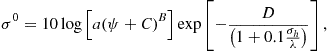 (11.37)
where
Table 11.4 shows values of the parameters A, B, C, and D given in [48].

Normalized clutter RCS—medium grazing angles
At medium grazing angles, more measurements of clutter are available, although ground truth is often difficult to obtain. It has been found that in the “plateau region” of backscatter (see Figure 11.11), the clutter reflectivity is approximately proportional to the sine of the grazing angle, ![]() (see Figure 11.2) leading to clutter normalized RCS being defined in terms of a parameter
(see Figure 11.2) leading to clutter normalized RCS being defined in terms of a parameter ![]()
![]() (11.38)
(11.38)
Typical values of ![]() have been reported by Barton [33], as summarized in Table 11.5.
have been reported by Barton [33], as summarized in Table 11.5.

Other empirical models for land clutter can be found in [46–49].
2.11.2.4 Rain clutter
Backscatter from rain and other precipitation, such as hail and snow, can have a significant effect on radar performance. In addition, for frequencies significantly above 9 GHz the attenuation of the radar signal can be considerable. A useful summary of the effects of precipitation and weather on radar is given by Nathanson [1].
As with other types of clutter, some progress has been made with theoretical modeling of electromagnetic scattering but in general radar designers resort to empirical models of precipitation clutter.
2.11.2.4.1 Atmospheric attenuation
A detailed description of the attenuation of radar signals by the atmosphere has been provided by Blake [50]. Atmospheric attenuation varies with altitude, radar frequency and humidity. The references give typical figures for attenuation through the whole troposphere, attenuation over paths at sea level and so on. A simple rule of thumb for two-way atmospheric attenuation, ![]() , at sea level for a frequency f GHz is given by:
, at sea level for a frequency f GHz is given by:
![]() (11.39)
(11.39)
2.11.2.4.2 Rain attenuation
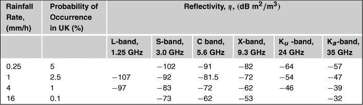
Rainfall is usually specified in terms of a rainfall rate, r, with the values for different levels of precipitation are given by Nathanson [1]:
The attenuation through rain is difficult to calculate theoretically, not least because conditions (humidity, drop size distribution and so on) can vary considerably for a nominal rainfall rate. Rainfall rates also vary with altitude and spatially across a given rainstorm. Again Nathanson [1] gives useful rules of thumb. The diameter, D, of a rainstorm can be represented by
![]() (11.40)
(11.40)
and if the rainfall rate at ground level is ![]() , the rate
, the rate ![]() at height h km, is given by:
at height h km, is given by:
![]() (11.41)
(11.41)
The attenuation of two-way radar signals through rain is approximated by:
![]() (11.42)
(11.42)
2.11.2.4.3 Theoretical and empirical model for rain reflectivity
Backscatter from rain can be modeled as scattering from multiple spheres. This is generally valid for small raindrops and theoretical models can be used to predict reflectivity, within their limits of validity. For higher rainfall rates (larger drops) these assumptions may no longer be valid and again the radar designer will resort to empirical models. For Rayleigh scattering from spherical drops ![]() , the volume reflectivity can be expressed as [2]:
, the volume reflectivity can be expressed as [2]:
 (11.43)
where D is the drop diameter, N is the number of drops, ![]() is the radar wavelength and
is the radar wavelength and ![]() , dependent on the dielectric constant and
, dependent on the dielectric constant and ![]() . It is found that
. It is found that
![]() (11.44)
(11.44)
where r is the rainfall rate in mm/h.
Empirical values for rain reflectivity are given by Nathanson [1], Currie [48], and Skolnik [2]. As an example, Table 11.6 shows some typical values of reflectivity given in [1]. Also shown in this table are values for the probability of different rainfall rates occurring, which is useful information when designing a radar for a particular application. The probabilities given in Table 11.6 are for the UK and values for other areas of the world can be found in [1].
2.11.2.4.4 Rain Doppler spectrum
The spectrum of wind-driven rain is of particular interest to radar designers. For radar meteorologists it provides detailed information on weather patterns. For weather avoidance radar on aircraft, Doppler provides important information on wind shear and other dangerous conditions.
A good discussion of the Doppler spectrum of rain is given in [1] and this is summarized here. The velocity spectrum and equivalent Doppler spectrum of rain clutter are conveniently modeled as having a Gaussian shape, with a standard deviations ![]() and
and ![]() , respectively. The spectrum of rain clutter is found to derive from various physical mechanisms, of which the principle ones are:
, respectively. The spectrum of rain clutter is found to derive from various physical mechanisms, of which the principle ones are:
• Wind shear, ![]() , caused by the variation of wind speed with height.
, caused by the variation of wind speed with height.
• Beam broadening, ![]() , caused by the variation in the radial velocity component of velocity across the radar beam.
, caused by the variation in the radial velocity component of velocity across the radar beam.
• Turbulence, ![]() , caused by turbulent atmospheric effects.
, caused by turbulent atmospheric effects.
• Fall velocity distribution, ![]() , caused by variations in raindrop fall velocities.
, caused by variations in raindrop fall velocities.
On the assumption that these spectral components are independent, the total velocity spectrum width can be given as:
![]() (11.45)
(11.45)
Figure 11.16 illustrates how wind shear contributes to variations in Doppler shift across the radar beam. Wind shear causes a change in wind velocity with height, which can be approximated as a constant velocity gradient with zero velocity at ground level. Across the elevation beam of a ground-based antenna there will be a linear change of radial velocity, ![]() , which for low elevation angles will equal the difference in horizontal wind speeds. For a Gaussian shaped beam:
, which for low elevation angles will equal the difference in horizontal wind speeds. For a Gaussian shaped beam:
![]() (11.46)
(11.46)
where k is the shear gradient (typical value ![]() , R is the range to the radar and
, R is the range to the radar and ![]() is the one-way 3 dB elevation beamwidth.
is the one-way 3 dB elevation beamwidth.

For altitudes up to about 3 km, ![]() . Beam broadening is due to tangential velocity variation across the antenna in azimuth and
. Beam broadening is due to tangential velocity variation across the antenna in azimuth and
![]() (11.47)
(11.47)
where ![]() is the tangential wind velocity at the beam centre,
is the tangential wind velocity at the beam centre, ![]() is the one-way antenna azimuth 3 dB beamwidth, and
is the one-way antenna azimuth 3 dB beamwidth, and ![]() is the azimuth angle relative to the wind direction at the beam centre.
is the azimuth angle relative to the wind direction at the beam centre. ![]() is usually only a small component of the spectrum.
is usually only a small component of the spectrum.
Finally, the distribution of vertical velocity amongst the raindrops will cause a spread in the velocity spectrum. A typical spread of vertical velocities is about ![]() so that at an elevation angle
so that at an elevation angle ![]() we have
we have
![]() (11.48)
(11.48)
2.11.3 Radar clutter analysis
For the effective application of theoretical models as presented in the previous Sections it is necessary to test their fit with real data using different radar parameters and environmental conditions. We have seen that a number of families of distributions can be used to fit the observed amplitude statistics over a wide range of conditions, including the log-normal, the Weibull and, especially, the compound-Gaussian model. The main goal of this section is to describe the statistical analysis performed on different experimental data of sea and land clutter, to comment on possible results and on the limitations of theoretical models in some conditions.
2.11.3.1 Sea clutter
Most of the results shown in this paragraph on sea clutter relate to the statistical analysis performed on the data recorded by IPIX radar during two campaigns, located in Dartmouth in 1993 and in Grimsby in 1998 [15,41,51]. Further extensive work on the modeling of sea clutter and the associated methods used for the statistical analysis of radar data are given in [25].
IPIX is an X-band (9.4 GHz) experimental instrumentation class radar, capable of dual polarized and frequency agile operation. During the first campaign, the radar site was located on a cliff facing the Atlantic Ocean, at a height of 100 ft above mean sea level and had an open view of about ![]() . During the second campaign it was on the shore of Lake Ontario, East of the “Place Polonaise” at Grimsby, between Toronto and Niagara Falls Ontario, looking at Lake Ontario from a height of 20 m.
. During the second campaign it was on the shore of Lake Ontario, East of the “Place Polonaise” at Grimsby, between Toronto and Niagara Falls Ontario, looking at Lake Ontario from a height of 20 m.
The data of Dartmouth are stored as 8 bits integers. For the second campaign, the radar was upgraded to a dynamic range of 10 bits (instead of 8 bits), so that strong target and weak clutter signals could be observed simultaneously without clipping or large quantization error. There are always like-polarizations, HH and VV (Lpol) and cross-polarizations, HV and VH (Xpol), coherent reception, leading to a quadruplet of in-phase and quadrature values for Lpol and Xpol (see Table 11.7).
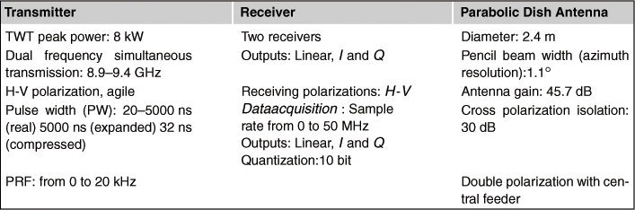
For the results shown in the following, the clutter data were collected during the Grimsby campaign. Many files with different range resolutions and recorded in different days have been analyzed [51], but here we summarize the results relating to only five files recorded on February 4, 1998 at about 22.30 h (local time) as representative of most of the results obtained from all the processed data. Unfortunately, there is no available information about the wind and wave observations for these datasets. The relevant parameters are summarized in Tables 11.8a and 11.8b.
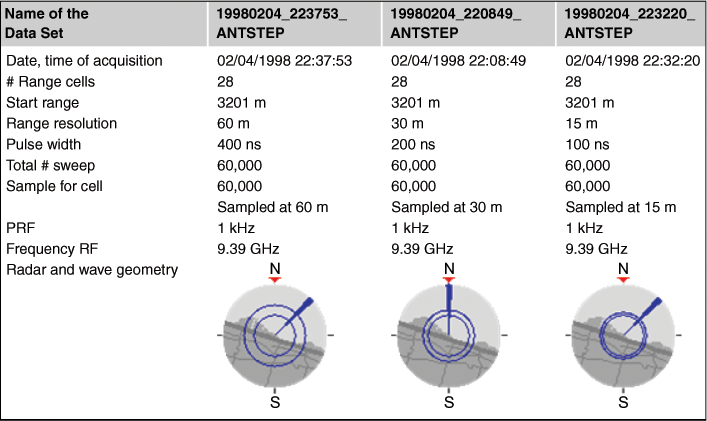

It is important to observe that in each file the range resolution is different, with data collected at 60 m, 30 m, 15 m, 9 m, and 3 m range resolution. The analysis here is aimed at highlighting the differences in clutter characteristics due to the change in the resolution.
The IPIX receiver has two operational modes depending upon the selected RF pulse width (PW). When the system was operating with ![]() , a 5 MHz filter was used to limit the receiver bandwidth to approximately 5 MHz. When
, a 5 MHz filter was used to limit the receiver bandwidth to approximately 5 MHz. When ![]() this filter was by-passed, so the bandwidth of the receiver was about 50 MHz to match the minimum 20 ns pulse width. Therefore, for data collected with
this filter was by-passed, so the bandwidth of the receiver was about 50 MHz to match the minimum 20 ns pulse width. Therefore, for data collected with ![]() , the receiver thermal noise level is about 10 dBs higher than for data collected with
, the receiver thermal noise level is about 10 dBs higher than for data collected with ![]() [52]. In the following figures the amplitude of the clutter is expressed in Volt (V).
[52]. In the following figures the amplitude of the clutter is expressed in Volt (V).
2.11.3.1.1 Statistical models of clutter amplitude
As already said, many distributions are described in the literature to model the amplitude probability density function (PDF) of high-resolution non-Gaussian clutter. Here we compare the empirical PDF with lognormal (LN), Weibull (W), K, and Generalized K (GK) and Generalized K with lognormal texture (LNT) PDFs whose expressions are given in Section 2.11.2.1.3.
The characteristic parameters of the theoretical PDFs can be estimated by the classical method of moments (MoM) [53], which consists of equating experimental moments with the corresponding theoretical moments. The estimated moments are given by:
 (11.49)
For the data at hand, ![]() samples have been processed for each range cell.
samples have been processed for each range cell.
Range resolutions of 60 m, 30 m, and 15 m
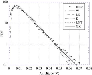
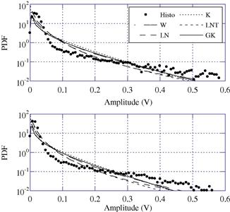
The results of the statistical analysis by means of histograms and estimated moments reveal that the GK-PDF yields a good fit for both co- and cross-polarized data and for all the three resolutions. Therefore, the analyzed clutter process can be accurately modeled by a compound-Gaussian process with Generalized K-PDF, provided that the size of the range resolution cell is greater than or equal to 15 m (note that the Gaussian model is a particular case of the Generalized K model).
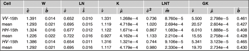
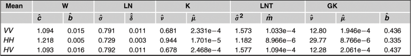
In Figures 11.17 and 11.18, we report the histogram and the moments for the 15th range cell, VV data, and 60 m range resolution. The numerical results for the other range cells and the two other range resolutions are very similar [51].

In Table 11.9 we report the mean values of the parameters estimated for each theoretical PDF. The results show that, for a resolution of 60 m, on the average, the HH component is spikier ![]() than both VV
than both VV![]() and VH
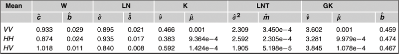
and VH![]() components.1 Moreover, the parameters estimated when the range resolution is 30 m (Table 11.10) show that the data are spikier at 30 m range resolution than at 60 m; this was found for all polarizations. The results show also that VV data
components.1 Moreover, the parameters estimated when the range resolution is 30 m (Table 11.10) show that the data are spikier at 30 m range resolution than at 60 m; this was found for all polarizations. The results show also that VV data ![]() and VH data
and VH data ![]() are spikier than HH data
are spikier than HH data ![]() .
.
For the range resolution of 15 m and for co-polarizations generally the GK-model provides a good fit to the data. The values of the estimated parameters confirm that the clutter gets spikier when range resolution increases (i.e., the size of the resolution cell decreases). We can also notice that on the average HH data are spikier ![]() than VV data
than VV data ![]() and VH data
and VH data ![]() ; the same happens for the 15 m resolution data (see Table 11.11).
; the same happens for the 15 m resolution data (see Table 11.11).
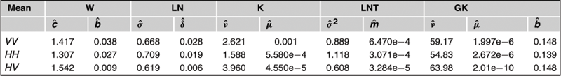
Range resolutions of 9 m and 3 m
Examining the histograms obtained by analyzing the file at a resolution of 9 m, it is possible to see that many cells of co-polarized data exhibit heavy-tails and none of the proposed models yields a good fit to the data. One of these cells is the fifth, plotted in Figure 11.19 for VV and HH data. This problem could be due to a non-Gaussian distribution of the speckle because of the very high range resolution. On the contrary, in [51] it was observed that for cross-polarizations, the clutter process can still be accurately modeled by a compound-Gaussian process with Generalized K-PDF. Again, the values of the estimated parameters show that HH data have the spikiest behavior (HH: ![]() , VV:
, VV: ![]() , VH:
, VH: ![]() , see Table 11.12).
, see Table 11.12).

The results obtained for co-polarizations at a range resolution of 3 m do not show significant differences with respect to the results obtained at 9 m. Conversely, the analysis for VH polarization presents some difference. There are cells showing histograms with tails longer than the average length recorded at lower resolutions; in this case the compound model cannot be used to model clutter data.
The estimates of the parameters are reported in Table 11.13. The results show again that HH data ![]() are spikier than VV
are spikier than VV![]() and VH
and VH![]() data. With respect to the other resolutions estimated values of
data. With respect to the other resolutions estimated values of ![]() are slightly higher, probably because of the effect of added thermal noise.
are slightly higher, probably because of the effect of added thermal noise.
Kolmogorov-Smirnoff (KS) goodness-of-fit test
The statistical analysis of clutter amplitude can be completed by applying the Kolmogorov-Smirnoff (KS) goodness-of-fit test. This test is largely used to determine which distribution provides the best fit to the data. Unfortunately in some cases, it is not useful in distinguishing between different long-tailed models, because it places an equal importance on all regions in the probability space. Therefore, in the heaviest part of the PDF, i.e., the most affecting the results of the test, the “bell” area or the body of the PDF, many of the tested PDF are very similar.
The test is characterized by the probability of Type I error ![]() . The type-I error is the probability of observing under
. The type-I error is the probability of observing under ![]() a sample outcome at least as extreme as the one observed and hence provides the smallest level at which the observed sample statistic is significant. [54]. Roughly speaking,
a sample outcome at least as extreme as the one observed and hence provides the smallest level at which the observed sample statistic is significant. [54]. Roughly speaking, ![]() represents the probability of having an error if we reject the null hypothesis (empirical distribution equal to theoretical distribution). If this probability
represents the probability of having an error if we reject the null hypothesis (empirical distribution equal to theoretical distribution). If this probability ![]() is very low, say less than 1%, the hypothesis
is very low, say less than 1%, the hypothesis ![]() can be rejected.
can be rejected.
For resolutions of 60 m and 30 m, for all the tested models, the probability ![]() is in the range of 95–99%. Some differences were found at higher resolutions. The results of the KS test for this cell are summarized in Table 11.14. For resolution higher than 30 m (i.e., values <30 m), the KS test provides the lowest probability of Type I error
is in the range of 95–99%. Some differences were found at higher resolutions. The results of the KS test for this cell are summarized in Table 11.14. For resolution higher than 30 m (i.e., values <30 m), the KS test provides the lowest probability of Type I error ![]() generally for the LN distribution.
generally for the LN distribution.

Summarizing, for low grazing angle and range resolution values >15 m, moments and histogram analysis generally confirm that the K and GK models provide a good fit to the data for both like and cross-polarizations (see also [55]). The HH data are spikier than VV for almost all the resolutions. For range resolution values ![]() , the compound-Gaussian model starts failing and in some range cells the data histogram shows long tails that are not well modeled with any of the tested PDFs.
, the compound-Gaussian model starts failing and in some range cells the data histogram shows long tails that are not well modeled with any of the tested PDFs.
2.11.3.1.2 Cumulant domain analysis
To perform additional analysis of the compound-Gaussian model and to investigate whether the deviation from the theoretical models in the highest two resolutions, i.e., 9 m and 3 m, may be due to the presence of non-negligible thermal noise, we can apply the theory of cumulants2 [56]. It is widely known in the literature that cumulants of order greater than two for a Gaussian process are identically zero [57,56]. Thus, if we consider the clutter process ![]() , where
, where ![]() is a Gaussian process and
is a Gaussian process and ![]() is a non-Gaussian process, independent of
is a non-Gaussian process, independent of ![]() , we have:
, we have:
![]() (11.50)
(11.50)
so the cumulants of ![]() can be derived from the cumulants of
can be derived from the cumulants of ![]() , that is, the only contribution in the cumulants of the overall process is that of the non-Gaussian component. In our case the in-phase (I) and quadrature (Q) components of the thermal noise are zero-mean Gaussian processes, then only non-Gaussian clutter contributes to the cumulants of order k > 2 of the observed complex data.
, that is, the only contribution in the cumulants of the overall process is that of the non-Gaussian component. In our case the in-phase (I) and quadrature (Q) components of the thermal noise are zero-mean Gaussian processes, then only non-Gaussian clutter contributes to the cumulants of order k > 2 of the observed complex data.
In [51] the authors estimated from the data the second, third, and fifth order normalized cumulants at zero-lags, i.e., for ![]() whose definition is:
whose definition is:
 (11.51)
where superscripts I and Q refer to the in-phase and quadrature components, i.e., the real and imaginary parts of the complex data. Then the estimates have been compared with the (normalized) theoretical cumulants of the compound-Gaussian model calculated at zero-lags. All the theoretical cumulants of the compound-Gaussian model of odd order calculated at the origin are equal to zero since the PDF of a complex compound-Gaussian process is symmetric with respect to the mean value (zero, in our case).
In Figures 11.20 and 11.21 we show the normalized cumulants ![]() and
and ![]() versus the second order cumulant for the resolutions of 9 m and 3 m, respectively. The results show that at a range resolution of 9 m the compound-Gaussian model is still accurate for VV and VH data because
versus the second order cumulant for the resolutions of 9 m and 3 m, respectively. The results show that at a range resolution of 9 m the compound-Gaussian model is still accurate for VV and VH data because ![]() and
and ![]() are close to zero. Conversely, the fifth order cumulant for HH data shows a large deviation from zero in most cells. At a range resolution of 3 m, for most cells and all polarizations, the estimated cumulants deviate significantly from zero. This is an indication that the thermal noise, whose contribution is null in the cumulants of order higher than two, in these cases is not the cause of the deviation from the compound-Gaussian family.
are close to zero. Conversely, the fifth order cumulant for HH data shows a large deviation from zero in most cells. At a range resolution of 3 m, for most cells and all polarizations, the estimated cumulants deviate significantly from zero. This is an indication that the thermal noise, whose contribution is null in the cumulants of order higher than two, in these cases is not the cause of the deviation from the compound-Gaussian family.


2.11.3.1.3 Correlation analysis and power spectrum estimation
As said, the compound-Gaussian clutter model assumes the presence of two components, speckle and texture, with very different correlation times (some milliseconds for the first component and some seconds for the second one, in X-band). If the two components are statistically independent the overall autocorrelation function is the product of the autocorrelation functions of the two components [15,58]:
![]() (11.52)
(11.52)
(if the speckle is a complex-valued stationary circular process, then ![]() . In practice, the decorrelation time of the coherent signal
. In practice, the decorrelation time of the coherent signal ![]() is equal to that of the faster component [15].
is equal to that of the faster component [15].
2.11.3.1.4 Estimation of the speckle autocorrelation and cross-correlation sequences
Since the texture can be considered constant over short time intervals, we can estimate the speckle autocorrelation functions ![]() and
and ![]() by using coherent signal samples from such short intervals with or without overlapping.
by using coherent signal samples from such short intervals with or without overlapping.
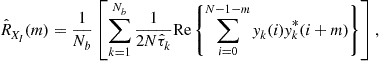 (11.53)
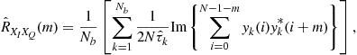 (11.54)
where ![]() is the number of data bursts and
is the number of data bursts and ![]() is the estimated value of the texture in the kth burst
is the estimated value of the texture in the kth burst ![]() where
where ![]() .
.
Figure 11.22 shows two plots of the real and the imaginary parts of the speckle autocorrelation function for 60 m and 3 m estimated with ![]() . This result provides a clear indication that for all resolutions and all polarizations, the speckle correlation time is about 10 ms and the behavior is oscillatory.
. This result provides a clear indication that for all resolutions and all polarizations, the speckle correlation time is about 10 ms and the behavior is oscillatory.
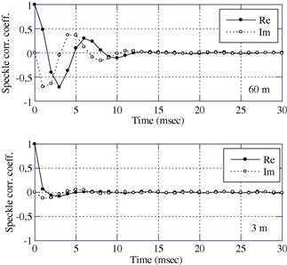
2.11.3.1.5 Estimation of the texture autocorrelation sequence
To check the validity of the hypothesis made on the correlation times of the two components, we can estimate the texture autocorrelation sequence with the formula:
 (11.55)
and the texture covariance as
 (11.56)
It is useful to observe that with a 50% of overlap, we can estimate the texture correlation and covariance every ![]() lags. In the figures we plot the texture correlation coefficient, that is
lags. In the figures we plot the texture correlation coefficient, that is ![]() , with N = 128.
, with N = 128.
Figures 11.23 and 11.24 show the texture correlation coefficient. At the same resolutions and without differences in the polarizations, the texture correlation time is on the order of seconds. Furthermore, the texture presents periodicities with a period of 8 s at a range resolution of 60 m and of 3 s at a range resolution of 30 m. The periodicity is particularly evident in the VV polarized data for the resolution of 60 m in all the analyzed files. These results show as well that, with increasing resolution, the texture correlation time decreases, but still in the order of few seconds and the periodicities tend to disappear, due to the strong contribution of the thermal noise (see Figure 11.24).

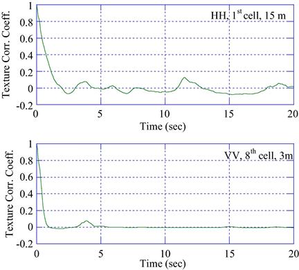
Figure 11.25 reports two examples of the average spectrogram in semi-logarithm scale calculated as
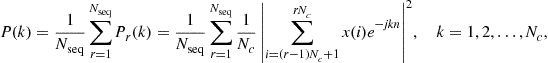 (11.57)
where ![]() is the number of sequences in which the received vector for each cell has been divided,
is the number of sequences in which the received vector for each cell has been divided, ![]() is the number of samples per sequence, k is the normalized frequency and
is the number of samples per sequence, k is the normalized frequency and ![]() is the kth sample of the periodogram of the rth sequence.
is the kth sample of the periodogram of the rth sequence.
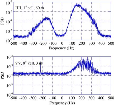
In these results, the periodogram shows, for all the polarizations, for all the range resolutions, a peak located around 150 Hz. Moreover, with a resolution of 60 m and 30 m, most of the analyzed cells show a bimodal spectrum, particularly evident in HH polarization, and then a second peak near −150 Hz; the power of the second peak is much lower than the power of the main one (see upper figure). From the resolution of 15 m, the IPIX radar seems to add a frequency interfering line in the spectrum at about −220 Hz (see lower figure). The line at 0 Hz is due to a residual of the continuous component. It is evident that, as resolution increases, the thermal noise effect becomes very important. In fact, the clutter-to noise ratio (CNR) decreases from ![]() for a resolution of 60 m and VV data to less than −5 dB for a resolution of 3 m and VH data. The CNR has been roughly estimated from the spectrum figures reading the value of the noise floor from each figure and calculating the clutter power as the difference between the overall disturbance power and the noise power. The values calculated for each cell is reported in the figure captions.
for a resolution of 60 m and VV data to less than −5 dB for a resolution of 3 m and VH data. The CNR has been roughly estimated from the spectrum figures reading the value of the noise floor from each figure and calculating the clutter power as the difference between the overall disturbance power and the noise power. The values calculated for each cell is reported in the figure captions.
2.11.3.1.6 Mean range texture autocovariance sequence
To conclude the correlation analysis, in order to highlight further differences due to the resolution, we can also calculate the average range autocovariance function of the texture given by
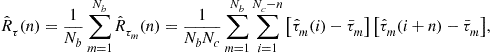 (11.58)
where ![]() is the estimate of the texture on the mth burst of the ith cell,
is the estimate of the texture on the mth burst of the ith cell, ![]() is the number of illuminated cells,
is the number of illuminated cells, ![]() is the number of bursts and
is the number of bursts and ![]() is the texture average value in the mth burst
is the texture average value in the mth burst ![]() .
.
Since at 30 m range resolution the illuminated zone is different, we compare here only the results found at 15 m, 9 m, and 3 m range resolutions.
Figure 11.26 shows the results obtained for VV and HH polarizations. From the figure it is evident that with a resolution of 3 m, it is possible to highlight and resolve shorter-range periodicities that are not visible in the other resolutions in all the polarizations.
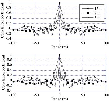
2.11.3.1.7 Sea clutter non-stationarity: Bragg scattering and long waves
So far we have considered the sea clutter process as a stationary stochastic process. Actually this is not true, and the behavior we have proved in the previous paragraphs holds true only “in average.” The non-stationarity of the sea clutter is due to its nature and some explanation is needed. Sea clutter is backscattered by a moving rough surface [59,60] characterized in terms of two fundamental types of waves. The first type is represented by capillary waves with wavelengths ![]() on the order of centimeters or less, the second by the longer gravity waves (sea or swell) with wavelengths ranging from a few hundred meters to less than a meter [59]. In deep water, for the capillary waves we have
on the order of centimeters or less, the second by the longer gravity waves (sea or swell) with wavelengths ranging from a few hundred meters to less than a meter [59]. In deep water, for the capillary waves we have ![]() , whereas for the gravity waves the wavelength is
, whereas for the gravity waves the wavelength is ![]() . Capillary waves are usually generated by turbulent gusts of near surface wind and their restoring force is the surface tension. On the contrary, swells are produced by stable winds and their restoring force is the gravity. Then, at any point on the surface the waves are complex summations of the locally generated wind waves and waves that have propagated in from other areas and different directions, resulting in a complex interaction [61].
. Capillary waves are usually generated by turbulent gusts of near surface wind and their restoring force is the surface tension. On the contrary, swells are produced by stable winds and their restoring force is the gravity. Then, at any point on the surface the waves are complex summations of the locally generated wind waves and waves that have propagated in from other areas and different directions, resulting in a complex interaction [61].
To take into account the presence of different scales of roughness in the sea surface, Wright [36] and Bass et al. [37] developed a two-scale model of the sea surface scattering in which the surface height is partitioned into a large-scale displacement and a small-scale displacement. For this model, it is assumed that over any patch of the surface that is large compared with small-scale lengths, but small compared with large-scale lengths, the scattering can be modeled as first-order Bragg scattering from the small-scale structure. Thus, the effect of the large-scale structure is to change the distance between the antenna and each point of the considered patch, by tilting the surface and advecting the small-scale structure both vertically and horizontally. The effect of large-scale surface tilt is to introduce an effective amplitude modulation of the small-scale scattering [62]. Conversely, the effect of the advection is to influence the frequency content of the overall scattering.
The Bragg scattering is based on the principle that the return signals from scatterers that are half a radar wavelength apart, measured along the line of sight from the radar, reinforce each other since they are in phase [59]. The Bragg resonant length is ![]() where
where ![]() is the wavelength of the radar signal and
is the wavelength of the radar signal and ![]() is the grazing angle. At microwave frequencies, the Bragg scattering is from capillary waves and
is the grazing angle. At microwave frequencies, the Bragg scattering is from capillary waves and ![]() , where g is the acceleration of free fall. As a consequence, the capillary waves approaching and receding in the radar line-of-sight direction give rise to two Bragg spectral lines located at
, where g is the acceleration of free fall. As a consequence, the capillary waves approaching and receding in the radar line-of-sight direction give rise to two Bragg spectral lines located at ![]() , at least in absence of other scattering phenomena and of the long waves. The magnitude of these lines depends on the azimuth look direction of the radar relative to the wind direction [41]. In a real scenario, the Bragg scatterers are advected by the orbital velocity of the intermediate waves (waves with wavelengths longer than the Bragg wavelength but shorter than the radar resolution cell) and of the long waves (waves with wavelengths longer than the radar resolution cell). The sum of the orbital velocities of the unresolved intermediate scale waves causes a spectral broadening around the Bragg lines. For many ocean conditions, these orbital motions broaden the Bragg lines by more than their separation, causing the lines to be unresolved, and generating only one Doppler peak. At X-band frequencies, this is generally the case [61,63]. Therefore, according to the Bragg theory, long waves that are resolved by high-resolution radars may be assumed to be constant over each illuminated cell. Consequently, their effect on the Doppler spectrum is to shift the Doppler peak according to the long wave orbital velocity. The orbital velocities are given by the simple harmonic motion
, at least in absence of other scattering phenomena and of the long waves. The magnitude of these lines depends on the azimuth look direction of the radar relative to the wind direction [41]. In a real scenario, the Bragg scatterers are advected by the orbital velocity of the intermediate waves (waves with wavelengths longer than the Bragg wavelength but shorter than the radar resolution cell) and of the long waves (waves with wavelengths longer than the radar resolution cell). The sum of the orbital velocities of the unresolved intermediate scale waves causes a spectral broadening around the Bragg lines. For many ocean conditions, these orbital motions broaden the Bragg lines by more than their separation, causing the lines to be unresolved, and generating only one Doppler peak. At X-band frequencies, this is generally the case [61,63]. Therefore, according to the Bragg theory, long waves that are resolved by high-resolution radars may be assumed to be constant over each illuminated cell. Consequently, their effect on the Doppler spectrum is to shift the Doppler peak according to the long wave orbital velocity. The orbital velocities are given by the simple harmonic motion ![]() , where f is the frequency of the long gravity wave of period T and H is its height from crest to trough. The contribution of the orbital velocity to the motion of the Bragg scatterers is the horizontal component, that is
, where f is the frequency of the long gravity wave of period T and H is its height from crest to trough. The contribution of the orbital velocity to the motion of the Bragg scatterers is the horizontal component, that is ![]() , where K is the wave number and x the spatial position [64]. The velocities of the scatterers in the nodes, crests and troughs of the waves are very different. Finally, an additional Doppler shift results from any surface currents present, including wind drift. A formula often used to represent this drift is
, where K is the wave number and x the spatial position [64]. The velocities of the scatterers in the nodes, crests and troughs of the waves are very different. Finally, an additional Doppler shift results from any surface currents present, including wind drift. A formula often used to represent this drift is ![]() , where
, where ![]() is the wind speed. Therefore, by considering the contribution of orbital velocity, current velocity
is the wind speed. Therefore, by considering the contribution of orbital velocity, current velocity ![]() and wind drift, we can calculate the time-varying instantaneous Doppler shift as (see the picture in Figure 11.27)
and wind drift, we can calculate the time-varying instantaneous Doppler shift as (see the picture in Figure 11.27) ![]() where
where ![]() is the intrinsic phase speed of the Bragg wave given by the wave dispersion relation. Due to the periodicity of
is the intrinsic phase speed of the Bragg wave given by the wave dispersion relation. Due to the periodicity of ![]() should be periodic as well. However, the Bragg scattering is not the only phenomenon determining the clutter return, particularly if breaking waves are present on the sea surface as clearly showed in [65,66] but it is generally dominant in down-wind VV data. Therefore, to see clearly the effect of the long waves on the sea return, we show here in detail some results of the analyses carried out on down-wind VV data [41].
should be periodic as well. However, the Bragg scattering is not the only phenomenon determining the clutter return, particularly if breaking waves are present on the sea surface as clearly showed in [65,66] but it is generally dominant in down-wind VV data. Therefore, to see clearly the effect of the long waves on the sea return, we show here in detail some results of the analyses carried out on down-wind VV data [41].

It is worth observing that in the modern statistical sea clutter literature, as already written, the small-scale structure scattering of the two-scale model corresponds to the speckle ([11,12,15,55]). The variations of the local power, due to the amplitude modulation of the speckle introduced by the tilting of the small-scale structure correspond to the texture. According to the compound-Gaussian model the texture and the speckle are two independent processes, the speckle is stationary and the texture amplitude modulates the speckle. However, as suggested by Haykin et al. [59], and as provided for by the two-scale model, the relationship between slowly and rapidly time-varying processes is much more complicated: the slowly varying swell motion does not only modulate the amplitude of the speckle, but also its mean frequency (Doppler centroid) and its bandwidth [41].
In this section of this tutorial, evidence of the modulating effect of long waves on speckle backscattering is verified through the analysis of experimental sea clutter data, collected in Dartmouth, Nova Scotia, at Osborne Head Gunnery Range (OHGR), with the IPIX radar.
The effect of the long waves on the overall scattering has been already considered in literature, but generally the analyses are theoretical or, when experimental, they consider only the average spectrum, that is, the spectrum calculated on the entire data set [27,28,61,67]. This kind of analysis can be exhaustive only when the radar resolution is low. In this case in fact, as explained in [67], the low-resolution radar performs a spatial averaging over many waves and the radar cannot see the different features of the waves passing through the resolution cell during the recording. Some evidence of the long wave and breaking wave amplitude and frequency modulation on the time-varying spectrum of real sea clutter is presented, for instance, in [59,64,68].
The sea clutter data shown here were collected at Osborne Head Gunnery Range (OHGR) with IPIX radar during the Dartmouth campaign. The characteristics and acquisition conditions of the analyzed file are summarized in Table 11.15. Data from all polarizations were processed, however, in this section we describe in more details the experimental results relative to the VV polarized data of the file Starea4 recorded on the 7 November 1993 at 11:23 pm. This dataset was recorded in conditions particularly apt to reveal the long wave modulating effects (that is our main interest here), both for the fully developed sea state and for the radar downwind direction. During the time the data was collected, the Canadian Forecast Service reported that the significant wave height was of 2.23 m with an average period of 8.3 s. The wind was blowing with a speed of 4–15 km/h since 8 pm of 6 November, coming to a relative calm state (1–3 in the Beaufort scale) after it has been blowing with strong velocity (35–45 km/h) for the previous 24 h. The wind direction was ![]() from the North since 10 am, and the azimuth angle was fixed at
from the North since 10 am, and the azimuth angle was fixed at ![]() from the North (
from the North (![]() of difference, approximately down-wind). Due to these conditions in the VV data the Bragg scattering was dominant.
of difference, approximately down-wind). Due to these conditions in the VV data the Bragg scattering was dominant.
A statistical analysis performed on these data as described in the previous paragraphs, showed that this clutter is GK distributed [41].
As already stated, the selection of the vertical polarization is justified because Bragg scattering was dominant (in the recording conditions of file Starea4) and the effect of long-waves should be clear and evident. Figure 11.28 shows the time evolution of the texture, estimated as ![]() , where
, where ![]() , is the nth sample of the complex envelope of the data,
, is the nth sample of the complex envelope of the data, ![]() is the number of bursts in which the entire sequence of the range cell data has been divided,
is the number of bursts in which the entire sequence of the range cell data has been divided, ![]() is the number of samples in the lth burst (adjacent bursts have an overlap of 50%). It has been assumed (and verified) that the texture is constant within each short burst of 0.128 s. The almost-periodic behavior of the texture is evident for both polarizations.
is the number of samples in the lth burst (adjacent bursts have an overlap of 50%). It has been assumed (and verified) that the texture is constant within each short burst of 0.128 s. The almost-periodic behavior of the texture is evident for both polarizations.

Figure 11.28 HH and VV polarized backscattering mean texture, versus the observation time interval. Dataset: Starea4 of November 7, range cell 3.
In the frequency domain, the presence of periodicity in the power, and then of an amplitude modulating effect of the swells, is evidenced by the time-varying spectrogram in Figure 11.29a, where the spectrogram is plotted in a linear colormap from blue to red in the frequency range −200 to 200 Hz, where we have most of the sea clutter contribution (the variability of the sea spectrum was also visible in Figure 11.9. The plots in this figure were obtained by computing the FFT over a sliding window of 512 samples (0.512 s), weighed by a Hanning window, and with an overlap of 50%. The 512-points FFT ![]() provides the spectrogram in the frequency range −500 to 500 Hz. It is apparent that the mean texture and spectrogram illustrate a common periodic trend with a period of about 10 s that is comparable with those of the swells after projection on the radar line of sight. However, the effect of long waves is not limited to an amplitude modulation. It involves also a periodic change in the shape, bandwidth and maximum of the time-varying spectrum. This aspect is better revealed by the normalized spectrogram reported in Figure 11.29b (the spectrogram in Figure 11.29a was not normalized). The entire sequence of data has been again divided into
provides the spectrogram in the frequency range −500 to 500 Hz. It is apparent that the mean texture and spectrogram illustrate a common periodic trend with a period of about 10 s that is comparable with those of the swells after projection on the radar line of sight. However, the effect of long waves is not limited to an amplitude modulation. It involves also a periodic change in the shape, bandwidth and maximum of the time-varying spectrum. This aspect is better revealed by the normalized spectrogram reported in Figure 11.29b (the spectrogram in Figure 11.29a was not normalized). The entire sequence of data has been again divided into ![]() bursts of
bursts of ![]() samples each, with an overlap between adjacent bursts of 50%. Individual spectra have been calculated using a 512-point FFT and Hanning windowing, and then normalized with respect to the local clutter power. The non-stationarity of the sea clutter related to the periodic spectral variations is evident. These variations correspond to the changes of the frequency extent and of the Doppler peak due to the frequency modulation induced by the long waves on the Bragg-wave scattering.
samples each, with an overlap between adjacent bursts of 50%. Individual spectra have been calculated using a 512-point FFT and Hanning windowing, and then normalized with respect to the local clutter power. The non-stationarity of the sea clutter related to the periodic spectral variations is evident. These variations correspond to the changes of the frequency extent and of the Doppler peak due to the frequency modulation induced by the long waves on the Bragg-wave scattering.
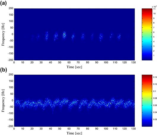
In order to measure the temporal variation of the backscattered Doppler spectra, we can measure the Doppler centroid of the clutter spectrum and the rms (root mean square) bandwidth, defined respectively as
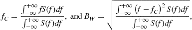 (11.59)
where f is the frequency and ![]() is the clutter PSD. The behavior of the Doppler centroid is investigated instead of that of the PSD peak because it is generally more representative of the short-time spectrum change, especially in the case of non-symmetric spectral shape. To estimate the time-varying centroid and bandwidth we can calculate:
is the clutter PSD. The behavior of the Doppler centroid is investigated instead of that of the PSD peak because it is generally more representative of the short-time spectrum change, especially in the case of non-symmetric spectral shape. To estimate the time-varying centroid and bandwidth we can calculate:
 (11.60)
where ![]() is the digital frequency,
is the digital frequency, ![]() is the periodogram of the lth data burst (composed of 512 samples) corresponding to f (n), computed on
is the periodogram of the lth data burst (composed of 512 samples) corresponding to f (n), computed on ![]() points and
points and ![]() .
.
Figure 11.30 shows the time evolution of the texture (on arbitrary scale and units, for ease of representation), Doppler centroid, and bandwidth, obtained by processing the data from the third range cell. They exhibit a common periodic trend with their own reciprocal delay. The Doppler centroid varies between −50 Hz and 5 Hz, the bandwidth between 25 Hz and 225 Hz. We observe that the maxima in the texture values are coincident with the minima of the bandwidth and vice versa. The spectral enlargement could be due to the modulation induced by the long waves or the presence of thermal noise. The effect of this noise in the spectral and temporal features of the received echo may be quite different depending on the clutter-to-noise power ratio (CNR). In the analyzed file, the CNR ranges from about 80 dB when the texture is maximum to about −5 dB when the texture is minimum [41]. In the latter case, the contribution of the noise to the echo is strong. The Doppler centroid and the bandwidth follow the texture behavior but with small delays of 2–3 s and 5 s respectively, i.e., about 1/4 and 1/2 of the swell period.
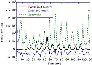
Figure 11.30 Time evolution of VV polarized backscattering mean texture, Doppler centroid and bandwidth. Dataset: Starea4 of November 7, range cell 3, VV polarization.
In order to quantify the relationship between texture, centroid and bandwidth, we can use their cross-covariance functions (CCF). The CCF between the time-varying texture and the Doppler centroid signals can be calculated as
 (11.61)
and for texture and bandwidth:
 (11.62)
where, ![]() and
and ![]() are the estimated texture, Doppler centroid and bandwidth, and
are the estimated texture, Doppler centroid and bandwidth, and
 (11.63)
are their respective sample means. Figure 11.31a and b shows the plots of ![]() and
and ![]() , respectively. They show a behavior very similar to the cross-covariance functions between two truncated sinusoids with a common period of about 10 s separated by a lag of about 2.5 s and 5 s, respectively.
, respectively. They show a behavior very similar to the cross-covariance functions between two truncated sinusoids with a common period of about 10 s separated by a lag of about 2.5 s and 5 s, respectively.

Figure 11.31 (a, b) Cross-covariance between mean texture and Doppler centroid, and between mean texture and bandwidth. Dataset: Starea4 of November 7, range cell 3, VV polarization.
In order to retrieve the actual frequency values of the common sinusoidal components, it is useful to calculated the absolute value of the mutual PSDs, i.e., the absolute value of the Fourier transform of ![]() and
and ![]() . The results of this calculation are shown in Figure 11.32a and b. The information on the frequency “similarity” of texture and centroid provided by these mutual PSDs is analogous to that contained in the modulation transfer function (MTF) known to the geophysics community (see, for instance, [62] and references therein). The peaks in the mutual PSD correspond to the frequencies common to the two analyzed signals. This means, for instance, that the frequency component at
. The results of this calculation are shown in Figure 11.32a and b. The information on the frequency “similarity” of texture and centroid provided by these mutual PSDs is analogous to that contained in the modulation transfer function (MTF) known to the geophysics community (see, for instance, [62] and references therein). The peaks in the mutual PSD correspond to the frequencies common to the two analyzed signals. This means, for instance, that the frequency component at ![]() is present in both texture and Doppler centroid signals and in both texture and bandwidth signals. This fact is confirmed by the normalized Fourier spectrum of texture, Doppler centroid and bandwidth (calculated after sample mean removal). The curves are in Figure 11.33a–c. They confirm the hypothesis of a near line-shape Doppler spectrum with components located in correspondence with the long wave frequency
is present in both texture and Doppler centroid signals and in both texture and bandwidth signals. This fact is confirmed by the normalized Fourier spectrum of texture, Doppler centroid and bandwidth (calculated after sample mean removal). The curves are in Figure 11.33a–c. They confirm the hypothesis of a near line-shape Doppler spectrum with components located in correspondence with the long wave frequency ![]() . Moreover, secondary components are present close to
. Moreover, secondary components are present close to ![]() and, especially for texture and bandwidth spectra, at
and, especially for texture and bandwidth spectra, at ![]() . These results suggest that, at least when Bragg scattering is dominant, the long waves modulate the speckle scattering in amplitude, causing the variation of the local power, and in frequency, causing a periodic variation of the spectrum centroid and bandwidth.
. These results suggest that, at least when Bragg scattering is dominant, the long waves modulate the speckle scattering in amplitude, causing the variation of the local power, and in frequency, causing a periodic variation of the spectrum centroid and bandwidth.

2.11.3.1.8 AR model
As apparent, there are two goals related to clutter modeling. The first is to provide further insight into the physical and electromagnetic factors that play a role in forming the clutter signal. The second is to produce a mathematical model, physically grounded, with which the clutter signal can be generated and processed to test detection algorithms. In this section, we suggest the use of AR modeling to describe the physical phenomenon of the long wave modulation analyzed in the previous section. As known, the autoregressive models can fit both Gaussian and non-Gaussian (as in our case) processes [70, Chapter 4].
The model’s ability to describe a physical phenomenon is not the main constraint, its mathematical tractability is also very important. In [41] the authors found that an AR model of the third order, AR(3), allows these constrictions. As regards the tractability, the AR(3) model is defined by seven real parameters, the complex value of its three poles and the final prediction error. Moreover, an AR process can be simply generated by properly filtering white noise.
The normalized periodogram of the data was obtained by averaging the individual normalized Fourier spectra related to single sliding bursts. The entire sequence of data has been divided into ![]() bursts of
bursts of ![]() samples each, with an overlap between adjacent bursts of 50%. Next, individual Fourier spectra were calculated using a 512-point FFT and a Hanning window and then normalized with respect to the local clutter power. As regards the AR spectrum, it was obtained by processing all the range cell samples via Yule-Walker’s method [71]. In Figure 11.34 we report some results for an AR(3) process. It seems that the AR(3) can describe the basic shape features such as Doppler centroid and bandwidth.
samples each, with an overlap between adjacent bursts of 50%. Next, individual Fourier spectra were calculated using a 512-point FFT and a Hanning window and then normalized with respect to the local clutter power. As regards the AR spectrum, it was obtained by processing all the range cell samples via Yule-Walker’s method [71]. In Figure 11.34 we report some results for an AR(3) process. It seems that the AR(3) can describe the basic shape features such as Doppler centroid and bandwidth.
This is confirmed by Figure 11.35a and b that represent the time evolution of these quantities, estimated both by the spectrogram and by the AR method. In particular, the estimated AR centroid is given by

Figure 11.35 (a,b) Time evolution of the Doppler centroid and bandwidth, obtained from the Fourier and AR(3) estimated spectra. Dataset: Starea4 of November 7, range cell 3, VV polarization.
 (11.64)
while the estimated AR bandwidth is
 (11.65)
where ![]() is the digital frequency,
is the digital frequency, ![]() is the AR spectrum computed by processing the 512 samples of the lth data burst, via Yule-Walker’s method on
is the AR spectrum computed by processing the 512 samples of the lth data burst, via Yule-Walker’s method on ![]() points, and
points, and ![]() . Figure 11.36a and b shows the Fourier spectrum of the AR(3)-centroid and AR(3)-bandwidth. AR centroid and AR bandwidth still preserve the spectral components of the corresponding quantities obtained by the Fourier analysis. Also, the time delay with respect to texture is preserved, as shown by the cross-covariance (Figure 11.37a and b). Therefore, this analysis suggests that AR(3) model is able to model the basic effects of long waves modulation on the capillary backscattering.
. Figure 11.36a and b shows the Fourier spectrum of the AR(3)-centroid and AR(3)-bandwidth. AR centroid and AR bandwidth still preserve the spectral components of the corresponding quantities obtained by the Fourier analysis. Also, the time delay with respect to texture is preserved, as shown by the cross-covariance (Figure 11.37a and b). Therefore, this analysis suggests that AR(3) model is able to model the basic effects of long waves modulation on the capillary backscattering.

Figure 11.36 (a,b) Normalized Fourier spectrum of the AR(3) Doppler centroid, and AR(3) bandwidth. Dataset: Starea4 of November 7, range cell 3.
Figure 11.37 (a,b) Cross-covariance between mean texture and the AR(3) Doppler centroid, and between mean texture and the AR(3) bandwidth. Dataset: Starea4 of November 7, range cell 3.
It is also of interest to investigate how its parameters vary. Figures 11.36a–c show the time evolution of the two dominant AR poles and final prediction error, together with texture. The elements of correlation are evident. The dominant pole, with almost constant unitary modulus, has an instantaneous frequency that varies with the same period of the texture. Also, the second pole follows the same periodic trend, being almost constant when the signal is strongly reflected by the crest of a wave and noisy otherwise. The third pole is dominated by noise, while the final prediction error follows the texture trend.
From the results shown in the previous pages, it is apparent that there is not a unique optimum amplitude and spectral model for the sea clutter in all the resolutions. The statistical parameters change with time, range resolution, polarization, sea conditions. Generally the compound-Gaussian model provides a good fitting to the data but it shows some limits at the very high resolutions particularly for HH data, which are almost always spikier than VV data. Moreover, the sea clutter cannot be considered stationary on long periods of time. As particularly evident in X-band and VV pol, the long waves modulate the sea scattering in amplitude and frequency, determining the temporal and spatial periodical changes of the texture and of the bandwidth and Doppler centroid of the speckle spectrum.
2.11.3.2 Land clutter analysis: farmland area
The results of the analysis of ground clutter, reported in this section, mainly relate to the data recorded with the MIT Lincoln Laboratory Phase One radar [29,32].
The Phase One radar could operate in any one of five different radar bands (VHF, UHF, L-, S-, and X-bands). The results of this section are for ground clutter data recorded at X-band. Results in all bands are given in [32]. The overall radar system block diagram description can be found in [29].
The radar maintained coherence and stability sufficient for 60 dB, two-pulse-canceller clutter attenuation in post-processing and also had uncoded pulsed waveforms, with two pulse lengths available in each band to provide high and low range resolutions. Polarization was selectable as vertical or horizontal, with transmit and receive antennas always co-polarized, i.e., the cross-polarized component in the radar return signal could not be received. Frequency, polarization, and pulse length as well as spatial extent in range and azimuth of the recording window, number of pulses, and pulse-repetition rate were selectable by computer console for each recorded clutter experiment.
The analyzed clutter data files described here were recorded at X-band at Wolseley, Saskatchewan, located on the Canadian prairie at a latitude of ![]() N and a longitude of 103.150W. The illuminated area was covered by agricultural crops (83%), deciduous trees (11%), lakes (4%), and rural farm buildings (2%). The terrain was a sequence of gentle slopes (
N and a longitude of 103.150W. The illuminated area was covered by agricultural crops (83%), deciduous trees (11%), lakes (4%), and rural farm buildings (2%). The terrain was a sequence of gentle slopes (![]() ) with a relief of 25–150 ft.
) with a relief of 25–150 ft.
The analyzed X-band (9.2 GHz) data are divided in two different sets. In the first one (N007001.35) the polarization is HH, in the second one (N007001.34) it is VV. Each set contains four range intervals recorded in scan mode, and each range interval contains 316 range cells. The scan velocity was ![]() /s, i.e., about 2 beams/s. The emitted pulse repetition frequency (PRF) was 500 Hz, but only 1 out of 2 pulse returns was recorded. The pulses were further coherently integrated in groups of 16, so the effective PRF of the data from this experiment is 15.625 Hz. The data were stored in a 316
/s, i.e., about 2 beams/s. The emitted pulse repetition frequency (PRF) was 500 Hz, but only 1 out of 2 pulse returns was recorded. The pulses were further coherently integrated in groups of 16, so the effective PRF of the data from this experiment is 15.625 Hz. The data were stored in a 316 ![]() 703 matrix, each row for a fixed range, each column for a fixed azimuth. For each integrated pulse, 316 range samples are provided at 10 MHz sampling rate. The data were collected one range interval after another in “windshield-wiper” mode (see [29] for more details).
703 matrix, each row for a fixed range, each column for a fixed azimuth. For each integrated pulse, 316 range samples are provided at 10 MHz sampling rate. The data were collected one range interval after another in “windshield-wiper” mode (see [29] for more details).
The radar depression angle decreased from about ![]() to
to ![]() across the first range interval, and further decreased to
across the first range interval, and further decreased to ![]() in the second interval, to
in the second interval, to ![]() in the third interval and to
in the third interval and to ![]() in the fourth range interval. The azimuth beamwidth of the antenna was 0.018 rad at HH polarization and 0.019 rad about 10 (i.e., at VV polarization). The nominal azimuth sampling interval was
in the fourth range interval. The azimuth beamwidth of the antenna was 0.018 rad at HH polarization and 0.019 rad about 10 (i.e., at VV polarization). The nominal azimuth sampling interval was ![]() /pulse; thus for each range cell the radar recorded seven to eight azimuth samples. The range resolution was 15 m (i.e., pulse length
/pulse; thus for each range cell the radar recorded seven to eight azimuth samples. The range resolution was 15 m (i.e., pulse length ![]() 100 ns, which matches the 10 MHz sampling rate). The return from each pulse was provided in I and Q format calibrated in units of radar cross section [32]. The analysis was performed on the data after normalizing them with respect to the square root of the cell area. This normalization is helpful in comparing results for statistical populations extended in range, as these Wolseley data. The normalization makes the amplitude values of clutter returns independent of the distance.
100 ns, which matches the 10 MHz sampling rate). The return from each pulse was provided in I and Q format calibrated in units of radar cross section [32]. The analysis was performed on the data after normalizing them with respect to the square root of the cell area. This normalization is helpful in comparing results for statistical populations extended in range, as these Wolseley data. The normalization makes the amplitude values of clutter returns independent of the distance.
In Figure 11.39a the 2D clutter map relative to the first range interval of the VV polarized data is reported. The data are plotted in logarithmic scale to span the grey-scale code (0–255). The black areas of the image indicate regions of high radar reflectivity, usually from discrete vertical clutter sources, such as buildings, fence lines, trees, and bushes, aligned along roads and field borders; the white areas indicate regions of relatively low reflectivity, such as field surfaces. On the x-axis the 316 range samples are reported from 1 km to 5.7 km, whereas on the y-axis the 703 azimuth samples are from ![]() to
to ![]() .
.
Figure 11.39b shows the same data as Figure 11.39a, but in a 3D format to highlight the presence of spikes, well evident in this range interval. Wolseley is a generally open farmland site of low relief. At open farmland sites like Wolseley, spatial clutter statistics are dominated by spatially localized, fixed, discrete scatterers that comprise all the vertical objects that occur on the landscape. These include the isolated trees and small clusters of trees; agricultural field boundaries and the vertical objects along them such as fences and higher uncultivated vegetation (tall grass, shrubs); roads and the vertical objects along them such as utility poles and wires; banks of streams and creeks; complexes of farm buildings and farm machinery; other cultural artifacts such as water towers and radio towers; and, also, locally high points in the microtopography itself. Such discrete objects cause strong spikes of clutter distributed randomly over the agricultural field surfaces, which themselves constitute a relatively weak, area-extensive, backscattering medium. These spikes of clutter are observed in Figure 11.38b, where the curvilinear patterns indicate field and road boundaries on a predominantly north-south, east-west grid. Such spikes are of extremely wide variation in amplitude and result in long tails in empirical clutter spatial amplitude distribution applicable to such terrain.

Figure 11.38 (a–c) AR(3) pole frequencies and final prediction error, compared with the normalized texture.
The first step of the analysis done on these data was the check of the Gaussianity of the I and Q components. To this purpose the histograms of the I and Q components have been drawn, for each range interval and for each polarization (VV and HH). The histogram has been compared with the Gaussian PDF having the same mean and variance of the data. The dc offset of each channel has been estimated from each of the four range intervals of 316 ![]() 703 = 222,148 samples, and then subtracted from the data. This analysis, performed on each range interval, has shown that I and Q PDFs deviate considerably from Gaussianity; the clutter amplitude is therefore not Rayleigh distributed. This deviation is well evident in Figure 11.40, where the histogram of the I component for the fourth range interval (VV polarization) is compared with the Gaussian PDF having the same variance and zero-mean.
703 = 222,148 samples, and then subtracted from the data. This analysis, performed on each range interval, has shown that I and Q PDFs deviate considerably from Gaussianity; the clutter amplitude is therefore not Rayleigh distributed. This deviation is well evident in Figure 11.40, where the histogram of the I component for the fourth range interval (VV polarization) is compared with the Gaussian PDF having the same variance and zero-mean.

These results were confirmed by estimating the skewnessand kurtosis,defined, respectively, as
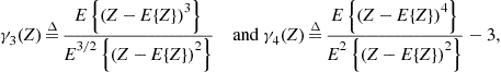 (11.66)
where E{Z} is the mean value of the random variable Z. The skewness characterizes the degree of asymmetry of a distribution around its mean value. A positive value of skewness corresponds to a distribution with an asymmetric tail extending on the right of the mean. A negative value of the skewness corresponds to a distribution with an asymmetric tail extending on the left. The kurtosis measures the relative peakedness or flatness of a distribution. For a Gaussian PDF these two parameters are identically zero, so they are a measure of the deviation from Gaussianity. The estimates of the skewness and kurtosis from two range intervals are reported in Table 11.16.

The study of the data has been completed performing a statistical analysis similar to that performed on the sea clutter data, comparing the histogram with some known distributions. The results show that the data seem to fit best the Weibull distribution for the first and second range intervals, while for the third and fourth range intervals the data show a behavior that is intermediate between Weibull and log-normal [29]. The results of histogram analysis for the fourth range cell are reported in Figure 11.41 on a log-scale.
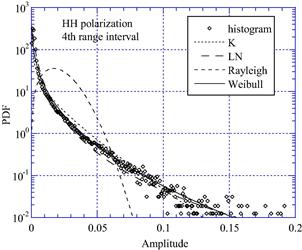
The same results were obtained for the VV data of the same site.
2.11.3.2.1 Modified Kolmogorov-Smirnoff statistical test
The statistical analysis of data amplitude was concluded by applying a statistical hypothesis test as for the sea clutter data. The KS goodness-of-fit test has been largely used to determine which distribution (Rayleigh, log-normal, Weibull, or K in our case) best fits the data. Unfortunately, as already said for sea clutter, in some cases it is not useful, because it places an equal importance on all regions in the probability space. In practical radar applications a good fit is important in the tail regions of the PDFs. The tails, in fact, contain the strong values (i.e., the spikes) that, considered as target returns by a detector, can increase the FAR. Since good fitting in the tails is mandatory for correct design of CFAR processors, especially when low ![]() values are required, the KS test is of limited use for clutter data (as recognized also in [32]). To overcome this problem we can use a modified Kolmogorov-Smirnoff (MKS) goodness-of-fit test [29].
values are required, the KS test is of limited use for clutter data (as recognized also in [32]). To overcome this problem we can use a modified Kolmogorov-Smirnoff (MKS) goodness-of-fit test [29].
The idea is simple: apply the standard KS test by taking into account only the tail regions, i.e., by considering only the data above a given threshold AMKS and the modified theoretical PDFs ![]() where
where ![]() is the unit step function. The standard two-sample KS test verifies whether the recorded data are distributed in accordance with a hypothetical PDF, as already said for the sea clutter data. If the probability of type I is very low, for instance <1%, then this hypothesis should be rejected [72]. By applying the standard two-sample test, which considers the entire definition range of the random variable Z under investigation, the obtained probability of Type I error
is the unit step function. The standard two-sample KS test verifies whether the recorded data are distributed in accordance with a hypothetical PDF, as already said for the sea clutter data. If the probability of type I is very low, for instance <1%, then this hypothesis should be rejected [72]. By applying the standard two-sample test, which considers the entire definition range of the random variable Z under investigation, the obtained probability of Type I error ![]() is always <1%, for all the distributions (Rayleigh, log-normal, Weibull, and K); thus, in the classical formulation, the KS test is not useful with these data. This is due to the differences exhibited by the distributions in the region of low values of Z. On the contrary, if we apply the MKS test setting the threshold AMKS in the region (0.01, 0.03), where the distributions are very similar (except for the Rayleigh), the result for the probability of type I is always 100%. This means that, in this central region, the KS test cannot distinguish between the different proposed models. But, as written above, we are mainly interested in the tails of the distribution, so we can applied the MKS test with, for instance,
is always <1%, for all the distributions (Rayleigh, log-normal, Weibull, and K); thus, in the classical formulation, the KS test is not useful with these data. This is due to the differences exhibited by the distributions in the region of low values of Z. On the contrary, if we apply the MKS test setting the threshold AMKS in the region (0.01, 0.03), where the distributions are very similar (except for the Rayleigh), the result for the probability of type I is always 100%. This means that, in this central region, the KS test cannot distinguish between the different proposed models. But, as written above, we are mainly interested in the tails of the distribution, so we can applied the MKS test with, for instance, ![]() . In this way we leave out of the analysis the central region of the PDF, corresponding to high values of
. In this way we leave out of the analysis the central region of the PDF, corresponding to high values of ![]() (say,
(say, ![]() . The results are reported in Table 11.17.
. The results are reported in Table 11.17.

Generally, the value of probability of error of type I, ![]() , for Weibull PDF is higher than for the other PDFs, so the good fit of these ground clutter data to the Weibull model is confirmed.
, for Weibull PDF is higher than for the other PDFs, so the good fit of these ground clutter data to the Weibull model is confirmed.
2.11.3.2.2 Windblown trees data
The same analysis of farmland data was performed in [73] on a different Phase One X-band file, namely H067032.2, for which the data were measured from range cells containing windblown trees in contrast to open farmland. The clutter data shown here were recorded at Katahdin Hill site by Lincoln Laboratory personnel on 17 April 1985 [32]. The analyzed data set contains 30,720 samples per range cell, of HH-polarization, with pulse repetition frequency (PRF) equal to 500 Hz, and therefore pulse repetition interval (PRI) of T = 1/PRF = 2 ms. The return from each pulse is provided in in-phase and quadrature format. Data were recorded from 76 contiguous range gates utilizing the Phase One X-band stationary antenna in a fixed azimuth position (![]() ). These 76 range cells were located from 2.0 km to 3.1 km. The radar depression angle was about
). These 76 range cells were located from 2.0 km to 3.1 km. The radar depression angle was about ![]() and the azimuth beamwidth of the antenna was 0.018 rad. The radar range resolution was 15 m. The illuminated area was tree covered, primarily with mixed deciduous trees, but also with occasional pine and cedar. At the time of the experiments, the deciduous trees did not yet have their leaves. During this experiment the wind was quite strong: 15–20 knots. Details about how the data were collected can be found in [32]. The 3D power map of the clutter is shown in Figure 11.42.
and the azimuth beamwidth of the antenna was 0.018 rad. The radar range resolution was 15 m. The illuminated area was tree covered, primarily with mixed deciduous trees, but also with occasional pine and cedar. At the time of the experiments, the deciduous trees did not yet have their leaves. During this experiment the wind was quite strong: 15–20 knots. Details about how the data were collected can be found in [32]. The 3D power map of the clutter is shown in Figure 11.42.
In this figure the presence of two regions, with different power values, is evident. The curves representing the received power versus range exhibit a stepwise behavior. This is due to the transition between agricultural fields/wetland (first region) and windblown trees (second region). In our analysis here we consider only single range cells from the second region. In Figure 11.43 the histogram of the data relative only to the range cells 34–36 is compared with the Rayleigh PDF with the same variance.

The results obtained for the open farmland data (two data files N007001.34 and N007001.35) are very different from these windblown trees data. This is partly due to the different land covers of the illuminated areas, but also importantly, partly due to the forest data embodying temporal variations, not spatial. The area relative to the H067032.3 data file was homogeneously tree covered, primarily with mixed deciduous trees and with occasional pine and cedar. In the other two analyzed data files, the returns came from a large spatial population of fixed discrete sources on open farmland. This heterogeneity introduces a considerable spread in the distributions as already noted in [32]. The differences are also due to the way of recording the data: the windblown tree data are temporal statistics (variations in time on a given range cell, or on few cells) recorded with fixed antenna; the Wolseley farmland data are spatial statistics, recorded with a scanning antenna on many range cells.
2.11.3.2.3 The experimentally-measured Doppler spectrum of ground clutter
The Katahdin Hill data are particularly interesting for the shape of the PSD.
A suitable analytic expression of the PSD of ground clutter, ![]() , back-scattered from regions containing windblown vegetation [32], is
, back-scattered from regions containing windblown vegetation [32], is
![]() (11.67)
(11.67)
where f is the Doppler frequency in Hz, r is the ratio of dc power to ac power in the spectrum, ![]() is the Dirac delta function which represents the shape of the dc component in the spectrum and
is the Dirac delta function which represents the shape of the dc component in the spectrum and ![]() represents the shape of the ac component of the spectrum, normalized such that
represents the shape of the ac component of the spectrum, normalized such that ![]() . A phenomenological interpretation of this spectral shape was proposed in [74], where the exponential spectrum is obtained as the limit power spectrum in the presence of a random number of fluctuation scales in the Doppler components of windblown vegetation. From the detailed analyses of the MIT-LL measurements, it is apparent that the value of the dc/ac ratio r in Eq. (11.67) is strongly dependent on both wind speed and radar frequency and generally follows the empirically-derived analytical expression
. A phenomenological interpretation of this spectral shape was proposed in [74], where the exponential spectrum is obtained as the limit power spectrum in the presence of a random number of fluctuation scales in the Doppler components of windblown vegetation. From the detailed analyses of the MIT-LL measurements, it is apparent that the value of the dc/ac ratio r in Eq. (11.67) is strongly dependent on both wind speed and radar frequency and generally follows the empirically-derived analytical expression ![]() where w is wind speed in miles/hour, and
where w is wind speed in miles/hour, and ![]() is the radar carrier frequency in MHz. As described in [32], the MIT-LL measurements show a good fit to the model of Eq. (11.67) when the ac component of the spectrum is characterized by the two-sided exponential spectral shape
is the radar carrier frequency in MHz. As described in [32], the MIT-LL measurements show a good fit to the model of Eq. (11.67) when the ac component of the spectrum is characterized by the two-sided exponential spectral shape
![]() (11.68)
(11.68)
where ![]() is the radar transmission wavelength and
is the radar transmission wavelength and ![]() is the exponential shape parameter. The value of
is the exponential shape parameter. The value of ![]() is a function of the wind conditions such that the spectral width increases with increasing wind speed (see Table 11.18); however,
is a function of the wind conditions such that the spectral width increases with increasing wind speed (see Table 11.18); however, ![]() is largely independent of radar carrier frequency over the range from VHF to X-Band. An algebraic expression for
is largely independent of radar carrier frequency over the range from VHF to X-Band. An algebraic expression for ![]() that incorporates the linear dependency of spectral width on the logarithm of the wind speed w (mph) as observed in the data is
that incorporates the linear dependency of spectral width on the logarithm of the wind speed w (mph) as observed in the data is ![]() .
.
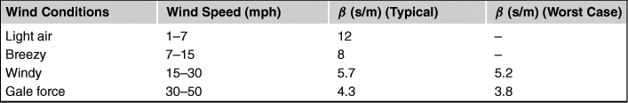
The described equations and Table 11.18 constitute a simple but complete model for characterizing the complex physical phenomenon of windblown clutter spectra over spectral dynamic ranges reaching 60–80 dB below zero-Doppler peaks, applicable over the range from VHF to X-band [32].
The Gaussian model for the windblown clutter spectrum, which was supported by early measurements with very limited dynamic range, is given by
![]() (11.69)
(11.69)
where ![]() is the standard deviation of the Gaussian spectrum. The exponential model has wider tails than the Gaussian model. For use with somewhat increased dynamic range, the other alternative popular spectral shape function
is the standard deviation of the Gaussian spectrum. The exponential model has wider tails than the Gaussian model. For use with somewhat increased dynamic range, the other alternative popular spectral shape function ![]() has been the power-law spectrum, which is characterized by two parameters, the shape parameter n, and the break-point Doppler frequency
has been the power-law spectrum, which is characterized by two parameters, the shape parameter n, and the break-point Doppler frequency ![]() that determines where the shape function is 3 dB below its peak zero-Doppler level:
that determines where the shape function is 3 dB below its peak zero-Doppler level:
![]() (11.70)
(11.70)
The MIT-LL measurements of much increased dynamic range clearly indicate that clutter spectral shapes are indeed wider than Gaussian; but that observed rates of decay modeled as power-law at upper levels of spectral power do not continue as power-law to lower levels of spectral power, but fall off much faster at the lower levels. The tails of the exponential model show an intermediate rate of decay—between the fast decay of the Gaussian model and the slow decay of the power-law model—that yields a good fit to the measured data.
For analyzing the PSD of windblown tree clutter, many data from various windblown-tree range cells were processed. Here we report only the results from range cell #35 (second region) as representative of results achieved by processing other range cells in the same region. The PSD has been first estimated non-parametrically, by using the modified periodogram method (Welch method) with the four-sample Blackman-Harris window [73]:
 (11.71)
with coefficients ![]() , and
, and ![]() . The set of 30,720 data samples has been divided in L = 15 subsets
. The set of 30,720 data samples has been divided in L = 15 subsets ![]() , with
, with ![]() , of N = 2048 samples each and then the windowed periodogram calculated from each subset as follows
, of N = 2048 samples each and then the windowed periodogram calculated from each subset as follows
 (11.72)
where ![]() , for
, for ![]() , and
, and ![]() is the nth complex sample relative to the kth subset. To obtain the final spectrum estimate, the K estimates are averaged as
is the nth complex sample relative to the kth subset. To obtain the final spectrum estimate, the K estimates are averaged as ![]() . Finally, the estimate is normalized such that the area is unity, i.e., divided by the estimate of the total disturbance power
. Finally, the estimate is normalized such that the area is unity, i.e., divided by the estimate of the total disturbance power ![]() . The disturbance power is estimated to be
. The disturbance power is estimated to be ![]() . The resulting curve is shown in Figure 11.44, labeled as “WP,” which stands for weighted periodogram. Note that the PSD is plotted from −250 Hz to 250 Hz because the PRF is 500 Hz. It is quite evident in these figures that, for
. The resulting curve is shown in Figure 11.44, labeled as “WP,” which stands for weighted periodogram. Note that the PSD is plotted from −250 Hz to 250 Hz because the PRF is 500 Hz. It is quite evident in these figures that, for ![]() , thermal noise predominates over clutter; thus we fit the clutter PSD only over the frequency range
, thermal noise predominates over clutter; thus we fit the clutter PSD only over the frequency range ![]() . In [73] the authors used the frequency bins in the range
. In [73] the authors used the frequency bins in the range ![]() to estimate the clutter-to-noise power ratio (CNR), which is obtained by solving the equation
to estimate the clutter-to-noise power ratio (CNR), which is obtained by solving the equation ![]() with respect to CNR, where
with respect to CNR, where ![]() is the thermal noise power,
is the thermal noise power, ![]() denotes the normalized PSD estimate and the sum is over all i’s such that
denotes the normalized PSD estimate and the sum is over all i’s such that ![]() . For the 35th range cell it results that
. For the 35th range cell it results that ![]() .
.

To estimate the clutter PSD parameters, nonlinear least squares (NLLS) method [15] has been applied. The NLLS method can be applied directly to either ![]() or to its logarithm. In the second case, the estimates of the model parameters are derived by solving the following minimization problem:
or to its logarithm. In the second case, the estimates of the model parameters are derived by solving the following minimization problem:
![]() (11.73)
(11.73)
where ![]() is the vector of model parameters that have to be estimated. We refer to the method in (64) as the NLLS method. For the Power Law model in Eq. (11.61), we consider the two cases n = 2 (PL2) and n = 3 (PL3), and then we use the NLLS method to estimate the PSD parameters. In Figure 11.44 the various models obtained by the NLLS method are compared with the weighted periodogram. In Table 11.19 we report the estimates of
is the vector of model parameters that have to be estimated. We refer to the method in (64) as the NLLS method. For the Power Law model in Eq. (11.61), we consider the two cases n = 2 (PL2) and n = 3 (PL3), and then we use the NLLS method to estimate the PSD parameters. In Figure 11.44 the various models obtained by the NLLS method are compared with the weighted periodogram. In Table 11.19 we report the estimates of ![]() , and
, and ![]() obtained by the NLLS method. The value of r is always lower than
obtained by the NLLS method. The value of r is always lower than ![]() , so the dc component in cell #35 is negligible. The best fit is provided by the exponential model.
, so the dc component in cell #35 is negligible. The best fit is provided by the exponential model.

The analysis of the land clutter shows that the clutter statistics are heavily site-dependent. As a matter of fact the amplitude of the clutter at X- and L-band is Gaussian distributed for homogeneous clutter as that of windblown trees, non-Gaussian distributed if backscattered by discrete sources as pylons, fences, etc. Even the PSD depends on the sites, and, often, on the dynamic range of the radar as well.
2.11.4 Simulation methods
In circumstances where mathematical analysis is not possible because it is too complex, it is often necessary to resort to numerical simulation of clutter returns. This data may be used in computer simulation of signal processing. In addition, the testing and assessment of real hardware often requires the processing of data in real time in the laboratory. This can sometimes be achieved with recorded data but often it is necessary to use numerically simulated data.
When simulating clutter returns, the problem addressed here is that of the generation of random variates with prescribed one and two point statistics (i.e., the probability density function, PDF, and correlation function). The methods for generating this data will reflect the statistical models described in Section 2.11.2.1.3.
2.11.4.1 Generating uncorrelated random numbers with a prescribed PDF
There are many well-proven techniques for generating very long sequences of random numbers uniformly distributed between 0 and 1. This data will form the basis of techniques for generating random numbers with other PDFs.
The general solution for transforming data, x, with one PDF, ![]() (x), to data y with another PDF,
(x), to data y with another PDF, ![]() , is the memoryless non-linear transform (MNLT) is given by Tough and Ward [75]:
, is the memoryless non-linear transform (MNLT) is given by Tough and Ward [75]:
![]() (11.74)
(11.74)
Given a value for x, this equation is solved for y. A simple example is the generation of data, y, with an exponential PDF, starting with random numbers, x, uniformly distributed between 0 and 1. Now:
 (11.75)
As x and (1−x) have the same distribution, we can also write ![]() . It follows that Rayleigh variates can be generated as
. It follows that Rayleigh variates can be generated as
![]() (11.76)
(11.76)
This result then produces a simple method for generating Gaussian variates. Gaussian variates could be obtained by solving Eq. (11.75) but this would be numerically difficult. An easier method is to recall that independent in-phase and quadrature Gaussian variates will have a Rayleigh distributed amplitude and random phase, uniformly distributed over 0 to ![]() . Then using two uniformly distributed random numbers,
. Then using two uniformly distributed random numbers, ![]() and
and ![]() , we can produce two independent Gaussian random numbers,
, we can produce two independent Gaussian random numbers, ![]() and
and ![]() , from:
, from:
![]() (11.77)
(11.77)
These Gaussian variables will have a mean of 0 and variance of 0.5. The more general case of variables with mean ![]() and variance
and variance ![]() are obtained by using:
are obtained by using:
![]() (11.78)
(11.78)
2.11.4.2 Generating correlated Gaussian random numbers
Gaussian random numbers with arbitrary autocorrelation functions can be generated by appropriate filtering. A simple filter example is the recurrence relation (AR process of order 1):
![]() (11.79)
(11.79)
where the ![]() are zero mean, unit variance independent Gaussian numbers and
are zero mean, unit variance independent Gaussian numbers and ![]() are constants
are constants ![]() . It can be easily shown [25] that:
. It can be easily shown [25] that:
 (11.80)
The terms in ![]() represent transient terms in the filter output and go to zero as
represent transient terms in the filter output and go to zero as ![]() . The resultant random numbers
. The resultant random numbers ![]() have a Gaussian PDF with zero mean and variance
have a Gaussian PDF with zero mean and variance ![]() . More importantly, they will have an autocorrelation function:
. More importantly, they will have an autocorrelation function:
![]() (11.81)
(11.81)
This method can be extended to more general filter functions. The filtering may also be done using an FFT. If we wish to generate random numbers with a power spectral density ![]() , we can generate a batch of random Gaussian random numbers,
, we can generate a batch of random Gaussian random numbers, ![]() , representing complex data in the frequency domain with a uniform power spectrum. This data is then weighted by the amplitude of the required spectrum
, representing complex data in the frequency domain with a uniform power spectrum. This data is then weighted by the amplitude of the required spectrum ![]() and the appropriate complex time domain sequence obtained by Fourier inversion.
and the appropriate complex time domain sequence obtained by Fourier inversion.
2.11.4.3 Correlated non-Gaussian random numbers
Generating sequences of correlated random numbers with non-Gaussian PDFs is more complex. A sequence of random variates with a given PDF can be correlated by filtering, as above, but the resulting data will in general have a different PDF. For a given filter function and PDF, empirical relationships can sometimes be developed to approximately simulate the required characteristics [76,77]. An example of a method for generating correlated Gamma distributed variates is given in [25]. Random Gamma variates can be generated from random Gaussian variates by the MNLT (Memoryless Non-linear Transform) method. If the Gaussian variates are correlated, the resulting PDF after the MNLT will be Gamma distributed as required, but with a changed autocorrelation function, ACF. It has been found that if the Gaussian process has an exponentially decaying ACF with decay time ![]() , then the resulting Gamma variates, with shape parameter
, then the resulting Gamma variates, with shape parameter ![]() , will have a decay time
, will have a decay time ![]() given by:
given by:
![]() (11.82)
(11.82)
A more general process has been developed by Tough and Ward [75] to produce correlated variates with known PDF and ACF. This is illustrated here by the problem of generating correlated K distributed random numbers. Starting with random Gamma distributed variates, g, random Gamma variates can be produced by a MNLT so that
 (11.83)
where ![]() is a Gamma function,
is a Gamma function, ![]() is an incomplete Gamma function and erfc( ) is the error function complement.
is an incomplete Gamma function and erfc( ) is the error function complement.
Independent K distributed random numbers representing clutter intensity can be generated by modulating exponentially distributed variates by the Gamma variates. If correlated Gaussian variates are used, the gamma variates will also be correlated. If the Gaussian variates have a normalized ACF (the correlation coefficient) given by
 (11.84)
then the normalized ACF of the Gamma variates is given by:
![]() (11.85)
(11.85)
where ![]() is a Hermite polynomial, defined as
is a Hermite polynomial, defined as
![]() (11.86)
(11.86)
As an example, for ![]() ,
,
 (11.87)
Here ![]() , where
, where ![]() is the normalized ACF of the gamma variates. For
is the normalized ACF of the gamma variates. For ![]() . As
. As ![]() reduces, the relationship becomes non-linear and this produces a limitation for negative values of
reduces, the relationship becomes non-linear and this produces a limitation for negative values of ![]() . For example, for
. For example, for ![]() and
and ![]() it is found that
it is found that ![]() , which means that
, which means that ![]() cannot be simulated. This is not usually a significant limitation and this method is extremely powerful for generating random numbers with a wide range of PDFs and ACFs.
cannot be simulated. This is not usually a significant limitation and this method is extremely powerful for generating random numbers with a wide range of PDFs and ACFs.
Figure 11.45 shows a normalized ACF for data with ![]() , showing the desired values and the values achieved with a sample of simulated data. Figure 11.46 shows an example of a time series of simulated correlated K distributed variates with this ACF.
, showing the desired values and the values achieved with a sample of simulated data. Figure 11.46 shows an example of a time series of simulated correlated K distributed variates with this ACF.
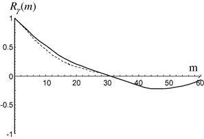
Figure 11.45 Normalized ACF of correlated Gamma variates. Dashed line: original data; solid line: simulated data.
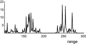
Figure 11.46 Correlated Gamma variates, with normalized ACF of Figure 11.45.
This method can readily be extended to two dimensions, as described in [25,75].
In some situations, particularly for detection purposes, we may be interested in generating many independent vectors of correlated compound-Gaussian clutter. If the Time-on-Target (ToT) is short (tens of ms) the texture can be considered a constant in each vector but randomly changing from one vector to the other. In this case, the compound-Gaussian model degenerates into the Spherically Invariant Random Process (SIRP), proposed by Conte and Longo [12] for modeling the radar sea clutter. The samples of the SIRV constitutes a spherically invariant random vector (SIRV) whose PDF is given by
 (11.88)
where the vector ![]() is the vector we want to generate. Then the vector
is the vector we want to generate. Then the vector ![]() we need is the product between the texture real random variable
we need is the product between the texture real random variable ![]() and a speckle complex Gaussian vector
and a speckle complex Gaussian vector ![]() . Conditionally to the texture, the covariance matrix of the vector
. Conditionally to the texture, the covariance matrix of the vector ![]() is the covariance matrix M of the speckle. The problem is then reduced to the generation of a Gaussian vector with a certain covariance matrix M. To this purpose, we can use a linear filter as described at the beginning of this section (sequential method), or a batch method based on the invariance property of the Gaussian processes with respect to linear operations. Consider the vector
is the covariance matrix M of the speckle. The problem is then reduced to the generation of a Gaussian vector with a certain covariance matrix M. To this purpose, we can use a linear filter as described at the beginning of this section (sequential method), or a batch method based on the invariance property of the Gaussian processes with respect to linear operations. Consider the vector ![]() where w is a vector of independent identically distributed complex Gaussian random variables with zero-mean and unit variance. The covariance matrix of x is
where w is a vector of independent identically distributed complex Gaussian random variables with zero-mean and unit variance. The covariance matrix of x is ![]() . There are many ways to find a matrix A satisfying this relation. One of them is the Cholesky decomposition that results in a lower triangular matrix A=L [78]. Summarizing, to generate the vector
. There are many ways to find a matrix A satisfying this relation. One of them is the Cholesky decomposition that results in a lower triangular matrix A=L [78]. Summarizing, to generate the vector ![]() with must generate first w, multiply it by the matrix A and then by the random variable
with must generate first w, multiply it by the matrix A and then by the random variable ![]() . The advantage of this method with respect to the sequential one is that it does not suffer the problem of the transient term.
. The advantage of this method with respect to the sequential one is that it does not suffer the problem of the transient term.
2.11.5 Use of clutter models in radar design and analysis
2.11.5.1 Performance prediction
One of the purposes of clutter models is to predict the performance of radar systems. This is typically achieved by initial application of the radar equation to establish the relative power levels for a given situation of returns from targets and clutter and thermal noise.
The basic radar equation for noise-limited target detection performance can be written as
![]() (11.89)
(11.89)
where
![]() Standard noise temperature, 290K.
Standard noise temperature, 290K.
The basic radar hardware and waveform parameters can be measured accurately in the factory. The system losses will usually include the microwave losses in the radar hardware, which can be measured, and the propagation losses, which usually cannot be measured but must be estimated from the prevailing conditions and models. It is sometimes convenient to include signal processing “losses” in this term to account for the non-ideal nature of subsequent signal processing compared with some idealized form used to calculate performance analytically.
For a single pulse return, detection performance can be described in terms of the probability of false alarm, ![]() , and probability of detection,
, and probability of detection, ![]() , following a detection threshold. For a square law detector, Gaussian clutter and an idealized fixed threshold detection threshold, t:
, following a detection threshold. For a square law detector, Gaussian clutter and an idealized fixed threshold detection threshold, t:
![]() (11.90)
(11.90)
For a Swerling Case 1 or Case 2 target ([79], exponential PDF), with mean power s
 (11.91)
where ![]() , the signal-to-noise ratio.
, the signal-to-noise ratio.
For other target models, equivalent PDFs of target-plus-noise must be derived. For example, a non-fading target in noise results in a Rice PDF [33].
If the returns include clutter, then the clutter to noise ratio can be determined by replacing the target RCS by that of the clutter return, ![]() . As described in Section 2.11.2.1.1, for surface distributed clutter,
. As described in Section 2.11.2.1.1, for surface distributed clutter, ![]() . Appropriate values of
. Appropriate values of ![]() are usually derived from empirical models, as described in Section 2.11.2.2.1 and 2.11.2.3.1. The values of
are usually derived from empirical models, as described in Section 2.11.2.2.1 and 2.11.2.3.1. The values of ![]() and
and ![]() must now be calculated for a return that includes clutter-plus-noise. This requires a knowledge of the PDFs of the envelope of clutter-plus-noise and target-plus-clutter-plus-noise, which can sometimes be difficult to derive. For a known clutter PDF, the PDF of clutter-plus-noise will generally have to be calculated numerically. In the particular case of the compound K distribution model, the PDF of clutter-plus-noise can be defined exactly [80]. Similarly, the PDF of the envelope of target-plus-clutter-plus-noise is required to calculate
must now be calculated for a return that includes clutter-plus-noise. This requires a knowledge of the PDFs of the envelope of clutter-plus-noise and target-plus-clutter-plus-noise, which can sometimes be difficult to derive. For a known clutter PDF, the PDF of clutter-plus-noise will generally have to be calculated numerically. In the particular case of the compound K distribution model, the PDF of clutter-plus-noise can be defined exactly [80]. Similarly, the PDF of the envelope of target-plus-clutter-plus-noise is required to calculate ![]() . Again, this can be calculated for the compound K distribution model for a wide range of target fading models [25].
. Again, this can be calculated for the compound K distribution model for a wide range of target fading models [25].
2.11.5.1.1 Signal processing and design of detectors
The radar equation provides a means of calculating the signal-to-clutter-plus-noise ratio, SCNR, and the clutter-to-noise ratio, CNR, for a single pulse return. For many radar systems, the returns from several successive pulses are integrated, to benefit from more radar power on the target. These pulses may sometimes be at different frequencies (frequency agility). In a typical example, during a dwell on a target, a pulse Doppler radar may transmit a burst of pulses with a fixed PRF and frequency, followed by successive bursts at different PRFs and frequencies. Returns from trains of pulses are used in subsequent signal processing to improve target detection and discrimination against clutter and noise.
To calculate ![]() and
and ![]() following detection processing in the radar requires knowledge of the effect of the processing on the amplitude statistics immediately prior to the final detection threshold or decision. For coherent processing with Doppler filter banks (typically achieved with an FFT over a fixed frequency burst of pulses), the Doppler spectra of target and clutter must be known to calculate the subsequent SCNR and CNR in each Doppler filter. The outputs from each Doppler filter may then be detected and then subsequent detections from successive bursts may be non-coherently integrated. Again the PDF of the integrated signals must be calculated. In the case of clutter, it is very important to understand any correlation between the samples that are being integrated. Thermal noise will always be independent from pulse to pulse. For clutter, the situation is more complex, with different components fluctuating at different rates. For example, pulse-to-pulse frequency agility can decorrelate the speckle component of sea clutter [10], but the underlying mean level component is not affected and may effectively be constant over a dwell. The target returns may also fluctuate at different rates over a dwell. This type of behavior is usually approximated by estimating the effective number of independent samples observed over a dwell period. Again, for the compound K distribution model it is possible to model the effects of pulse-to-pulse integration taking into account the effective number of independent samples of target, thermal noise and the two clutter components, each of which may be different [25].
following detection processing in the radar requires knowledge of the effect of the processing on the amplitude statistics immediately prior to the final detection threshold or decision. For coherent processing with Doppler filter banks (typically achieved with an FFT over a fixed frequency burst of pulses), the Doppler spectra of target and clutter must be known to calculate the subsequent SCNR and CNR in each Doppler filter. The outputs from each Doppler filter may then be detected and then subsequent detections from successive bursts may be non-coherently integrated. Again the PDF of the integrated signals must be calculated. In the case of clutter, it is very important to understand any correlation between the samples that are being integrated. Thermal noise will always be independent from pulse to pulse. For clutter, the situation is more complex, with different components fluctuating at different rates. For example, pulse-to-pulse frequency agility can decorrelate the speckle component of sea clutter [10], but the underlying mean level component is not affected and may effectively be constant over a dwell. The target returns may also fluctuate at different rates over a dwell. This type of behavior is usually approximated by estimating the effective number of independent samples observed over a dwell period. Again, for the compound K distribution model it is possible to model the effects of pulse-to-pulse integration taking into account the effective number of independent samples of target, thermal noise and the two clutter components, each of which may be different [25].
The design of optimum and suboptimum, adaptive and non-adaptive, coherent and non-coherent detectors for detecting point-targets embedded in Gaussian disturbance is a mature and well understood topic. There are many excellent books and papers addressing different aspect of the problem. Some references are listed in [81]. Conversely, the detection of targets embedded in non-Gaussian clutter is a less mature topic, even though there are many references published in the last 20 years (see for instance [19,22,25,82–92] and references therein). The main problems that must be taken into account are the estimation of the disturbance covariance matrix, the estimation of the parameters of the clutter distribution [17,25,93–95], the non-stationarity of the clutter in the case of sea scattering [96] and the site-dependence of the clutter in the case of ground scattering [97,98]. New radar systems must be able to rapidly adapt to changing conditions. Knowledge or estimation of clutter conditions can assist with the selection of both transmitted waveforms and detection algorithms.
2.11.5.2 The specification and measurement of radar performance
Another important role for clutter models relates to the specification and measurement of real radar performance. This is discussed in detail in [4,25,99–101].
Modern radars, especially those that use adaptive processing, are extremely complex and their performance is difficult to specify. A customer needs to ensure that those features of the radar that will define its ability to achieve the required operational capability are adequately specified. The ability to do this is in turn dependent upon a detailed understanding of the likely radar performance in different environmental and operational conditions. The supplier, however, needs to have a simple set of performance criteria upon which to base the radar design. One way to bridge this gap is to use a model that relates the basic performance of the radar to its behavior in complex operational environments. An important component of such models is likely to be the behavior of radar clutter.
A typical radar life cycle involves the use of models by the customer, the supplier and the user at various times. Table 11.20 shows a typical range of applications for models [4] during a radar’s life.
Table 11.20
Applications of Clutter Models during the Life-Cycle of a Radar
| Modelers | Life-Cycle Stages | Requirements for Clutter Models |
| Customer | Requirements definition | Generic performance modeling; High level synthetic environment simulations |
| Customer and potential suppliers | Modeling of potential performance | Performance predictions of different designs Comparison of competing designs; |
| Supplier | System and algorithm design | Performance prediction; Algorithm design (insight from models); Algorithm simulation Hardware and software stimulation. |
| Customer and supplier | Performance assessment and acceptance trials | Analysis of trials data; comparison of trials results with performance predictions |
| Radar user | In-service tactics and training | Simulation and hardware stimulation |
| Customer, suppler and user | In-service upgrades | Performance predictions; Algorithm simulation; synthetic environment simulation |
2.11.5.2.1 Clutter models for performance acceptance and trials analysis
An increasingly important role for models is for the analysis of radar trials and the acceptance by a customer of a new radar into service.
Acceptance trials are an integral part of any radar development program. These are intended to demonstrate to the customer that the radar provides the required functionality and is “fit for purpose.” It is also usually desired that trials be used to quantify the key performance parameters of the radar (e.g., detection range against a given target type). However, in many cases the reliable measurement of performance on trials is very difficult and may at the very least require many hours of trials. This is particularly true for radars required to detect very small targets in difficult clutter conditions or for radars that are continuously adapting their parameters (such as signal processing, waveforms, antenna beamshape, etc.) in response to changing environmental conditions. The customer may specify that a target of given RCS must be detected at a certain range, in particular environmental conditions (rainfall rate, sea state, etc.). Given an agreed set of models, such a situation could be modeled and provide reasonably accurate estimates of performance, within the limitations of the models used. However, measurement of these parameters in a trial can be very difficult. Even the apparently simple task of measuring the noise-limited detection range of a moving target is not straightforward [102]. If the original requirement was, say, to detect a target in sea state 3, in 1mm/h of rain, the radar designer would have to put a very large margin on expected trials results to allow for uncertainty in assessing whether sea state three is present, what the rainfall rate was (at the target and over the intervening path), combined with the large range of clutter characteristics, such as ![]() associated with a given sea state. Although the radar designer would be able to model performance for given clutter model parameters, it would not usually be possible to relate these to the conditions actually prevailing on a trial.
associated with a given sea state. Although the radar designer would be able to model performance for given clutter model parameters, it would not usually be possible to relate these to the conditions actually prevailing on a trial.
One solution is to combine trials measurements with modeling and factory measurements. Factory measurements can determine the basic radar parameters that determine noise-limited performance in, say, clear air. Modeling can predict the expected mean performance for a wide range of target sizes and clutter characteristics, which could never be tested in practical trials of reasonable duration. The empirical models that are used in radar design have themselves been developed from many hours of trials data, representing an average expected conditions that do not then have to be reproduced in acceptance trials. Then on a trial, detection performance can be measured (detection range, for example) for the target and environmental conditions applying on the trial. At the same time, the raw radar returns can be recorded for subsequent analysis. This analysis can yield the actual target and clutter characteristics that were present, provided that the radar noise-limited performance is suitably calibrated. These observed characteristics can then be input to the performance prediction model with the results compared with those actually achieved in the trial.
If raw radar data is recorded on a trial, it should also be possible to replay it through the radar signal processing, to assess the effects of different detection algorithms. In addition, it may be possible to inject synthetic targets, to further investigate detection performance.
This type of approach, combining trials with performance prediction modeling, can allow quantitative assessment of performance that would be effectively impossible from trials alone (due to uncertainty over the prevailing conditions and the time and cost of extensive trials). Of course, it is far from straightforward to achieve. It implies the measurement of detection ranges and false alarms rates from trials observations, and the estimation of clutter and target characteristics from recorded data. Each of these measurements is subject to its own measurement errors and the combined results would have to be analyzed in detail to assess the buyer and seller risks [25] associated with eventual equipment acceptance or rejection. The analysis methods and also the underlying performance prediction model must be agreed in detail between customer and supplier (preferably well in advance of any acceptance trials actually take place).
2.11.6 Conclusions
Modeling and analysis of clutter, as described in this tutorial, is a very important and complex matter. The characteristics of clutter depend on the environmental conditions, the viewing geometry and the radar characteristics. In general, there are not unique empirical or theoretical models that exhibit a satisfactory fit to real data under all possible conditions. Nevertheless, we have shown some general trends focusing particularly on sea and ground clutter recorded by high resolution pulsed radars. For low grazing angles and high spatial resolution, sea clutter amplitude statistics are not Gaussian and the returns exhibit some distinct amplitude peaks, called spikes, that can be confused by a radar system for targets. The spikyness of sea clutter increases with resolution and is more evident in HH polarized data. A good and flexible statistical model for sea clutter is the compound-Gaussian model, which comprises among its particular cases the popular Rayleigh, Weibull and K models. One of the advantages of the compound-Gaussian model is its mathematical tractability that helps in designing optimum and suboptimum detectors and the possibility of describing separately the amplitude PDF and the correlation characteristics. For sea clutter, this family of distributions has been found to give a good fit over a wide range of conditions, although this model may sometimes fail at very high spatial resolutions. These models can also be used successfully for ground clutter, especially when the ground clutter is scattered by discrete objects as pylons, fences, tree trunks. In some scenarios, when the ground surface is covered by wind-blown trees and vegetation, the clutter still exhibits Gaussian statistics, even at high resolutions.
Concerning the clutter spectrum, many models have been proposed in the literature in the last 50years. We have presented some results with AR models, Gaussian, power law and exponential PSDs. Again, there is not a unique optimum model for all the conditions. The AR model is very flexible and shows a good fitting with sea clutter and ground clutter in some cases, but the exponential one seems to be the best for windblown tree clutter recorded by high dynamic-range radars.
Finally, we cannot make a “final point” or a definite conclusion on this complex matter because the study of clutter models is a continuing research topic. As radar systems improve, new features of clutter and target scattering may be observed and new analyses are then necessary to develop more accurate models of these characteristics and to improve the design of target detectors.
Relevant Theory: Signal Processing Theory
See Vol. 1, Chapter 4 Random Signals and Stochastic Processes
References
1. Nathanson FE. Radar Design Principles. McGraw Hill 1969.
2. Skolnik MI. Introduction to Radar Systems. third ed. McGraw Hill 2001.
3. Tait P. Introduction to Radar Target Recognition. IET 2006.
4. Ward KD, Watts S. Use of sea clutter models in radar design and development. IET Radar Sonar Navig. 2010;4(2):146–157 (Special Issue on Radar Clutter).
5. Watts S. Radar sea clutter modelling—recent progress and future challenges. In: International Radar Conference 2008, Adelaide. September 2008; (Invited Paper).
6. Blythe JM, Rice DE, Attwood WL. The CFE clutter model, with application to automatic detection. Marconi Rev. 1969;32:185–206.
7. G.R. Valenzuela, M.B. Lang, On the statistics of sea clutter, NRL, Report 7349, 1971.
8. Trunk GV. Radar properties of non-Rayleigh sea clutter. IEEE Trans AES. 1972;8:196–204.
9. Ward KD. Compound representation of high resolution sea clutter. Electron Lett. 1981;17:561–563.
10. Ward KD, Baker CJ, Watts S. Maritime surveillance radar Part 1: radar scattering from the ocean surface. Proc IEE. 1990;137(2):51–62 (part F).
11. Barnard TJ, Weiner DD. Non-Gaussian clutter modeling with generalized spherically invariant random vectors. IEEE Trans Signal Process. 1996;44.
12. Conte E, Longo M. Characterisation of radar clutter as a spherically invariant random process. IEE Proc.-F. 1987;134(2):191–197.
13. Conte E, De Maio A, Galdi C. Statistical analysis of real clutter at different range resolutions. IEEE Trans Aerosp Electron Syst. 2004;40(3):903–918.
14. Fay FA, Clarke J, Peters RS. Weibull distribution applied to sea-clutter. In: Proceedings of the IEE Conference Radar ’77, London, UK. 1977.
15. Farina A, Gini F, Greco M, Verrazzani L. High resolution sea clutter data: a statistical analysis of recorded live data. IEE Proc.-F. 1997;144(3):121–130.
16. Jakeman E, Pusey PN. A model for non-Rayleigh sea echo. IEEE Trans Antenna Propag. 1976;AP-24:806–814.
17. Rangaswamy M, Weiner DD, Ozturk A. Non-Gaussian vector identification using spherically invariant random processes. IEEE Trans Aerosp Electron Syst. 1993;29(1):111–124.
18. Rangaswamy M, Weiner DD, Ozturk A. Computer generation of correlated non-Gaussian radar clutter. IEEE Trans Aerosp Electron Sys. 1995;31(1):106–115.
19. Rangaswamy M, Michels JH, Weiner DD. Multichannel detection algorithm for correlated non-Gaussian random processes based on innovations. IEEE Trans Signal Process. 1995;43(8):1915–1922.
20. Rangaswamy M, Michels JH. A parametric multichannel detection for correlated non-Gaussian random processes. In: Proceedings of the National Radar Conference, Syracuse, NY, USA. May 1997;349–354.
21. Rangaswamy M, Michels JH. Adaptive signal processing in non-Gaussian noise backgrounds. In: Proceedings of the Nineth IEEE-SSAP Workshop, Portland, OR. September 1998.
22. Sangston KJ, Gerlach KR. Coherent detection of radar targets in a non-Gaussian background. IEEE Trans Aerosp Electron Syst. 1994;30(2):330–340.
23. Sekine M, Mao Y. Weibull Radar Clutter. London: Peter Peregrinus Ltd.; 1990.
24. Middleton D. New physical-statistical methods and models for clutter and reverberation: the KA distribution and related probability structures. IEEE J Oceanic Eng. 1999;24(3):261–284.
25. Ward KD, Tough RJA, Watts S. Sea Clutter: Scattering, the K Distribution and Radar Performance. Institution of, Engineering and Technology 2006.
26. Pidgeon VW. Doppler dependence of radar sea return. J Geophys Res. 1968;73:1333–1341.
27. Lee PHY, Barter JD, Beach KL, et al. X-band microwave backscattering from ocean waves. J Geophys Res. 1995;100(C2):2591–2611.
28. Lee PHY, Barter JD, Beach KL, et al. Power spectral lineshapes of microwave radiation backscattered from sea surfaces at small grazing angles. lEE Proc F. 1995;142(5):252–258.
29. Billingsley JB, Farina A, Gini F, Greco M, Verrazzani L. Statistical analyses of measured radar ground clutter data. IEEE Trans Aerosp Electron Syst. 1999;35(2):579–593.
30. Haykin S, Steinhardt A. Adaptive Radar Detection and Estimation. New York: Wiley; 1992.
31. CSIR, small boat detection research, <http://www.csir.co.za/smallboatdetection/>.
32. Billingsley JB. Low-Angle Radar Land Clutter—Measurements and Empirical Models. Norwich, NY: William Andrew Publishing; 2002.
33. Barton DK. Radar System Analysis and Modeling. Artech House 2005.
34. Long WHD, Mooney D, Skillman WA. Pulse Doppler radar. In: Skolnik M, ed. Radar Handbook. second ed. New York: McGraw Hill; 1990;17.11–17.16. (Chapter 17).
35. Rosenberg L, Crisp DJ, Stacy NJ. Analysis of the kk-distribution with medium grazing angle sea-clutter. IET Proc Radar Sonar Navig. 2010;4:209–222.
36. Wright JW. A new model for sea clutter. IEEE Trans AP. 1968;16:217–223.
37. Bass FG, Fuks IM, Kalmykov AE, Ostrovsky IE, Rosenberg AD. Very high frequency radiowave scattering by a disturbed sea surface. IEEE Trans Antenna Propag. 1968;AP-16:554–568.
38. Gerstoft P, Rogers LT, Wagner LJ, Hodgkiss WS. Estimation of radio refractivity structure using radar clutter. In: 30th International Conference on Radar Meteorology, München Germany. July 2001;19–24.
39. Horst MM, Dyer FB, Tuley MT. Radar sea clutter model. In: IEEE International Conference Antennas and Propagation. November 1978;6–10.
40. Wetzel LB. Sea Clutter. In: Skolnik M, ed. Radar Handbook. second ed. New York: McGraw Hill; 1990; (Chapter 13).
41. Greco M, Bordoni F, Gini F. X-band sea clutter non-stationarity: the influence of long waves. IEEE J Ocean Eng. 2004;29(2):269–283 (Special Issue on Non-Rayleigh Reverberation and Clutter).
42. Watts S. A new method for the simulation of coherent sea clutter. In: IEEE International Conference, RadarCon 2011. May 2011.
43. Ritchie MA, Woodbridge K, Stove AG. Analysis of sea clutter distribution variation with Doppler using the compound K-distribution. In: International Conference on IEEE Radar 2010. May 2010;495–499.
44. R.R. Boothe, The Weibull distribution applied to the ground clutter backscattering coefficient, US Army Missile Command, RE-TR-69-15, ADA691109, 1969.
45. Long MW. Radar reflectivity of Land and Sea. third ed. Artech House 2001.
46. Moore RK. Ground echo. In: Skolnik M, ed. Radar Handbook. third ed. New York: McGraw Hill; 2008; (Chapter 16).
47. Ulaby FT, Dobson MC. Handbook of Radar Scattering Statistics for Terrain. Norwood MA: Artech House; 1989.
48. Currie NC. Clutter characteristics and effects. In: Eaves JL, Ready EK, eds. Principles of Modern Radar. New York: Van Nostrand Reinhold; 1987;281–340.
49. Morchin WC. Airborne Early Warning Radar. Artech House 1990.
50. Blake LV. Prediction of radar range. In: Skolnik M, ed. Radar Handbook. first ed. McGraw Hill 1970.
51. Greco M, Gini F, Rangaswamy M. Statistical analysis of real polarimetric clutter data at different range resolutions. IEE Proc Radar Sonar Navig. 2006.
52. B. Currie, Private, Communications, October 2003.
53. Kay SM. Fundamentals of Statistical Signal Processing. Estimation Theory. vol. I Prentice Hall 1993.
54. Lehmann EL. Testing Statistical Hypotheses. second ed. New York: Springer texts in statistics; 2010.
55. Nohara T, Haykin S. Canadian East coast radar trials and the K-distribution. IEE Proc.-F. 1991;F138(2):80–88.
56. Sadler B, Giannakis GB, Lii KS. Estimation and detection in the presence of non-Gaussian noise. IEEE Signal Process. 1994;42(10):2729–2741.
57. Gini F. A Cumulant-based adaptive technique for coherent radar detection in a mixture of K-distributed clutter and Gaussian disturbance. IEEE Trans Signal Process. 1997;45(6):1507–1519.
58. Gini F, Greco M. Texture modelling, estimation, and validation using measured sea clutter data. IEE Proc Radar Sonar Navig. 2002;149.
59. Haykin S, Bakker R, Currie BW. Uncovering nonlinear dynamics—the case study of sea clutter. Proceedings of the IEEE. 2002;90(5):860–881.
60. Valenzula GR. Theories for the interaction of electromagnetic waves and oceanic waves—a review, bound. Layer Meteorol. 1978;13(1–4):61–65.
61. Plant WJ, Keller WC. Evidence of Bragg scattering in microwave Doppler spectra of sea return. J Geophys Res. 1990;95(C9):16299–16310.
62. Plant WJ, Keller WC. The two-scale radar wave probe and SAR imagery of the ocean. J Geophys Res. 1983;88(C14):9776–9784.
63. Rino CL, Eckert E, Siegel A, et al. X-band low-grazing-angle ocean backscatter obtained during LOGAN 1993. IEEE J Oceanic Eng. 1997;22(1):18–26.
64. Rozenberg AD, Quigley DC, Melville WK. Laboratory study of polarized microwave scattering by surface waves at grazing incidence: the influence of long waves. IEEE Trans Geosci Remote Sens. 1996;34(6):1331–1342.
65. Walker D. Experimentally motivated model for low grazing angle radar Doppler spectra of the sea surface. IEE Proc Radar Sonar Navig. 2000;147(3):114–120.
66. Walker D. Doppler modelling of radar sea clutter. IEE Proc Radar Sonar Navig. 2001;148.
67. Trizna DB. A model for Doppler peak spectral shift for low grazing angle sea scatter. IEEE J Oceanic Eng. 1985;10(4):368–375.
68. Jessup AT, Melville WK, Keller WC. Breaking waves affecting microwave backscatter 1 Detection and verification. J Geophys Res. 1991;96(C11):20547–20559.
69. A. Drosopoulos, Description of the OHGR database, Technical Note No. 94–14, Defence Research Establishment Ottawa, December 1994.
70. Haykin S. In: Englewood Cliffs, NJ 07632: Prentice Hall; 1991;Haykin Simon, ed. Advances in Spectrum Analysis and Array Processing. vol. I.
71. Therrien CW. Discrete Random Signals and Statistical Signal Processing. Englewood Cliffs, NJ 07632: Prentice Hall; 1992.
72. Kim PJ, Jennrich RI. Tables of the exact sampling distribution of the two sample Kolmogorov-Smimoff criterion (Dmn < m <n). In: Providence, RI: American Mathematical Society; 1973;Harter HL, Owen DB, eds. Selected Tables in Mathematical Statistics. vol. I.
73. Greco M, Gini F, Farina A, Billingsley JB. Validation of windblown ground clutter spectral shape by analysis of clutter cancellation in the presence of measured clutter data. IEEE Trans Aerosp Electron Syst. 2001;37(2):538–548.
74. Chen KS, Fung AK. Frequency dependence of backscattered signals from forest components. IEE Proceedings, Pt F. 1995;142(6):310–315.
75. Tough RJA, Ward KD. The correlation properties of gamma and other non-Gaussain processes generated by memoryless nonlinear transformation. J Phys D. 1999;32:3075–3084.
76. Farina A, Russo A, Studer FR. Coherent radar detection in log-normal clutter. IEE Proc.-F. 1986;133(1):39–54.
77. Farina A, Russo A, Scannapieco F, Barbarossa S. Theory of radar detection in coherent Weibull clutter. IEE Proc.-F. 1987;134(2):174–190.
78. Golub Gene H, Van Loan Charles F. Matrix computations. third ed. Johns Hopkins University Press 1996; (Section 4.2, ISBN: 0-8018-5414-8).
79. Swerling P. Probability of detection for fluctuating targets. IRE Trans IT-6. 1960;269–308.
80. Watts S. Radar detection prediction for targets in both K-distributed sea clutter and thermal noise. IEEE Trans. 1987;AES-23(2):40–45.
81. Gini F, Farina A, Greco M. Selected list of references on non-Gaussian radar detection. IEEE Trans Aerosp Electron Syst. 2001;37(1):329–359.
82. Conte E, Ricci G. Performance prediction in compound-Gaussian clutter. IEEE Trans Aerosp Electron Syst. 1994;30(2):611–616.
83. Conte E, Lops M, Ricci G. Asymptotically optimum radar detection in compound-Gaussian clutter. IEEE Trans Aerosp Electron Syst. 1995;31(2):617–625.
84. Conte E, De Maio A, Galdi C. Signal detection in compound-Gaussian noise: Neyman-Pearson and CFAR detectors. IEEE Trans Signal Process. 2000;48(2):419–428.
85. Gini F, Greco MV, Farina A, Lombardo P. Optimum and mismatched detection against K-distributed plus Gaussian clutter. IEEE Trans Aerosp Electron Syst. 1998;34(3):860–876.
86. Gini F, Greco M. A suboptimum approach to adaptive coherent radar detection in compound-Gaussian clutter. IEEE Trans Aerosp Electron Syst. 1999;35(3):1095–1104.
87. Gini F, Greco M, Farina A. Clairvoyant and adaptive signal detection in non-Gaussian clutter: a data-dependent threshold interpretation. IEEE Trans Signal Process. 1999;47(6):1522–1531.
88. Haykin S, Thomson DJ. Signal detection in nonstationary environment reformulated as an adaptive pattern classification problem. Proceedings of the IEEE. 1998;86(11):2325–2344.
89. Richmond CD. Performance of a class of adaptive detection algorithms in non-homogeneous environment. IEEE Trans Signal Process. 2000;48(5):1248–1262.
90. Sangston KJ, Gini F, Greco M, Farina A. Structures for optimum and suboptimal coherent radar detection in compound-Gaussian clutter. IEEE Trans Aerosp Electron Syst. 1999;35(2):445–458.
91. Sangston KJ, Gini F, Greco M. Coherent radar detection in heavy-tailed compound-Gaussian clutter. IEEE Trans Aerosp Electron Syst. 2012;42(1):64–77.
92. Watts S, Baker CJ, Ward KD. Maritime surveillance radar Part 2: Detection performance prediction in sea clutter. IEE Proceedings-F. 1990;137:63–72.
93. Iskander DR, Zoubir AM. Estimation of the parameters of the K-distribution using higher order and fractional moments. IEEE Trans Aerosp Electron Syst. 1999;35(4):1453–1457.
94. Lombardo P, Oliver CJ. Estimation of texture parameters in K-distributed clutter. IEE Proc F. 1994;141(4):196–204.
95. Raghavan RS. A method for estimating parameters of K-distributed clutter. IEEE Trans Aerosp Electron Syst. 1991;27(2):238–246.
96. Greco M, Stinco P, Gini F, Rangaswamy M. Impact of sea clutter non-stationarity on disturbance covariance matrix estimation and CFAR detector performance. IEEE Trans Aerosp Electron Syst. 2010;46(3):1502–1513.
97. Griffiths HD. Knowledge-based solutions as they apply to the general radar problem. In: Proceedings of the RTO NATO Lecture Series 233 on Knowledge-Based Radar Signal and Data Processing, Rome, Italy. November, 2003;6–7.
98. Lops M. Hybrid clutter-map/L-CFAR procedure for clutter rejection in nonhomogeneous environment. IEE Proc.-F. 1996;143:239–245.
99. Watts S. Specification and measurement of performance for airborne maritime surveillance radars. In: International Radar Conference 1999, Brest. May, 1999;17–21. (Session 2.6).
100. S. Watts, H.D. Griffiths, J.R. Holloway, A.M. Kinghorn, D.G. Money, D.J. Price, A.M. Whitehead, A.R. Moore, M.A. Wood, D.J. Bannister, The specification and measurement of radar performance, in: International Radar, 14–17 October 2002, IEE, Publication No.490, pp. 542–546.
101. Watts S, Griffiths HD, Holloway JR, et al. The specification and measurement of radar performance—future research challenges. J Defence Sci. 2003;8(2):83–91.
102. Stove AG, Hurd DL. Performance evaluation for modern radars. In: Proceedings of IEEE International Radar Conference, Adelaide. September 2003;547–553. (paper 44).
1Results for different polarizations can be compared with respect to the mean value ![]() of the estimates
of the estimates ![]() of parameter
of parameter ![]() of the Weibull distribution, because the meaning of this parameter is quite easy to understand.
of the Weibull distribution, because the meaning of this parameter is quite easy to understand.
2For the definition of cumulants and their relation with the moments see [56]. Particularly, for real processes ![]() .
.