
Multitarget Multisensor Tracking
X. Chen, R. Tharmarasa and T. Kirubarajan, ECE Department, McMaster University, Hamilton, Ontario, Canada
Abstract
Multitarget-Multisensor tracking is a category of widely used techniques that are applicable to fields like air traffic control, air/ground/maritime surveillance, transportation, video monitoring and biomedical imaging/signal processing. In this chapter, various multitarget-multisensor tracking algorithms to handle state estimation, data association, track initialization, spatial clutter intensity estimation, debaising, and multisensor fusion in centralized/distributed/decentralized architecture are discussed in detail, including their quantitative and qualitative merits. In addition, several evaluation metrics are presented to measure the performance of different multitarget-multisensor tracking systems. Various combinations of these algorithms and performance evaluation metrics will provide a complete tracking and fusion framework for multisensor networks with application to civilian as well as military problems. The application of some of these algorithms and performance evaluation metrics is demonstrated on a representative real scenario, where several closely spaced targets are tracked using a radar system.
Keywords
Multitarget tracking; Multisensor fusion; Bayesian filtering; Clutter estimation; Tracklet; Data association
3.15.1 Introduction
Multisensor-multitarget tracking is an emerging technology in which measurements from several sensors are combined such that resulting tracks are significantly better than that obtained when these devices operate individually. Recent advances in sensor technologies, signal processing techniques and improved processor capabilities make it possible for large amounts of data to be fused in real-time. These technical advancements allow the use of many sophisticated algorithms and robust mathematical techniques in multisensor-multitarget tracking. Furthermore, multisensor-multitarget tracking has received significant attention for military applications. Such applications involve a wide range of expertise including filtering, tracking initialization and maintenance, data association, and performance evaluation.
Three major types of architecture, namely, centralized, distributed and decentralized, are commonly used in multisensor-multitarget tracking applications [9,62,92,126]. In the centralized architecture, there are several sensors monitoring the region of interest with only one fusion center. All sensors report their measurements to the fusion center. It is the fusion center’s responsibility to process all acquired measurements and update the tracks. The single sensor-multitarget tracking problem can be considered as a special case of the centralized architecture, where only one sensor is deployed to observe the region of interest. In the distributed multisensor-multitarget tracking architecture, there are several fusion centers. One of them is the Central Fusion Center (CFC) and the remaining ones are Local Fusion Centers (LFCs). Measurements generated by the sensors are first processed by the LFCs and local tracks are updated inside each LFC. Then, local tracks from each LFC are reported to the CFC and the track-to-track fusion is accomplished by the CFC to form the global track set. In decentralized tracking architecture, each fusion center (FC) can be considered as a combination of LFC and CFC. Each FC is connected with several sensors and measurements reported by those sensors are used to update the track state inside the FC. Furthermore, each FC will also do track-to-track fusion whenever it receives additional information from its neighboring FCs. Usually, without a major modification, the algorithms developed for the distributed tracking architecture can be used to handle the decentralized tracking architecture. Regardless whether the sensor measurements are processed in the centralized or the distributed architecture, the data of each sensor has to be converted to a common coordinate system before multisensor-multitarget tracking, i.e., sensor registration and data alignment [39,54,74].
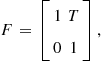
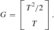
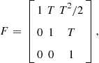
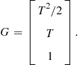
Filtering plays a vital role in multitarget tracking by obtaining the state estimate from the measurements received from one or more sensors. Tracking filters [10,31] can be broadly categorized as either linear or nonlinear. The Kalman filter [10,53] is a widely known recursive filter that is most suited for linear Gaussian systems. However, most systems are inherently nonlinear. The extensions of Kalman filter, such as extended Kalman filter (EKF) [10] and unscented Kalman filter (UKF) [52,105,128] are applicable to nonlinear systems. Both EKF and UKF are restricted in that the resulting probability densities are approximated as Gaussian. When the system is nonlinear and non-Gaussian, particle filters (or sequential Monte Carlo methods) [3,33,38,100] provide better estimates than many other filtering algorithms. In general, a tracking filter requires a model for target dynamics, and a model mismatch would diminish the performance of the filter. Thus, different models may be required to describe the target dynamics accurately at different times, especially in the case of maneuvering targets, whose kinematic models may evolve in a time-varying manner. Multiple model tracking algorithms such as the Interacting Multiple Model (IMM) [1,10,14–16,18] estimator, which contains a bank of models matched to different modes of possible target dynamics, would perform better in such situations.
Data association [9,13,113] is an essential component in multisensor-multitarget tracking due to the uncertainty in the data origin. Data association refers to the methodology of correctly associating the measurements to tracks, measurements to measurements [58,106] or tracks to tracks [2,6,8,9,19,22,127], depending on the fusion architecture. To address data association, a number of techniques have been developed and two widely used are single-frame assignment algorithm [11,95] and the multi-frame assignment algorithm [11,17,27,32,59,63,95].
Many algorithms have been proposed for the single sensor-multitarget tracking problem, such as the Probability Data Association (PDA) algorithm and the Joint Probability Data Association (JPDA) algorithm [9], the Multiple Hypotheses Tracking (MHT) algorithm [12], and the Probability Hypothesis Density (PHD) filter [78]. In PDA and JPDA algorithms, for each scan the track-to-measurement association events are enumerated and combined probabilistically, while in the MHT algorithm the track-to-measurement association history over several scans are enumerated and updated. In PHD filter, the track-to-measurement association events are not explicitly constructed. Although these algorithms are originally proposed to handle the single sensor-multitarget tracking problem, they are also widely used as the backbone for the multisensor-multitarget tracking.
In many scenarios, after the signal detection process, clutter points provided by the sensor (e.g., sonar, infrared sensor, radar) are not distributed uniformly in the surveillance region as assumed by most tracking algorithms. On the other hand, in order to obtain accurate results, the target tracking filter requires information about clutter’s spatial intensity. Thus, nonhomogeneous clutter spatial intensity has to be estimated from the measurement set and the tracking filter’s output. Also, in order to take advantage of existing tracking algorithms, it is desirable for the clutter estimation method to be integrated into the tracker itself.
Performance evaluation is very important for multisensor-multitarget tracking problem, especially when the performance of different tracking algorithms needs to be compared. Many measures of performance have been proposed in multisensor-multitarget tracking literatures. These measures can be divided into two different classes: sensor-related measures and tracker-related measures [40]. Sensor-related measures are independent of the tracking algorithm, therefore, most of them are not useful for the performance evaluation of multiple trackers. One exception is the Posterior Cramér-Rao Lower Bound (PCRLB) of tracking [10,44,46], which provides a minimum bound of any tracking estimation. On the other hand, tracker-related measures have been widely used in the tracker performance evaluation. For general multitarget tracking problem, tracker-related measures have been defined in terms of cardinality, time and accuracy measures [66,103]. To evaluate a general multitarget tracking problem, a combination of tracker-related measures should be used, because as shown in [29], it has been observed that the tracker may have provided inaccurate results while some measures show correct and satisfactory performances.
In this chapter, various multisensor-multitarget tracking architectures, estimators for spatial clutter intensity, filters for linear and nonlinear systems, algorithms for data associations and multitarget tracking, techniques used in centralized and distributed track-to-track fusion are discussed in detail. In addition, their quantitative and qualitative merits are discussed. Various combinations of these algorithms will provide a complete tracking framework for multisensor networks with application to civilian as well as military problems. For example, the tracking and fusion techniques discussed here are applicable to fields like air traffic control, air/ground/maritime surveillance, mobile communication, transportation, video monitoring and biomedical imaging/signal processing. The tracker performance evaluation, including its guiding principle and several measures of performance, is also discussed in this chapter. A challenging scenario with many closely-spaced targets is used to compare several multitarget tracking algorithms.
3.15.2 Formulation of multisensor-multitarget tracking problems
In a multisensor surveillance systems, several sensors such as radar, infrared (IR), and sonar, report their measurements to the tracker at regular intervals of time (scans or data frames). However, not all measurements are originated from the targets of interest; some measurements may come from physical background objects such as clutter, and others may be generated by thermal noise. In other words, there is a measurement origin ambiguity. Furthermore, in some scans, the target of interest does not produce any measurements at all (i.e., the probability of detection is less than unity). The objective of a typical multisensor-multitarget tracking system is to first partition all sensors’ measurements into sets, such that all observations in one set are produced by the same object (i.e., data-association process); then the measurements corresponding to the same object are processed in order to estimate the state of the object (i.e., filtering process) [9,12].
To handle the multisensor-multitarget tracking problem, usually the Bayesian approach is applied. In the Bayesian approach, the final goal is to construct the posterior probability density function (pdf) of the multitarget state given all the received measurements so far. Since this pdf contains all available statistical information, it is the complete solution to the multisensor-multitarget tracking problem. In principle, given a cost function, it is always possible to obtain the optimal estimate under the given cost function from the posterior probability. Note that, the state of the multitarget system should be a combination of the number of the targets and the state of each target, because in a real scenario both of them are random and unknown [78,120].
To distinguish the target-originated measurements from the clutter and estimate the state of the multitarget system, the following three models, namely, the target dynamic model, the sensor model, and the clutter model are crucial for all multisensor-multitarget tracking systems.
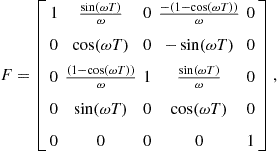
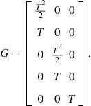
3.15.2.1 Target dynamic models
Target dynamic model, which is also known as system model, describes the evolution of the state with time, and is given by
![]() (15.1)
(15.1)
where ![]() is, in general, a nonlinear function,
is, in general, a nonlinear function, ![]() is the state of the target, and
is the state of the target, and ![]() is the process noise, which is usually assumed to be Gaussian. The covariance of the process noise multiplied by the gain
is the process noise, which is usually assumed to be Gaussian. The covariance of the process noise multiplied by the gain ![]() is
is
![]() (15.2)
(15.2)
The following models are widely used by the multitarget tracker as the target dynamic model: [10]
• Constant velocity:
The state vector in one generic coordinate is
![]() (15.3)
(15.3)
The ![]() and
and ![]() in one generic coordinate are
in one generic coordinate are
 (15.4)
 (15.5)
The process noise standard deviation ![]() is
is
![]() (15.6)
(15.6)
where ![]() is the scaling factor and
is the scaling factor and ![]() is the maximum acceleration.
is the maximum acceleration.
• Constant acceleration:
The state vector in one generic coordinate is
![]() (15.7)
(15.7)
The ![]() and
and ![]() in one generic coordinate are
in one generic coordinate are
 (15.8)
 (15.9)
The process noise standard deviation ![]() is
is
![]() (15.10)
(15.10)
• Coordinated turn:
The state vector is
![]() (15.11)
(15.11)
The ![]() and
and ![]() are
are
 (15.12)
 (15.13)
The process noise standard deviations ![]() and
and ![]() are
are
![]() (15.14)
(15.14)
![]() (15.15)
(15.15)
where ![]() and
and ![]() are the scaling factors for velocity and turn rate, respectively,
are the scaling factors for velocity and turn rate, respectively, ![]() is the maximum turn rate change in unit time.
is the maximum turn rate change in unit time.
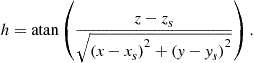
3.15.2.2 Sensor models
Sensor model, which is also known as measurement model, is a model relating the noisy measurements to the state and given by
![]() (15.16)
(15.16)
where ![]() is, in general, nonlinear functions,
is, in general, nonlinear functions, ![]() is the state of the target,
is the state of the target, ![]() is the measurement vector, and
is the measurement vector, and ![]() is the measurement noise at measurement time
is the measurement noise at measurement time ![]() , which is usually assumed to be Gaussian. The following measurement models are typical for the multisensor-multitarget tracking system:
, which is usually assumed to be Gaussian. The following measurement models are typical for the multisensor-multitarget tracking system:
![]() (15.17)
(15.17)
![]() (15.18)
(15.18)
![]() (15.19)
(15.19)
![]() (15.20)
(15.20)
For 2D tracking, the terms related to ![]() must be deleted.
must be deleted.
![]() (15.21)
(15.21)
For 2D tracking, the terms related to ![]() must be deleted.
must be deleted.
![]() (15.22)
(15.22)
![]() (15.23)
(15.23)
 (15.24)
 (15.25)
![]() (15.26)
(15.26)
![]() (15.27)
(15.27)
In (15.27),
![]()
3.15.2.3 A clutter model
For a sensor with ![]() resolution cells, sometimes detections will be declared in those cells that are pointed to a region without any targets of interest. The detection, which is not produced by any targets of interest, is know as a false alarm (i.e., clutter). Assume:
resolution cells, sometimes detections will be declared in those cells that are pointed to a region without any targets of interest. The detection, which is not produced by any targets of interest, is know as a false alarm (i.e., clutter). Assume:
• The events of detection in each cell is independent of each other.
• The probability of false alarm is equal to ![]() in each cell and
in each cell and ![]() .
.
Then the probability mass function (pmf) of the number of false alarm in these ![]() resolution cells,
resolution cells, ![]() , is approximately following the Poisson distribution [9]
, is approximately following the Poisson distribution [9]
![]() (15.28)
(15.28)
Furthermore, the spatial distribution of the false alarm is uniform based on the above three assumptions. Thus, if the granularity due to the size of the resolution cells can be neglected, the pdf of a false measurement, i.e., the clutter spatial intensity normalized by the expected number of clutter in the measurement space, is [9]
![]() (15.29)
(15.29)
where ![]() represents the volume of the sensor’s measurement space. The un-normalized clutter spatial intensity is
represents the volume of the sensor’s measurement space. The un-normalized clutter spatial intensity is
![]() (15.30)
(15.30)
3.15.2.4 Spatial clutter intensity estimation
Many target tracking algorithms assume that the clutter background is known or at least homogeneous. However, in real tracking problems, the distribution of clutter is often unknown and spatially non-homogeneous. Thus, there is usually a mismatch between the true spatial distribution of clutter points and the spatial distribution model used in the tracking filter. This mismatch may result in a high false track acceptance rate or a long delay of track initialization. Therefore, it is desirable for the tracking filter to estimate the spatial intensity of clutter from the measurement set. Also, due to the fact that target-originated measurement points and clutter points are indistinguishable before data association in the tracker, the output of tracking filter should also be used in order to get an unbiased estimate of clutter spatial intensity. Furthermore, estimation methods for clutter spatial distribution should be compatible with the existing target tracking algorithms, otherwise their application range would be limited.
One way to estimate clutter spatial intensity is to assume that clutter points are uniformly distributed in the validation gate and then use the sample spatial intensity as the estimate of clutter’s spatial intensity [9]. However, this method is based on the current measurement set alone and its performance relies on the volume of validation gate. For example, if the gate is so small that there are only a few measurements falling in it, the estimate of clutter’s spatial intensity may suffer from a large variance; on the other hand, if the gate is too large, then the uniform distribution assumption of clutter points may no longer hold. Also, this estimation method is biased, since it does not take into account target-originated measurements in the gate. In [67], in order to obtain an unbiased estimator of clutter’s spatial intensity, “track perceivability,” the probability that the target exists at the current time given all previous measurement [68], was used to handle target-originated measurements in the current measurement set.
In [43,87], the surveillance region was divided into sectors and clutter points in each sector were assumed to follow Poisson point processes. Based on the Poisson point processes assumption, three clutter spatial intensity estimators were discussed: the first one was based on the number of measurements falling in each sector, the second was based on each sector’s nearest neighbor measurement distance, which is equal to the distance from the center of the sector to its nearest measurement point, while the third was based on the inter-arrival time between two consecutive measurements falling in the same sector. In all three estimators, after obtaining the clutter intensity estimate based on the current measurement set, a time-averaging filter was used to smooth the clutter intensity estimate over time.
In [81,82], it was assumed that there are several unknown targets, called clutter generators, in a space which is disjoint from both the state space and the measurement space. All clutter points are generated by the clutter generator and an approximated Bayesian estimation method for the density of the clutter generator and the clutter is proposed. However, the proposed method is intractable and no practical implementation method was given in [81,82].
In [23], based on Poisson point processes, two methods for joint non-homogeneous clutter background estimation and multitarget tracking were presented. In that paper, non-homogeneous Poisson point processes, whose intensity function are assumed to be a mixture of Gaussian functions, were used to model clutter points. Based on this model, a recursive maximum likelihood method and an approximated Bayesian method using Normal-Wishart conjugate prior-posterior pair were proposed to estimate the non-homogeneous clutter spatial intensity. Both clutter estimation methods were integrated into the Probability Hypothesis Density (PHD) filter, which itself also uses the Poisson point process assumption. The mean and the covariance of each Gaussian function were estimated and used to calculate the clutter density in the update equation of the PHD filter. Simulation results showed that both methods were able to improve the performance of the PHD filter in the presence of slowly time varying non-homogeneous clutter background.
3.15.3 Filters
Filtering is the estimation of the state of a dynamic system from noisy data, based on the predefined target dynamic model and the sensor model. In recursive filtering, the received measurements are processed sequentially rather than as a batch so that it is neither necessary to store the complete measurement set nor to reprocess existing measurement if a new measurement becomes available. The Bayesian recursive filter is widely used in the multisensor-multitarget tracking area and such a filter consists of two stages: prediction and update.
The prediction stage uses the system model to predict the state pdf forward from one measurement time to the next. Suppose that the required pdf ![]() at measurement time
at measurement time ![]() is available, where
is available, where ![]() . The prediction stage involves using the system model (15.1) to obtain the prior pdf of the state at measurement time
. The prediction stage involves using the system model (15.1) to obtain the prior pdf of the state at measurement time ![]()
![]() (15.31)
(15.31)
The update stage uses the latest measurement ![]() to update the prior via Bayes’ formula
to update the prior via Bayes’ formula
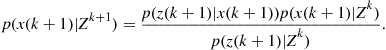 (15.32)
The above recursive propagation of the posterior density is only a conceptual solution. Analytical formulas of the posterior density exist only in a restrictive set of cases.
3.15.3.1 Kalman filter
The Kalman filter assumes that the state and measurement models are linear, i.e., ![]() . Also, in the Kalman filter, the initial state error and all the noises entering into the system are assumed to be Gaussian, i.e.,
. Also, in the Kalman filter, the initial state error and all the noises entering into the system are assumed to be Gaussian, i.e., ![]() is white and Gaussian with zero mean and covariance
is white and Gaussian with zero mean and covariance ![]() , and
, and ![]() is white and Gaussian with zero mean and covariance
is white and Gaussian with zero mean and covariance ![]() . Under the above assumptions, if
. Under the above assumptions, if ![]() is Gaussian, it can be proved that
is Gaussian, it can be proved that ![]() is also Gaussian, which can be parameterized by a mean and covariance [10].
is also Gaussian, which can be parameterized by a mean and covariance [10].
The Kalman filter algorithm consists of the following recursive relationship [10]:
![]() (15.33)
(15.33)
![]() (15.34)
(15.34)
![]() (15.35)
(15.35)
![]() (15.36)
(15.36)
![]() (15.37)
(15.37)
![]() (15.38)
(15.38)
where
![]() (15.39)
(15.39)
The Kalman filter is the optimal solution to the tracking problem if the above assumptions hold because it provides the posterior probability density of targets state.
3.15.3.2 Extended Kalman filter (EKF)
While the Kalman filter assumes linearity, most of the real world problems are nonlinear. The extended Kalman filter is a suboptimal state estimation algorithm for nonlinear systems. In EKF, local linearizations of the equations are used to describe the nonlinearity,
![]() (15.40)
(15.40)
![]() (15.41)
(15.41)
The EKF assumes that ![]() can be approximated by a Gaussian. Then the equations of the Kalman filter can be used with this approximation and the linearized functions, except the state and measurement prediction are performed using the original nonlinear functions
can be approximated by a Gaussian. Then the equations of the Kalman filter can be used with this approximation and the linearized functions, except the state and measurement prediction are performed using the original nonlinear functions
![]() (15.42)
(15.42)
![]() (15.43)
(15.43)
The above is a first-order EKF based on the first-order series expansion of the nonlinearities. There are several error reduction methods to improve the performance of the EKF [10]. One of them is using the second-order series expansion of the nonlinearities, i.e., higher-order EKFs, but the additional complexity and little or no benefit has prohibited its widespread use. For continuous-time nonlinear systems, numerical integration on the continuous-time stochastic differential equation of the state from ![]() to
to ![]() can be used to obtain a better predicted state. The third approach to improve the EKF is using an iteration to compute the updated state as a maximum a posterior (MAP) estimate, rather than an approximate conditional mean. This type of EKF is called the Iterated extended Kalman filter (IEKF). The iteration used by the IEKF amounts to relinearize the measurement equation around the updated state rather than relying only on the predicted state. If the measurement model fully observes the state, then the IEKF is able to handle the non-linear measurement model better than the EKF [61].
can be used to obtain a better predicted state. The third approach to improve the EKF is using an iteration to compute the updated state as a maximum a posterior (MAP) estimate, rather than an approximate conditional mean. This type of EKF is called the Iterated extended Kalman filter (IEKF). The iteration used by the IEKF amounts to relinearize the measurement equation around the updated state rather than relying only on the predicted state. If the measurement model fully observes the state, then the IEKF is able to handle the non-linear measurement model better than the EKF [61].
3.15.3.3 Unscented Kalman filter (UKF)
When the state transition and observation models are highly nonlinear, the EKF may perform poorly. The unscented Kalman filter does not approximate the nonlinear functions of state and measurement models as required by the EKF. Instead, the UKF uses a deterministic sampling technique known as the unscented transform to pick a minimal set of sample points called sigma points around the mean. Here, the propagated mean and covariance are calculated from the transformed samples [52]. In some UKF implementations, the state random variable is augmented as the concatenation of the original state and noise variables [123]. The steps of UKF are described below.
3.15.3.3.1 Sigma point generation
The state vector ![]() with mean
with mean ![]() and covariance
and covariance ![]() is approximated by
is approximated by ![]() weighted sigma points, where
weighted sigma points, where ![]() is the dimension of the state vector, as
is the dimension of the state vector, as
![]() (15.44)
(15.44)
![]() (15.45)
(15.45)
![]() (15.46)
(15.46)
where ![]() is the weight associated with the ith point,
is the weight associated with the ith point, ![]() is a scaling parameter,
is a scaling parameter, ![]() , and
, and ![]() is the ith row or column of the matrix square root of
is the ith row or column of the matrix square root of ![]() .
.
3.15.3.3.2 Recursion
1. Find the predicted target state ![]() and corresponding covariance
and corresponding covariance ![]() :
:
a. Transform the Sigma points using the system model
![]() (15.47)
(15.47)
 (15.48)
c. Find the predicted covariance
 (15.49)
2. Find the predicted measurement ![]() and the corresponding covariance
and the corresponding covariance ![]() :
:
a. Regenerate the Sigma points ![]() using the mean
using the mean ![]() and covariance
and covariance ![]() in order to incorporate the effect of
in order to incorporate the effect of ![]() . If
. If ![]() is zero, the resulting
is zero, the resulting ![]() will be the same as in (15.47). If the process noise is correlated with the state, then the noise vector must be stacked with the state vector
will be the same as in (15.47). If the process noise is correlated with the state, then the noise vector must be stacked with the state vector ![]() before generating the sigma points [52].
before generating the sigma points [52].
b. Find the predicted measurement mean ![]()
 (15.50)
where
![]() (15.51)
(15.51)
c. Find the innovation covariance ![]() and gain
and gain ![]()
 (15.52)
3. Update the state ![]() and corresponding covariance
and corresponding covariance ![]() using (15.37) and (15.38), respectively.
using (15.37) and (15.38), respectively.
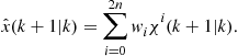
3.15.3.4 Particle filter
If the true density is substantially non-Gaussian, then a Gaussian model as in the case of the Kalman filter will not yield accurate estimates. In such cases, particle filters will yield an improvement in performance in comparison to the EKF or UKF. The particle filter provides a mechanism for representing the density, ![]() of the state vector
of the state vector ![]() at time epoch
at time epoch ![]() as a set of random samples
as a set of random samples ![]() , with associated weights
, with associated weights ![]() . That is, the particle filter attempts to represent an arbitrary density function using a finite number of points, instead of a pair of mean vector and covariance matrix that is sufficient for Gaussian distributions. Several variations of particle filters are available and the reader is referred to [3] for detailed description. The Sampling Importance Resampling (SIR) type particle filter, which is arguably the most common technique to implement particle filters, is discussed below. In general, the particles are sampled either from the prior density or likelihood function. Taking the prior as the importance density, the method of SIR is used to produce a set of equally weighted particles that approximates
. That is, the particle filter attempts to represent an arbitrary density function using a finite number of points, instead of a pair of mean vector and covariance matrix that is sufficient for Gaussian distributions. Several variations of particle filters are available and the reader is referred to [3] for detailed description. The Sampling Importance Resampling (SIR) type particle filter, which is arguably the most common technique to implement particle filters, is discussed below. In general, the particles are sampled either from the prior density or likelihood function. Taking the prior as the importance density, the method of SIR is used to produce a set of equally weighted particles that approximates ![]() , i.e.,
, i.e.,
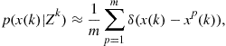 (15.53)
where ![]() is the Dirac Delta function. The prediction and update steps of the particle filter recursion are given below.
is the Dirac Delta function. The prediction and update steps of the particle filter recursion are given below.
Prediction: Take each existing sample, ![]() and generate a sample
and generate a sample ![]() , using the system model. The set
, using the system model. The set ![]() provides an approximation of the prior,
provides an approximation of the prior, ![]() , at time
, at time ![]() .
.
Update: At each measurement epoch, to account for the fact that the samples, ![]() are not drawn from
are not drawn from ![]() , the weights are modified using the principle of importance sampling. When using the prior as the importance density, it can be shown that the weights are given by
, the weights are modified using the principle of importance sampling. When using the prior as the importance density, it can be shown that the weights are given by
![]() (15.54)
(15.54)
A common problem with the above recursion is the degeneracy phenomenon, whereby the particle set quickly collapses to just a single particle. To overcome this problem a regularization can be imposed via reselection as follows.
Reselection: Resample (with replacement) from ![]() , using the weights,
, using the weights, ![]() , to generate a new sample,
, to generate a new sample, ![]() , then set
, then set ![]() for
for ![]() .
.
The mean of the posterior distribution is used to estimate, ![]() of the target state,
of the target state, ![]() , i.e.,
, i.e.,
 (15.55)
The accuracy of the particle filter based estimate (15.53) depends on the number of particles employed. A more accurate state estimates can be obtained at the expense of extra computation. The extension of particle filters allows them to be applicable to multitarget tracking problems [60].
3.15.3.5 Interacting multiple-model estimator
Tracking maneuvering targets is a very important task for almost all practical systems. Several schemes and methods have been proposed to track maneuvering targets [69–73]. One of widely used method is the Multiple Mode (MM) approach [10]. In MM approach, the target system is assumed to follow one of predetermined models (or mods) and a number of filters operate in parallel. Thus, the system has both continuous uncertainties brought by the noise, and discrete uncertainties brought by the model uncertainty. Starting from the prior distribution of the target state and the prior probability that the system is in a particular mode, the goal of the MM approach is to obtain the posterior distribution of the target state and posterior mode probability.
Depending on whether mode jumping is allowed, there are static MM estimator and dynamic MM estimator. In static MM algorithms, it is assumed that there is no model switching from one mode to another during the whole estimation process and this assumption is not realistic for many real scenarios. On the other hand, in dynamic MM algorithms, the target is allowed to switch from one mode to another according to a Markov chain. Optimal dynamic MM estimator is infeasible since it needs to carry all the mode sequence hypotheses and the total number of the mode sequence hypotheses increases exponentially with time. To get a feasible dynamic MM suboptimal estimator, the mode sequences that only differ in “older” modes are combined and the mode sequences are kept to depth ![]() in the Generalized Pseudo-Bayesian (GPB) approaches [9,10]. A GPB algorithm of depth
in the Generalized Pseudo-Bayesian (GPB) approaches [9,10]. A GPB algorithm of depth ![]() (
(![]() ) requires
) requires ![]() filters in its bank, where
filters in its bank, where ![]() is the number of models.
is the number of models.
The Interacting Multiple Model (IMM) estimator [9,10,15,16], which mixes the mode sequence hypotheses with depth ![]() at the beginning of each filtering cycle, requires only
at the beginning of each filtering cycle, requires only ![]() number of filters to operate in parallel, (i.e., same as
number of filters to operate in parallel, (i.e., same as ![]() estimator) but is able to perform nearly as well as
estimator) but is able to perform nearly as well as ![]() . Thus, the IMM estimator is very cost-efficient. The main contributor for the cost-efficiency of the IMM estimator is the “mixing/interaction” between its “mode-matched” base state filtering modules at the beginning of each cycle. It has been shown in [7], the same feature is exactly what the IMM has in common with the optimal estimator for dynamic MM systems. Besides its cost-efficiency, another advantage of the IMM estimator is that it does not require maneuver detection decision as in the case of Variable State Dimension (VSD) filter [10] algorithms and undergoes a soft switching between models based on the updated mode probabilities.
. Thus, the IMM estimator is very cost-efficient. The main contributor for the cost-efficiency of the IMM estimator is the “mixing/interaction” between its “mode-matched” base state filtering modules at the beginning of each cycle. It has been shown in [7], the same feature is exactly what the IMM has in common with the optimal estimator for dynamic MM systems. Besides its cost-efficiency, another advantage of the IMM estimator is that it does not require maneuver detection decision as in the case of Variable State Dimension (VSD) filter [10] algorithms and undergoes a soft switching between models based on the updated mode probabilities.
3.15.3.5.1 Modeling assumptions in dynamic multiple model approach
Base state model:
![]() (15.56)
(15.56)
![]() (15.57)
(15.57)
where ![]() denotes the mode in effect during the sampling period ending at
denotes the mode in effect during the sampling period ending at ![]() .
.
Mode (“model state”)—among the possible ![]() modes:
modes:
![]() (15.58)
(15.58)
The structure of the system and/or the statistics of the noises can differ from mode to mode:
![]() (15.59)
(15.59)
![]() (15.60)
(15.60)
Mode jump process: Markov chain with known transition probabilities
![]() (15.61)
(15.61)
3.15.3.5.2 The IMM estimation algorithm
• Interaction: Mixing of the previous cycle mode-conditioned state estimates and covariance, using the mixing probabilities ![]() , to initialize the current cycle of each mode-conditioned filter. For filter
, to initialize the current cycle of each mode-conditioned filter. For filter ![]() , there is:
, there is:
![]() (15.62)
(15.62)
 (15.63)
where
![]() (15.64)
(15.64)
![]() (15.65)
(15.65)
• Mode-conditioned filtering: Calculation of the state estimates and covariances conditioned on a mode being in effect. The KF matched to ![]() (filter
(filter ![]() ) uses
) uses ![]() to yield
to yield ![]() and
and ![]() . Likelihood function corresponding to filter
. Likelihood function corresponding to filter ![]() is
is ![]() .
.
• Probability evaluation: Computation of the mixing and the updated mode probabilities. For the mode probabilities of the jth mode (![]() )
)
![]() (15.66)
(15.66)
 (15.67)
• Overall state estimate and covariance (for output only): Combination of the latest mode-conditioned state estimates and covariances
 (15.68)
 (15.69)
The IMM estimation algorithm has a modular structure.
For non-maneuvering targets, unnecessarily using multiple-model algorithms is not optimal because it might diminish the performance level of the tracker and increase the computational load. A multiple-model approach is only necessary for targets with high maneuverability. Typically, the decision to use a multiple-model estimator should be based on the maneuvering index [10], which quantifies the maneuverability of the target in terms of the process noise, sensor measurement noise and sensor revisit interval. In [56], a study was presented to compare the IMM estimator with the Kalman filter based on the maneuvering index.
3.15.4 Filter initialization
Track initiation is an essential component of all tracking algorithms. Two major types of initialization techniques, namely, the Single-Point (SP) method and the Two-Point-Difference (TPD) method, are commonly used in multisensor-multitarget tracking applications [9,10,84].
3.15.4.1 Single-point track initialization
In SP track initialization, every detection (measurement), which is unassociated to any track, is an “initiator.” The unassociated measurement is first converted into Cartesian space through the unbiased conversion method [10] and then a tentative track is declared. In SP algorithm, the position component of the tentative track is initialized using the position component of the converted measurement and the velocity components is set to zero. To compensate the zero velocity assumption made for the tentative track, when initializing the covariance matrix of the tentative track, the maximum possible speed of the target is often used as the standard deviation of the velocity component of the tentative track. For the position component, the variance of the converted measurement is used. Furthermore, for the newly declared tentative track, its velocity and position along different coordinates are usually assumed to be independent. A Kalman filter is then used for subsequent processing of the tentative track.
3.15.4.2 Two-point difference track initialization
In TPD track initialization, every unassociated detection (measurement) is also an “initiator,” but does not immediately yield a tentative track. At the sampling time (scan or frame) following the detection of an initiator, a gate is set up around the initiator based on the assumed maximum and minimum target speed as well as the measurement noise intensities. Thus, it is reasonable to assume that if the initiator is from a target, then the measurement from that target in the second scan (if detected) will fall inside the gate with nearly unity probability. A tentative track will be declared only if there is at least one detection falling in the gate. Since now each tentative track has two measurements, a straight line extrapolation is used to obtain its speed and the covariance matrix. A Kalman filter is then used for the subsequent processing.
3.15.4.3 Issues related to track initialization
It has been demonstrated numerically that the SP method has a smaller mean square error matrix than the TPD method for a 3D radar target tracking problem. Also, it has been analytically shown that, if the process noise approaches zero and the maximum speed of a target used to initialize the velocity variance approaches infinity, then the SP algorithm reduces to the TPD algorithm [84].
In many multi-sensor multitarget tracking algorithms, the track initialization and the track maintenance phases are treated as two independent (and consecutive) stages. However, in a real tracking problems, targets can enter and leave the surveillance region at any time. As a result, track initiation has to be considered at every sampling time. That is, track initialization occurs even after the first few scan. Similarly, the fact that track maintenance stage has been activated does not obviate the need for further track initiations. Both have to be carried out simultaneously throughout the entire tracking interval. Because of this, the track initialization module needs to take into account the number, states and qualities of the established tracks being retained by the track maintenance module. Otherwise, spurious tracks and track seduction will ensue, damaging the overall quality of the tracker [42].
3.15.5 Data association
In Section 3.15.3, it has been implicitly assumed that there is no measurement origin ambiguity. However, the crux of the multitarget problem is to carry out the association process for measurements whose origins are uncertain due to
• random false alarms in the detection process,
• clutter due to spurious reflectors or radiators near the target of interest,
Furthermore, the probability of obtaining a measurement from a target—the target detection probability—is usually less than unity.
Data association problems may be categorized according to the pairs of information that are associated together:
• measurement-to-track association—track maintenance or updating,
• measurement-to-measurement association—parallel updating for centralized tracking,
• track-to-track association—track fusion (for distributed or decentralized tracking).
In this subsection, measurement-to-track association and measurement-to-measurement association techniques are discussed. The track-to-track association is discussed in Section 3.15.9.
3.15.5.0.1 Measurement-to-track association
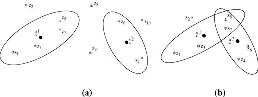
A multidimensional gate is set up in the measurement space around the predicted measurement in order to avoid searching for the measurement from the target of interest in the entire measurement space. A measurement in the gate, while not guaranteed to have originated from the target the gate pertains to, is a valid association candidate. Thus the name validation region or association region. If there is more than one measurement in the gate, this leads to an association uncertainty.
Figure 15.1a and b illustrates the gating for two well-separated and closely-spaced targets respectively. In the figures, “![]() ” indicates the expected measurement and the “
” indicates the expected measurement and the “![]() ” indicates the received measurement.
” indicates the received measurement.
If the true measurement conditioned on the past is normally (Gaussian) distributed with its probability density function given by
![]() (15.70)
(15.70)
then the true measurement will be in the following region:
![]() (15.71)
(15.71)
with probability determined by the gate threshold ![]() . The region defined by (15.71) is called gate or validation region.
. The region defined by (15.71) is called gate or validation region.
Some well-known approaches for data association in the presence of well-separated targets, where no measurement origin uncertainties exist are discussed below.
Nearest Neighbor (NN): This is the simplest possible approach and uses the measurement nearest to the predicted measurement, assuming that the nearest one is the correct one. The nearest measurement to the predicted measurement is determined according to the distance measure (norm of the innovation squared),
![]() (15.72)
(15.72)
Strongest Neighbor (SN): Select the strongest measurement (in terms of signal intensity) among the validated ones—this assumes that signal intensity information is available.
2-D Assignment: This technique is also known as the Global Nearest Neighbor (GNN) method. The fundamental idea behind 2-D assignment is that the measurements from the scan list ![]() at time
at time ![]() are deemed to have come from the tracks in list
are deemed to have come from the tracks in list ![]() at time
at time ![]() . To find the best match between
. To find the best match between ![]() and
and ![]() , a constrained global optimization problem has to be solved. The optimization is carried out to minimize the “cost” of associating the measurements in
, a constrained global optimization problem has to be solved. The optimization is carried out to minimize the “cost” of associating the measurements in ![]() to tracks predicted from
to tracks predicted from ![]() .
.
To present the 2-D assignment, define a binary assignment variable ![]() such that
such that
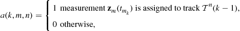 (15.73)
where ![]() is the time stamp of the mth measurement from scan or frame
is the time stamp of the mth measurement from scan or frame ![]() .
.
A set of complete assignments, which consists of the associations of all the measurements in ![]() and the tracks in
and the tracks in ![]() , is denoted by
, is denoted by ![]() , i.e.,
, i.e.,
![]() (15.74)
(15.74)
where ![]() and
and ![]() are the cardinalities of the measurement and track sets, respectively. The indices
are the cardinalities of the measurement and track sets, respectively. The indices ![]() and
and ![]() correspond to the non-existent (or “dummy”) measurement and track. The “dummy” notation is used to formulate the assignment problem in a uniform manner, where the non-association possibilities are also considered, making it computer-solvable.
correspond to the non-existent (or “dummy”) measurement and track. The “dummy” notation is used to formulate the assignment problem in a uniform manner, where the non-association possibilities are also considered, making it computer-solvable.
The objective of the assignment is to find the optimal assignment ![]() , which minimizes the global cost of association
, which minimizes the global cost of association
 (15.75)
where ![]() is the cost of the assignment
is the cost of the assignment ![]() . That is,
. That is,
![]() (15.76)
(15.76)
The costs ![]() are the negative of the logarithm of the dimensionless likelihood ratio of the measurement-to-track associations, namely,
are the negative of the logarithm of the dimensionless likelihood ratio of the measurement-to-track associations, namely,
![]() (15.77)
(15.77)
where
 (15.78)
are the following likelihood ratios:
1. that measurement ![]() came from track
came from track ![]() for
for ![]() with the association likelihood function being the probability density function of the corresponding innovation,
with the association likelihood function being the probability density function of the corresponding innovation, ![]() versus from an extraneous source whose spatial density is
versus from an extraneous source whose spatial density is ![]() ,
,
2. that measurement ![]() came from none of the tracks (i.e., from the dummy track
came from none of the tracks (i.e., from the dummy track ![]() ) versus from an extraneous source. Note that, if measurement
) versus from an extraneous source. Note that, if measurement ![]() came from none of the tracks, then that measurement must be generated by an extraneous source, Thus, the likelihood ratio must be unity in this case,
came from none of the tracks, then that measurement must be generated by an extraneous source, Thus, the likelihood ratio must be unity in this case,
3. that the measurement from track ![]() is not in
is not in ![]() , i.e., track
, i.e., track ![]() is associated with the dummy measurement—the cost of not associating any measurement to a track amounts to the miss probability
is associated with the dummy measurement—the cost of not associating any measurement to a track amounts to the miss probability ![]() , where the nominal target detection probability is denoted by
, where the nominal target detection probability is denoted by ![]() .
.
The 2-D assignment is subject to the following constraints.Validation: A measurement is assigned only to one of the tracks that validated it.One-to-one constraint: Each track is assigned at most one measurement. The only exception is the dummy track ![]() , which can be associated with any number of measurements. Similarly, a measurement is assigned to at most one track. The dummy measurement
, which can be associated with any number of measurements. Similarly, a measurement is assigned to at most one track. The dummy measurement ![]() can be assigned to multiple tracks.Non-empty association: The association cannot be empty, i.e., the dummy measurement cannot be assigned to the dummy track.
can be assigned to multiple tracks.Non-empty association: The association cannot be empty, i.e., the dummy measurement cannot be assigned to the dummy track.
The modified auction algorithm can solve the above constrained optimization problem and that algorithm runs in quasi-polynomial time [94,95].
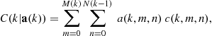
Multidimensional (S-D) Assignments: In 2-D assignment only the latest scan is used and information about target evolution through multiple scans is lost. Also it is not possible to change an association later in light of subsequent measurements. A data-association algorithm may perform better when a number of past scans are utilized. This corresponds to multidimensional assignment for data association. In S-D assignment the latest ![]() scans of measurements are associated with the established track list (from time
scans of measurements are associated with the established track list (from time ![]() , where
, where ![]() is the current time, i.e., with a sliding window of time depth
is the current time, i.e., with a sliding window of time depth ![]() ) in order to update the tracks.
) in order to update the tracks.
Similarly to the 2-D assignment, define a binary assignment variable ![]() such that
such that
 (15.79)
which is the general version of (15.73). The cost associated with (15.79) is denoted as
![]() (15.80)
(15.80)
and ![]() is the likelihood ratio that the S-1-tuple of measurements, which is given by
is the likelihood ratio that the S-1-tuple of measurements, which is given by ![]() , originated from the target represented by track
, originated from the target represented by track ![]() versus some measurements
versus some measurements ![]() being extraneous.
being extraneous.
The objective of the S-D assignment is to find the S-tuples of measurement-to-track associations ![]() , which minimize the global cost of association given by
, which minimize the global cost of association given by
 (15.81)
where ![]() is the number of measurements in scan
is the number of measurements in scan ![]() and
and ![]() is the complete set of associations analogous to that defined in (15.74) for the 2-D assignment. The association likelihoods are given by
is the complete set of associations analogous to that defined in (15.74) for the 2-D assignment. The association likelihoods are given by
 (15.82)
where ![]() is a binary function such that
is a binary function such that
 (15.83)
and ![]() is the filter-calculated innovation pdf if the (kinematic) measurement
is the filter-calculated innovation pdf if the (kinematic) measurement ![]() is associated with track
is associated with track ![]() continued with the (kinematic) measurements
continued with the (kinematic) measurements ![]() .
.
The association costs are given to the generalized S-D assignment algorithm, which uses Lagrangian relaxation, as described in [32,95] to solve the assignment problem in quasi-polynomial time. The feasibility constraints are similar to those from the 2-D assignment.
3.15.5.0.2 Measurement-to-measurement association
Measurement-to-measurement association is the most important step in the parallel updating scheme for the centralized tracking. Without any major modification, multidimensional (S-D) Assignments and 2-D Assignment technique are commonly used for measurement-to-measurement association. A good example of using S-D assignment technique to solve the measurement-to-measurement association problem in a multisensor-multitarget tracking problem is given in [9].
3.15.6 Multitarget tracking algorithms
Three widely used multitarget tracking algorithms, namely, the Probabilistic Data Association (PDA) and Joint Probabilistic Data Association (JPDA) algorithm, the Multiple Hypothesis Tracker (MHT) algorithm, and the Probability Hypothesis Density (PHD) algorithm, are discussed in this section.
3.15.6.1 Probabilistic data association (PDA) and joint probabilistic data association (JPDA)
PDA algorithm is a Bayesian approach that probabilistically associates all the validated measurements to the target of interest [9]. The state update equation of the PDA filter is
![]() (15.84)
(15.84)
where
 (15.85)
![]() (15.86)
(15.86)
![]() is the number of validated measurements and
is the number of validated measurements and
![]() (15.87)
(15.87)
is the conditional probability of the event that the ith validated measurement is correct.
The covariance associated with the updated state is
![]() (15.88)
(15.88)
where ![]() is the conditional probability of the event that none of the measurements is correct and the covariance of the state updated with the correct measurement is
is the conditional probability of the event that none of the measurements is correct and the covariance of the state updated with the correct measurement is
![]() (15.89)
(15.89)
In equation (15.89), the gain matrix ![]() and the innovation matrix
and the innovation matrix ![]() are calculated using the standard Kalman filter equation (15.36), (15.39). The spread of the innovations term in (15.88) is
are calculated using the standard Kalman filter equation (15.36), (15.39). The spread of the innovations term in (15.88) is
 (15.90)
The association of measurements in a multitarget environment with closely-spaced targets must be done while simultaneously considering all the targets. Thus, the Joint Probabilistic Data Association (JPDA) is proposed as an extension of the PDA method to handle the scenario with closely-spaced targets [9]. For a known number of targets, JPDA evaluates the measurement-to-target association events probabilities (for the latest set of measurements) and combines them into the corresponding state estimates.
The JPDA algorithm includes the following steps:
• A validation matrix that indicates all the possible sources of each measurement is set up.
• From the validation matrix, all the feasible joint association events are constructed by the JPDA tracker according to the following two rules:
• One measurement must be originated from one target or a false alarm.
• One target can only generate one measurement at most.
• The probabilities of these joint events are evaluated according to the following assumptions:
• Target-originated measurements are Gaussian distributed around the predicted location of the corresponding target’s measurement.
• False alarms are distributed in the surveillance region according to a Poisson point process model.
• Marginal (individual measurement-to-target) association probabilities are obtained from the joint association probabilities.
• The target states are estimated by separate (uncoupled) PDA filters using these marginal probabilities.
An extension of the PDA algorithm, the Integrated Probabilistic Data Association (IPDA) algorithm is proposed in [85]. The main idea behind IPDA tracker is to introduce the track existence probability, a measure of the quality of the track, to the PDA algorithm. Like PDA tracker, IPDA track can only be used to track well-separated targets in clutter. To handle the multitarget environment with closely-spaced targets, the Joint Integrated Probabilistic Data Association (JIPDA) tracker is proposed in [86], which is actually a JPDA with the track existence probability.
3.15.6.2 Multiple Hypothesis Tracker (MHT)
Multiple Hypothesis Tracking (MHT) is an efficient algorithm for tracking multitargets in a cluttered environment. The algorithm is capable of initiating tracks, accounting false or missing reports, and processing sets of dependent reports. As each measurement is received, probabilities are calculated for the hypotheses that the measurement came from previously existing target, or from a new target, or that the measurement is a false alarm. Target states are estimated from each such data-association hypothesis with a certain filter (e.g., Kalman Filter). As more measurements are received, the probabilities of joint hypotheses are calculated recursively using all available information such as the density of unknown target ![]() , the density of false targets
, the density of false targets ![]() and the probability of detection
and the probability of detection ![]() . This branching technique allows the correlation of a measurement with its source based on subsequent, as well as previous, data. To keep the number of hypotheses reasonable, unlikely hypotheses are eliminated and hypotheses with similar target estimates are combined. To minimize computational requirements, clustering and pruning techniques are embedded in the MHT tracker. Note that MHT strictly follows the one-to-one assumption between measurements and targets. There are two types of implementation for MHT, the hypothesis-oriented MHT (HOMHT), which is also known as the measurement-oriented MHT (MOMHT), and the track-oriented MHT (TOMHT).
. This branching technique allows the correlation of a measurement with its source based on subsequent, as well as previous, data. To keep the number of hypotheses reasonable, unlikely hypotheses are eliminated and hypotheses with similar target estimates are combined. To minimize computational requirements, clustering and pruning techniques are embedded in the MHT tracker. Note that MHT strictly follows the one-to-one assumption between measurements and targets. There are two types of implementation for MHT, the hypothesis-oriented MHT (HOMHT), which is also known as the measurement-oriented MHT (MOMHT), and the track-oriented MHT (TOMHT).
3.15.6.2.1 Hypothesis-oriented MHT (HOMHT)
In HOMHT, hypotheses are composed of sets of compatible tracks. Multiple tracks are compatible if they have no measurement in common. At every scan, each hypothesis carried over from the previous scan (i.e., parent hypothesis) is expanded into a set of new hypotheses (i.e., offspring hypothesis) by considering all possible track-to-measurement associations for the tracks within the parent hypothesis [9]. The HOMHT includes the following steps:
• Initialization: The measurements received at the first scan ![]() have two possible origination: (1) new target with probability
have two possible origination: (1) new target with probability ![]() ; (2) false alarm with probability
; (2) false alarm with probability ![]() . Therefore, the total number of possible hypotheses is
. Therefore, the total number of possible hypotheses is ![]() where
where ![]() is the number of measurements received at scan
is the number of measurements received at scan ![]() . The probability of each hypothesis is proportional to
. The probability of each hypothesis is proportional to
![]() (15.91)
(15.91)
where ![]() and
and ![]() denote the number of measurements that are assigned as new targets and the number of measurements that are assigned as false alarms give the jth valid hypothesis
denote the number of measurements that are assigned as new targets and the number of measurements that are assigned as false alarms give the jth valid hypothesis ![]() . Then, select the top
. Then, select the top ![]() hypotheses based on their probabilities
hypotheses based on their probabilities ![]() . These
. These ![]() hypotheses
hypotheses ![]() are parent hypotheses for the next scan, and their probabilities are normalized at the end of this scan.
are parent hypotheses for the next scan, and their probabilities are normalized at the end of this scan.
• Update of hypotheses: In this step, every parent hypothesis will be used to generate a set of offspring hypotheses. The collection of all the offspring hypotheses forms the current set of hypotheses. Then, top ![]() hypotheses will be selected from the current set of hypotheses, and their probabilities will be normalized.
hypotheses will be selected from the current set of hypotheses, and their probabilities will be normalized.
• Prune hypotheses: It is infeasible to keep all the hypotheses because the number of hypotheses grows exponentially. Several pruning techniques are embedded to the HOMHT tracker to maintain the number of hypotheses in a suitable level. The first pruning method removes hypothesis whose probability is less than a predefined threshold ![]() . The second pruning method keeps only the top
. The second pruning method keeps only the top ![]() hypotheses with the greatest probabilities. The third method discards the set of hypotheses with the smallest probabilities such that the total probability of discarded hypotheses does not exceed a user defined threshold
hypotheses with the greatest probabilities. The third method discards the set of hypotheses with the smallest probabilities such that the total probability of discarded hypotheses does not exceed a user defined threshold ![]() . For example, the probabilities of all the current hypotheses are
. For example, the probabilities of all the current hypotheses are ![]() . Assume that
. Assume that ![]() and
and ![]() . Then, the third method removes the
. Then, the third method removes the ![]() th to nth hypotheses where
th to nth hypotheses where ![]() and
and ![]() .
.
• Track management: In HOMHT tracker, two kinds of track management systems are available. The first is based on ![]() logic and the second relies on track qualities. Note that, the HOMHT tracker does not probabilistically combine the update states, which are calculated conditioning on the measurement-to-track association events. Thus the equations that used in JIPDA tracker can not be applied here. One method to compute the track quality in the MHT framework is proposed in [88].
logic and the second relies on track qualities. Note that, the HOMHT tracker does not probabilistically combine the update states, which are calculated conditioning on the measurement-to-track association events. Thus the equations that used in JIPDA tracker can not be applied here. One method to compute the track quality in the MHT framework is proposed in [88].
• Find the best hypothesis and output: The last step of a HOMHT loop for a scan is to find the best current hypothesis and then output it to the user.
3.15.6.2.2 Track oriented MHT (TOMHT)
The track-oriented MHT constructs a target tree for each potential (or postulated) target according to the measurements, and the branches represent the different measurements with which the target may be associated. A trace of successive branches from the root to a leaf of the tree represents a potential measurement history generated by the target. Conventionally, the target trees are referred to as track hypotheses, and a collection of compatible tracks is referred to as global hypothesis. Unlike the HOMHT in which three possible originalities of measurement are considered, usually the TOMHT treats a measurement as either originated from an existing target or a new one [13]. The TOMHT includes the following steps:
• Initialize tree: The target trees are initialized on the receipt of the first set of measurements. The root of each tree is a measurement.
• Build tree: In this step, the set of trees of previous scan are updated. More specifically, (1) the depth of each previous tree is increased by one and each branch grows to several new branches to account for all possible target-to-measurement associations; (2) each measurement also is used to initiate a new target tree where the measurement is the root of the tree. In addition, the compatibility relation has to be updated in order to find the global hypothesis.
• Track management: The track management techniques used for TOMHT are the same as that used for HOMHT.
• Track level pruning: The purpose of this step is to remove the branches of low probabilities so that the computation load for finding the global hypothesis is remained in a reasonable level. Two pruning methods can be embedded into the HOMHT: (1) limit the number of branches per tree below ![]() , which is defined by user as the maximum number of branches per tree; (2) discard the branches whose probability is lower than a predefined threshold
, which is defined by user as the maximum number of branches per tree; (2) discard the branches whose probability is lower than a predefined threshold ![]() .
.
• Find clusters: All the branches, i.e., the node or potential track, belong to the same target tree are within the same cluster because they share the same root. Therefore, the clustering procedure for TOMHT is done in the tree-to-measurement level. The algorithm and code for HOMHT clustering can be reused for TOMHT by just replacing the track by tree and measurement associated with track by measurements associated with target tree.
• Find global hypothesis: This step is used to find the best global hypothesis, which is a collection of compatible trees from all the target trees. Enumeration is the basic method for finding the best global hypothesis. In enumeration method, all valid global hypotheses are constructed and then the best one is chosen according to the costs of hypotheses. However, the total number of valid global hypotheses grows exponentially with respect to the number of trees. For example, assume that ![]() trees exist and there are
trees exist and there are ![]() branches for each tree. Then, the total number of global hypotheses is
branches for each tree. Then, the total number of global hypotheses is ![]() . Although some of the invalid hypotheses will be removed from this
. Although some of the invalid hypotheses will be removed from this ![]() hypotheses, the remaining part is still a large amount. Therefore, the pruning method must be used to limit the number of valid hypotheses and then an approximate best global hypothesis is found.
hypotheses, the remaining part is still a large amount. Therefore, the pruning method must be used to limit the number of valid hypotheses and then an approximate best global hypothesis is found.
Due to the requirement of node compatibility (or track compatibility), one and only one branch must be selected per tree to form a possible valid global hypothesis. Note that the selection of dummy node means no track is selected from this tree in the global hypothesis.
3.15.6.3 Probability hypothesis density (PHD) method
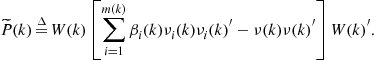
In tracking multiple targets, if the number of targets is unknown and varying with time, it is not possible to compare states with different dimensions using ordinary Bayesian statistics. However, the problem can be addressed using Finite Set Statistics (FISST) [75] to incorporate comparisons of states of different dimensions. FISST facilitates the construction of “multitarget densities” from multiple target transition functions into computing set derivatives of belief-mass functions [75], which makes it possible to combine states of different dimensions. The main practical difficulty with this approach is that the dimension of state space becomes large when many targets are present, which increases the computational load exponentially with the number of targets. Since the PHD is defined over the state space of one target in contrast to the full posterior distribution, which is defined over the state space of all the targets, the computation cost of propagating the PHD over time is much lower than propagating the full posterior density. A comparison in terms of computation and estimation accuracy of multitarget filtering using FISST particle filter and PHD particle filter is given in [112].
Assume a sensor has monitored an area since time ![]() and at time
and at time ![]() , the measurement set
, the measurement set ![]() is provided by that sensor. From time
is provided by that sensor. From time ![]() to time
to time ![]() , the union of all available measurement sets from that sensor are
, the union of all available measurement sets from that sensor are ![]() . By definition, the PHD
. By definition, the PHD ![]() , with argument single-target state vector
, with argument single-target state vector ![]() and all available measurement sets up to time step
and all available measurement sets up to time step ![]() , is the density whose integral on any region
, is the density whose integral on any region ![]() of the state space is the expected number of targets
of the state space is the expected number of targets ![]() contained in
contained in ![]() . That is,
. That is,
![]() (15.92)
(15.92)
Since this property uniquely characterizes the PHD and since the first order statistical moment of the full target posterior distribution possesses this property, the first order statistical moment of the full target posterior is indeed the PHD. The first moment of the full target posterior or the PHD, given all the measurement sets ![]() up to time step
up to time step ![]() , is given by [76]
, is given by [76]
![]() (15.93)
(15.93)
where ![]() is the multitarget state. The approximate expected target states are given by the local maxima of the PHD. The following section demonstrates the prediction and update steps of one cycle of the PHD filter.
is the multitarget state. The approximate expected target states are given by the local maxima of the PHD. The following section demonstrates the prediction and update steps of one cycle of the PHD filter.
Prediction: In a general scenario of interest, there are target disappearances, target spawning and entry of new targets. We denote the probability that a target with state ![]() at time step
at time step ![]() will survive at time step
will survive at time step ![]() by
by ![]() , the PHD of spawned targets at time step
, the PHD of spawned targets at time step ![]() from a target with state
from a target with state ![]() by
by ![]() and the PHD of newborn spontaneous targets at time step
and the PHD of newborn spontaneous targets at time step ![]() by
by ![]() . Then, the predicted PHD is given by
. Then, the predicted PHD is given by
 (15.94)
where ![]() denotes the single-target Markov transition density. The prediction Eq. (15.94) is lossless since there are no approximations.
denotes the single-target Markov transition density. The prediction Eq. (15.94) is lossless since there are no approximations.
Update: The predicted PHD can be updated with measurement set ![]() at time step
at time step ![]() to get the posterior PHD. Assume that the number of false alarms is Poisson-distributed with the average number
to get the posterior PHD. Assume that the number of false alarms is Poisson-distributed with the average number ![]() and that the probability density of the spatial distribution of false alarms is
and that the probability density of the spatial distribution of false alarms is ![]() . Let the detection probability of a target with state
. Let the detection probability of a target with state ![]() at time step
at time step ![]() be
be ![]() . Then, the updated PHD at time step
. Then, the updated PHD at time step ![]() is given by
is given by
 (15.95)
where the likelihood function ![]() is given by
is given by
![]() (15.96)
(15.96)
and ![]() denotes the single-sensor/single-target likelihood. The update Eq. (15.95) is not lossless since to derive a closed-formula for the update step, it is necessary to assume that the predicted multitarget target state
denotes the single-sensor/single-target likelihood. The update Eq. (15.95) is not lossless since to derive a closed-formula for the update step, it is necessary to assume that the predicted multitarget target state ![]() is approximately a Poisson point process, where the physical distribution of targets is independent and identically distributed (I.I.D.) with a single probability density
is approximately a Poisson point process, where the physical distribution of targets is independent and identically distributed (I.I.D.) with a single probability density ![]() and the target number follows a Poisson distribution. The PHD filter can be implemented thorough the sequential Monte Carlo method [120] or the Gaussian mixture method [121].
and the target number follows a Poisson distribution. The PHD filter can be implemented thorough the sequential Monte Carlo method [120] or the Gaussian mixture method [121].
A generalization of PHD filter, so called Cardinalized PHD (CPHD) filter is proposed in [79]. Besides the target PHD function, the CPHD filter also propagates the entirely probability distribution on target number. The core difference between the CPHD filter and the PHD filter is that in the CPHD filter, it is assumed that the predicted multitarget target state ![]() is approximately an I.I.D. cluster point process, where the physical distribution of targets is still I.I.D. with a single probability density
is approximately an I.I.D. cluster point process, where the physical distribution of targets is still I.I.D. with a single probability density ![]() but the target number now can follow any arbitrary distribution
but the target number now can follow any arbitrary distribution ![]() . A polynomial running time implementation of the CPHD filer using the Gaussian mixture technique has been proposed in [122].
. A polynomial running time implementation of the CPHD filer using the Gaussian mixture technique has been proposed in [122].
Both the PHD filter in [78] and the CPHD filter in [79] are unable to maintain the track identity. They only provide identity-free estimates of target states and hence no temporal association of estimates over time. Thus, to use the PHD filter or the CPHD filter as a multitarget tracker, a separate module is required to handle the temporal association for state estimates of individual targets. If the PHD filter or the CPHD filter is implemented thorough the Gaussian mixture technique, then by adding unique tag to each Gaussian component, an association of state estimates to targets over time can be achieved [91].
The multisensor versions of the PHD and CPHD filters are possible-but also computationally intractable [78]. For example, it has been verified in [80] that the measurement-update formula for a two-sensor PHD filter requires a summation over all binary partitions of the current two-sensor measurement set. A computationally tractable approximated multisensor PHD and CPHD filter has been proposed in [83].
3.15.7 Architectures of multisensor-multitarget tracking
Three major types of architecture, namely, centralized, distributed, and decentralized, are commonly used in multisensor-multitarget tracking applications [9,62,126]. Here, it is assumed that the data of each sensor has already been converted to a common coordinate system, regardless whether the sensor measurements are processed in the centralized or the distributed architecture.
Centralized Tracking: In the centralized architecture, Figure 15.2a, several sensors are monitoring the region of interest to detect and track the targets therein. All sensors generate measurements at each revisit time and report those measurements to the Central Fusion Center (CFC). It in turn fuses all the acquired measurements and updates the tracks. This is the optimal architecture in terms of tracking performance. However, in a large surveillance region with many sensors, this architecture may not be feasible because of limited resources, e.g., communication bandwidth and computation power. To further improve the reliability and the performance of the centralized architecture, one can use the replicated centralized architecture [24]. In the replicated centralized architecture, there are multiple CFCs operating independently and each sensor reports its measurements to all CFCs. In other words, each CFC processes data from all sensors and there is no communication among CFCs. This architecture has high performance and reliability because the multiple CFCs process the same data. However, it also has higher communication and processing costs.
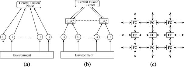
Two well known schemes used by the CFC to incorporate measurements from multiple sensors are sequential updating and parallel updating:
• In the sequential updating scheme, the updating is carried out with the measurement of one sensor at a time. The posterior state estimate obtained from the measurements reported by the kth sensor is used as the prior information when the measurements from the ![]() th sensor is processed. For one specific senor, those techniques commonly used in the single sensor-multitarget tracking problem, like one/two point initialization, multi-frame data association, and Kalman filtering, are applied.
th sensor is processed. For one specific senor, those techniques commonly used in the single sensor-multitarget tracking problem, like one/two point initialization, multi-frame data association, and Kalman filtering, are applied.
• In the parallel updating scheme, the measurements from the various sensors are first associated to yield “supermeasurements,” then these supermeasurements are processed by the CFC as if they were reported by a single sensor. In other words, after the measurement association procedure, the multisensor-multitarget tracking problem has been converted to a single sensor-multitarget tracking problem in the parallel updating scheme.
In the two schemes mentioned above, usually it has been assumed that the sensors are synchronized. In real scenarios, the sensors are seldom perfectly synchronized and too many asynchronous sensors will reduce the optimality of the centralized tracking architecture.
Distributed Tracking: In order to avoid the heavy communication and computational requirement of centralized fusion, distributed or hierarchical architecture, shown in Figure 15.2b, is used alternatively [126]. In this architecture, sensors are connected to Local Fusion Centers (LFCs) and LFCs are in turn connected to a CFC. Each LFC updates its local tracks based on the measurements obtained from the local sensors and sends its tracks state information to CFC. Then, the CFC performs the track-to-track fusion and may send back the updated tracks to the LFCs, if the feedback path is available.
There are two crucial questions in this type of architecture. The CFC needs to decide whether local tracks from different LFCs represent the same target, i.e., the problem of track-to-track association. Furthermore, because of the common process noise or the common prior, the local state estimates for the same target from different LFCs are not independent anymore. Thus, the dependency between the local tracks for the same target from different LFCs has to be handled optimally in the track-track fusion. First, the cross-covariance between the local tracks has to be estimated and then the covariance of the fused track has to be increased correspondingly. Note that, even the above two questions are solved optimally, the distributed tracking architecture is still suboptimal compared to the centralized architecture, because the optimal fusion of the state estimates of local tracks can not provide the same performance as the optimal fusion of the entire data set [9].
To optimally handle the dependency between the local tracks for the same target, the computational cost may be large and the required information may take up too much communication bandwidth, especially when there are many LFCs. Thus, several suboptimal methods are proposed to handle the dependency between the local tracks for the same target. One suboptimal way is using the corresponding tracklets of the local tracks in the CFC for the track-track fusion. A tracklet is a track specially calculated from the local track such that its errors are not cross-correlated with the errors of any other data in the system for the same target [34,35]. Another suboptimal methods is the covariance intersection technique, which takes a convex combination of the estimate of the mean and the information matrix (i.e., the inverse of the covariance matrix) of the local tracks. The covariance intersection method actually provides an estimate of the upper bound of the covariance matrix of the optimally fused track [25,51].
Decentralized tracking: When there is no CFC that can communicate with all LFCs in a large surveillance region, neither centralized nor distributed tracking is possible. In such cases, an alternative called decentralized architecture, shown in Figure 15.2c, is used. Decentralized architecture is composed of multiple Fusion Centers (FCs) and no CFC [126]. Here, each FC gets the measurements from one or more sensors that are connected to it, and uses those measurements to update its tracks. In addition, tracks are also updated whenever an FC gets additional information from its neighbors. Note that even though many FCs are available, each FC can communicate only with its neighbors; the FCs within the communication distance every few measurement time steps. There is no common communication facility in decentralized tracking network, i.e., FC cannot broadcast results and communication must be kept on a strictly neighbor-to-neighbor basis [36]. In decentralized tracking architecture, each FC can be considered as a combination of LFC and CFC, because it updates the track state using measurements from connected sensors and it also does track-track fusion whenever neighboring FCs report their track states. Usually, the algorithms developed for the distributed tracking architecture can be used here without any major modification.
Sensor Registration: The benefits afforded by the integration of data from multiple sensors are greatly diminished if sensor biases are present. In practical systems, sensor states are not precisely specified with respect to some common coordinate system and measurements may be subjected to pointing errors, calibration errors or computational errors. As a result, knowledge about sensor location or attitude may not be accurate. Without this knowledge, there may be severe degradation in the performance of data association, filtering and fusion, leading to eventual loss of track quality. Thus, sensor registration and data alignment is the first step in the fusion process. In sensor registration [5], the bias is estimated and the resulting values are used to debias measurements prior to fusion. Assume that local tracks for the same target from different sensors have already been associated, then to estimate the bias vector, the classical approach is to augment the system state to include the bias vector as part of the state and implement an augmented state Kalman filter (ASKF) [39,54,74]. However, under some circumstances, the prior track-to-track association may be unnecessary for the sensor registration process [64].
3.15.8 Centralized tracking
It is assumed that there are ![]() sensors. The measurement from sensor
sensors. The measurement from sensor ![]() at time
at time ![]() is
is
![]() (15.97)
(15.97)
The measurement noise sequences are zero mean, white, independent of the process noise and independent from sensor to sensor with covariances ![]() . If
. If ![]() , the above problem becomes a single sensor-multitarget tracking problem. Two widely used techniques to incorporate multiple sensors are sequential updating technique and parallel updating technique.
, the above problem becomes a single sensor-multitarget tracking problem. Two widely used techniques to incorporate multiple sensors are sequential updating technique and parallel updating technique.
3.15.8.1 Sequential updating
In sequential updating scheme, the state update is carried out with the measurement of one sensor at a time.
Start the recursion from the predicted state and covariance denoted by
![]() (15.98)
(15.98)
![]() (15.99)
(15.99)
The updates with the measurements at time ![]() are
are
![]() (15.100)
(15.100)
where
![]() (15.101)
(15.101)
![]() (15.102)
(15.102)
The above update scheme shows that, the update step for the jth sensor is almost same as that for the single sensor-multitarget tracking problem. The only difference is that the posterior track state estimates, ![]() , which are obtained after the processing of the
, which are obtained after the processing of the ![]() th sensor’s measurements, is used as the predicted track state
th sensor’s measurements, is used as the predicted track state ![]() for the jth sensor.
for the jth sensor.
For linear measurements, the order of updating in the sequential procedure is immaterial. For nonlinear measurements however, measurement from the most accurate sensor should be updated first so as to reduce subsequent linearization errors.
3.15.8.2 Parallel updating
In parallel updating scheme, measurements generated by the same target from each sensor are associated, and simultaneously stacked and updated. After the measurement-to-measurement association process, the multisensor-multitarget tracking problems has been converted into a single sensor-multitarget tracking problem with the following measurement model:
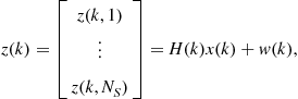 (15.103)
where
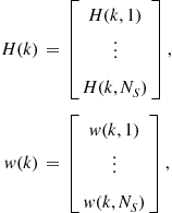
and
![]() (15.104)
(15.104)
The most important step of the parallel updating is the measurement-to-measurement association. If ![]() lists of measurements are obtained from
lists of measurements are obtained from ![]() synchronous sensors, then the goal is to group the measurements that could have originated from the same (unknown) target. In one commonly used approach, each feasible S-tuple of measurement
synchronous sensors, then the goal is to group the measurements that could have originated from the same (unknown) target. In one commonly used approach, each feasible S-tuple of measurement ![]() , consisting one measurement from each sensor, is assigned a cost (typically, a likelihood ratio similar to (15.80)) and then the set of S-tuples that minimizes the global cost is found. This optimization can be formulated as a multidimensional (S-D) assignment as described in Section 3.15.5.0.1.
, consisting one measurement from each sensor, is assigned a cost (typically, a likelihood ratio similar to (15.80)) and then the set of S-tuples that minimizes the global cost is found. This optimization can be formulated as a multidimensional (S-D) assignment as described in Section 3.15.5.0.1.
The unknown target state, which is necessary to find the assignment cost, is replaced by its Maximum Likelihood (ML) estimate:
![]() (15.105)
(15.105)
Note that, if the type of measurements does not have a full observability, then the S-tuple in the association needs to have a certain minimum number of measurements from a target in order for the state of the target to be observable.
3.15.9 Distributed tracking
In a distributed or decentralized configuration, each fusion center has a number of tracks. One crucial question is how to handle the dependency between different local tracks generated by the same target.
There are three sources for the cross correlation between any track pairs for the same target [35]:
1. Common prior information. When the same meaningful prior information is used to initialize new tracks for the same target among different Local Fusion Center (LFC) or the Central Fusion Center (CFC), those tracks will be cross-correlated.
2. Updated tracks including duplicate measurement sequence. Considering a multisensor-multitarget problem with two LFCs and one CFC. For target ![]() , LFC
, LFC ![]() has formed its local track
has formed its local track ![]() only based on its own measurement set
only based on its own measurement set ![]() , respectively. At the end of time
, respectively. At the end of time ![]() , a global track
, a global track ![]() for
for ![]() has been built inside the CFC by fusing
has been built inside the CFC by fusing ![]() . At the end of time
. At the end of time ![]() , the CFC fuses local track
, the CFC fuses local track ![]() and the predicted global track
and the predicted global track ![]() . However,
. However, ![]() , which is predicted from
, which is predicted from ![]() , and
, and ![]() , which is estimated from measurement sequence
, which is estimated from measurement sequence ![]() , both contain the information in measurement sequence
, both contain the information in measurement sequence ![]() , so
, so ![]() and
and ![]() are correlated.
are correlated.
3. Common process noise. If target is maneuvering or the state model used by trackers includes the process noise, then those measurements from the same target will be correlated because they contain the same process noise component.
Thus, if the target is strictly moving with a constant velocity, no process noise is used in LFCs and CFC, each LFC form its tracks strictly based on its own measurement sets (i.e., no feedback from the CFC to the LFC), and the CFC is restarted whenever a new or updated local track was available (i.e., memoryless fusion center), then there will not be any cross-correlation between any track pairs for the same target.
One useful tool to explain and analyze the information dependence due to communication is information graph [26,62]. Information events, such as observation by a sensor at a given time or fusion by a FC at a specific time, are represented by the nodes of the graph. The flow of information is represented by a directed link between the nodes. Thus, a node that is a common predecessor to two nodes contains the common information of those two nodes and the common information of any two or more nodes can be found out by identifying their common predecessors. Information graph is especially useful when the communication structure among FCs is complicated since in this case the identification of common information may not be easy.
3.15.9.1 Cross-covariance of the estimation errors
The dependency between the local state estimation errors for the same target is characterized by the cross-covariances of the local estimation errors, so it is important to estimate the cross-covariance between local track pair [9].
Assume sensors are synchronized, then the recursion for the cross-covariance between local track ![]() and
and ![]() is given by
is given by
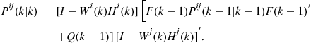 (15.106)
This is a linear recursion and its initial condition is assuming the initial errors to be uncorrelated, i.e., ![]() (no meaningful prior information). This is a reasonable assumption in view of the fact that the initial estimates are usually based on the initial measurements, which are assumed to have independent errors.
(no meaningful prior information). This is a reasonable assumption in view of the fact that the initial estimates are usually based on the initial measurements, which are assumed to have independent errors.
Assume the difference of the estimates of local track ![]() and
and ![]() is
is
![]() (15.107)
(15.107)
then its corresponding covariance is
![]() (15.108)
(15.108)
The above equations indicate that the effect of the dependency between the estimation error is to reduce the covariance of the difference of the estimates of local track ![]() and
and ![]() , because the common process noise and the common prior reduces the positive correlation between the estimation errors. In addition, the dependency between the local tracks from the same target leads to a larger covariance of the fused estimate state than in the case of independent errors. The above calculation of the cross-correlation is optimal only when it has been done synchronously.
, because the common process noise and the common prior reduces the positive correlation between the estimation errors. In addition, the dependency between the local tracks from the same target leads to a larger covariance of the fused estimate state than in the case of independent errors. The above calculation of the cross-correlation is optimal only when it has been done synchronously.
3.15.9.2 Association for tracks with dependent errors
In this algorithm, the problem of associating tracks represented by their local estimates and covariances from ![]() fusion centers is considered [8].
fusion centers is considered [8].
Consider the assignment formulation for track-to-track association from ![]() fusion centers. Assume fusion center
fusion centers. Assume fusion center ![]() has a list of
has a list of ![]() tracks. Define a binary assignment variable
tracks. Define a binary assignment variable ![]() as
as
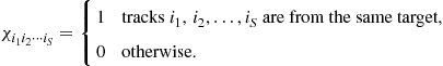 (15.109)
A subset of indices ![]() could be zero in the assignment variable meaning that no track will be from the target in the corresponding list of the fusion centers.
could be zero in the assignment variable meaning that no track will be from the target in the corresponding list of the fusion centers.
The ![]() -D assignment formulation finds the most likely hypothesis by solving the following constrained optimization.
-D assignment formulation finds the most likely hypothesis by solving the following constrained optimization.
 (15.110)
subject to the constraints
 (15.111)
 (15.112)
![]() (15.113)
(15.113)
 (15.114)
and
![]() (15.115)
(15.115)
In (15.110) the assignment cost is
![]() (15.116)
(15.116)
where ![]() is the likelihood ratio of the track association hypothesis vs. all tracks from extraneous targets. The following equation can be used to calculate
is the likelihood ratio of the track association hypothesis vs. all tracks from extraneous targets. The following equation can be used to calculate ![]()
 (15.117)
where ![]() is the diffuse pdf of track density,
is the diffuse pdf of track density, ![]() is the number of elements in
is the number of elements in ![]() and
and
![]() (15.118)
(15.118)
and ![]() is its covariance matrix. From (15.108), the diagonal blocks in
is its covariance matrix. From (15.108), the diagonal blocks in ![]() are
are
![]() (15.119)
(15.119)
and off-diagonal blocks are
![]() (15.120)
(15.120)
The Maximum Likelihood (ML) estimate of the track states obtained by fusing the set of tracks ![]() is given by
is given by
![]() (15.121)
(15.121)
where ![]() is
is ![]() matrix and
matrix and ![]() is the dimension of the state vector. Also,
is the dimension of the state vector. Also,
![]() (15.122)
(15.122)
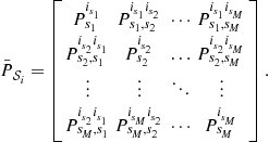 (15.123)
The covariance matrix of the fused track is given by
![]() (15.124)
(15.124)
3.15.9.3 Tracklet fusion
A tracklet is a track computed so that its state estimation error is not cross-correlated with the state estimation errors of any other data in the system for the same target. There are two types of methods to build tracklet [35]:
1. Form a tracklet by decorrelating a local track.
2. Form a tracklet directly from a sequence of measurements.
Both of them ignore the cross correlation caused by the common process noise. Furthermore, as being pointed out in [35], only the tracklet-from-track type of methods can be used to decorrelate the cross correlation from the common prior information. Thus, in this chapter, only the tracklet-from-track type of methods are discussed. In the following, ![]() and
and ![]() represent the predicted track state and covariance matrix in the
represent the predicted track state and covariance matrix in the ![]() th LFC.
th LFC. ![]() and
and ![]() represent the posterior track state and covariance matrix in the
represent the posterior track state and covariance matrix in the ![]() th LFC.
th LFC. ![]() is the state transfer matrix from the
is the state transfer matrix from the ![]() th scan to the
th scan to the ![]() th scan.
th scan.
There are three methods falling in tracklet-from-track category [35]:
1. Inverse Kalman filter (Frenkel’s Method No. 1). It outputs ![]() for a local track
for a local track ![]() from LFC
from LFC ![]() at time
at time ![]() , given that the local track was previously reported by the same LFC to the CFC at frame
, given that the local track was previously reported by the same LFC to the CFC at frame ![]() . Tracklet
. Tracklet ![]() and its covariance are calculated by:
and its covariance are calculated by:
![]() (15.125)
(15.125)
![]() (15.126)
(15.126)
![]() (15.127)
(15.127)
![]() (15.128)
(15.128)
![]() (15.129)
(15.129)
The input to the CFC is ![]() , the equivalent measurement, and
, the equivalent measurement, and ![]() , its corresponding measurement error covariance matrix. The equivalent measurement equation matrix
, its corresponding measurement error covariance matrix. The equivalent measurement equation matrix ![]() for
for ![]() in the CFC is an identity matrix. The global track estimate
in the CFC is an identity matrix. The global track estimate ![]() has to be predicted to frame
has to be predicted to frame ![]() . This method cannot be used if there is only one measurement in the tracklet interval
. This method cannot be used if there is only one measurement in the tracklet interval ![]() .
.
2. Tracklet with decorrelated state estimate (Frenkel’s Method No. 2). It outputs ![]() for a local track
for a local track ![]() from LFC
from LFC ![]() at time
at time ![]() , given that the track data was previously reported by the same LFC to the CFC at frame
, given that the track data was previously reported by the same LFC to the CFC at frame ![]() . Tracklet
. Tracklet ![]() and its covariance are calculated by:
and its covariance are calculated by:
![]() (15.130)
(15.130)
![]() (15.131)
(15.131)
![]() (15.132)
(15.132)
![]() (15.133)
(15.133)
![]() (15.134)
(15.134)
![]() (15.135)
(15.135)
The input to the CFC is ![]() and its corresponding covariance matrix
and its corresponding covariance matrix ![]() . The equivalent measurement equation matrix
. The equivalent measurement equation matrix ![]() for
for ![]() in the CFC is
in the CFC is ![]() . Still, the estimate of global track
. Still, the estimate of global track ![]() has to be predicted to
has to be predicted to ![]() . This method can be used even when there is only one measurement in the tracklet interval
. This method can be used even when there is only one measurement in the tracklet interval ![]() .
.
3. Inverse information filter [9,36,104]. It outputs ![]() for a local track
for a local track ![]() from local tracker
from local tracker ![]() at time
at time ![]() , given that the track data was previously sent by the same LFC to the CFC at frame
, given that the track data was previously sent by the same LFC to the CFC at frame ![]() . Tracklet
. Tracklet ![]() and its covariance are calculated by:
and its covariance are calculated by:
![]() (15.136)
(15.136)
![]() (15.137)
(15.137)
![]() (15.138)
(15.138)
![]() (15.139)
(15.139)
The input to the CFC is ![]() and its corresponding covariance matrix
and its corresponding covariance matrix ![]() . Note, to use
. Note, to use ![]() and
and ![]() directly, the CFC should run the information filter (i.e., inverse Kalman filter).
directly, the CFC should run the information filter (i.e., inverse Kalman filter).
Since the received tracklets are assumed to be independent of each other and independent of the local tracks, tracklets association problem can be solved by using an ![]() -D association technique, where the set of tracklets are treated as the set of measurements with independent measurement noise.
-D association technique, where the set of tracklets are treated as the set of measurements with independent measurement noise.
3.15.9.4 Covariance intersection
When cross-correlation between two estimations is unknown and hard to calculate, a sub-optimal information fusion algorithm, called Covariance Intersection (CI) algorithm, is proposed in [51]. It takes a convex combination of the estimation of the mean and the information matrix (the inverse of the covariance matrix) and can provide a consistent fused estimate. Here the consistency for the estimate ![]() of unknown state
of unknown state ![]() is defined as:
is defined as:
![]() (15.140)
(15.140)
Assume there are two independent sensors, ![]() and
and ![]() , to observe one target. Each sensor is equipped with a Kalman filter and based on its measurement sequence, at time
, to observe one target. Each sensor is equipped with a Kalman filter and based on its measurement sequence, at time ![]() , two consistent estimate of target state
, two consistent estimate of target state ![]() are obtained from sensor
are obtained from sensor ![]() and sensor
and sensor ![]() , respectively. Now the information from
, respectively. Now the information from ![]() , has to be fused to get
, has to be fused to get ![]() , a better estimation of target state. Furthermore,
, a better estimation of target state. Furthermore, ![]() has to be consistent.
has to be consistent.
In the CI algorithm, a linear convex combination formula is used to fuse ![]() and
and ![]() :
:
![]() (15.141)
(15.141)
![]() (15.142)
(15.142)
where ![]() is determined by minimizing the trace or the determinant of
is determined by minimizing the trace or the determinant of ![]() . In both cases, the cost function is convex respect to
. In both cases, the cost function is convex respect to ![]() and the semidefinite convex programming technique can be used to solve this minimization problem. To avoid the time consuming optimization procedure in the CI algorithm, two fast algorithms to calculate the weight
and the semidefinite convex programming technique can be used to solve this minimization problem. To avoid the time consuming optimization procedure in the CI algorithm, two fast algorithms to calculate the weight ![]() has been proposed in [37,89].
has been proposed in [37,89].
The intuition behind the CI algorithm comes from the geometric interpretation of covariance matrixes ![]() and
and ![]() . Just as shown in Fig. 1 of [51], no matter what the cross-correlation between
. Just as shown in Fig. 1 of [51], no matter what the cross-correlation between ![]() and
and ![]() is, the theoretical optimal
is, the theoretical optimal ![]() always lies within the intersection of two ellipsoids that represent
always lies within the intersection of two ellipsoids that represent ![]() respectively. Thus, if the fused covariance matrix,
respectively. Thus, if the fused covariance matrix, ![]() , encloses the intersection region, it must be consistent even if there is no knowledge about the cross-correlation
, encloses the intersection region, it must be consistent even if there is no knowledge about the cross-correlation ![]() . Actually, the fused covariance from (15.142) can be thought as a Gaussian approximation of the actual covariance intersection. Obviously, the tighter the updated covariance encloses the intersection region, the greater the amount of information which can be used. The consistent of the fused covariance has guaranteed that the estimation is non-divergent.
. Actually, the fused covariance from (15.142) can be thought as a Gaussian approximation of the actual covariance intersection. Obviously, the tighter the updated covariance encloses the intersection region, the greater the amount of information which can be used. The consistent of the fused covariance has guaranteed that the estimation is non-divergent.
From the intuition behind the CI algorithm, it is clear that a significant drawback of the CI algorithm in [51] is that it will inevitably over estimate the fused covariance matrix and will lead to unnecessary loss in its calculated fusion accuracy. As pointed out in [25], if all local trackers give the same covariance matrix estimations, i.e., ![]() , then there is
, then there is ![]() no matter how many estimates have been fused. In other words, under this circumstance, the error bound provided by
no matter how many estimates have been fused. In other words, under this circumstance, the error bound provided by ![]() does not represent any possible reduction in the uncertainty of the fused estimate. This phenomenon has been explained in [25] using the set estimation theory. Based on the unknown but bounded set estimation theory, a tighter bound for the fused covariance matrix is given in [25]. There, given two local tracker’s estimation
does not represent any possible reduction in the uncertainty of the fused estimate. This phenomenon has been explained in [25] using the set estimation theory. Based on the unknown but bounded set estimation theory, a tighter bound for the fused covariance matrix is given in [25]. There, given two local tracker’s estimation ![]() , it assumes that the unknown target state
, it assumes that the unknown target state ![]() lies inside two ellipsoids
lies inside two ellipsoids ![]() , respectively, and the ellipsoid is defined as
, respectively, and the ellipsoid is defined as
![]() (15.143)
(15.143)
Given ![]() can only be in their intersection area, which may not be ellipsoid. However, a bounding ellipsoid for this intersection, which satisfy
can only be in their intersection area, which may not be ellipsoid. However, a bounding ellipsoid for this intersection, which satisfy ![]() , can be defined as
, can be defined as
![]() (15.144)
(15.144)
where ![]() . With some algebra simplification, the above formula comes into:
. With some algebra simplification, the above formula comes into:
![]() (15.145)
(15.145)
in which ![]() follows (15.141), (15.142), respectively and
follows (15.141), (15.142), respectively and ![]() is given by:
is given by:
![]() (15.146)
(15.146)
Thus, the fused covariance matrix has been shrink from ![]() to
to ![]() .
.
3.15.10 Performance evaluation
In this section, the Posterior Cramér-Rao Lower Bound (PCRLB) of tracking [10,44,46,47,115], which provides a minimum bound of any tracking estimation, and several tracker-related metrics, which measure the performance of multitarget trackers in cardinality, time and accuracy [40,66,103], are discussed.
3.15.10.1 Posterior Cramér-Rao Lower Bound (PCRLB)
3.15.10.1.1 Background
Let ![]() be an unknown and random state vector, and let
be an unknown and random state vector, and let ![]() be an unbiased estimate of
be an unbiased estimate of ![]() based on the measurement data,
based on the measurement data, ![]() . The PCRLB, which is defined to be the inverse of the Fisher Information Matrix (FIM),
. The PCRLB, which is defined to be the inverse of the Fisher Information Matrix (FIM), ![]() [117], then gives a lower bound of the error covariance matrix, i.e.,
[117], then gives a lower bound of the error covariance matrix, i.e.,
![]() (15.147)
(15.147)
where ![]() denotes expectation over (
denotes expectation over (![]() ,
, ![]() ) and
) and ![]() denotes the transpose. The inequality in (15.147) means that
denotes the transpose. The inequality in (15.147) means that ![]() is a positive semi-definite matrix.
is a positive semi-definite matrix.
A recursive formula for the evaluation of the posterior FIM, ![]() , is given by [116]:
, is given by [116]:
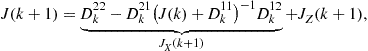 (15.148)
![]() (15.149)
(15.149)
![]() (15.150)
(15.150)
![]() (15.151)
(15.151)
![]() (15.152)
(15.152)
![]() (15.153)
(15.153)
and ![]() is a second-order partial derivative operator whose
is a second-order partial derivative operator whose ![]() th term is given by
th term is given by
![]() (15.154)
(15.154)
![]() and
and ![]() are the ith components of vectors
are the ith components of vectors ![]() and
and ![]() , respectively. In the above,
, respectively. In the above, ![]() , where
, where ![]() is the measurement vector at sensor
is the measurement vector at sensor ![]() at sampling time
at sampling time ![]() and
and ![]() is the number of sensors utilized at sampling time
is the number of sensors utilized at sampling time ![]() .
.
3.15.10.1.2 Dynamic system contribution to the PCRLB
Let the state vector at time ![]() , obtained by stacking the state vectors of all targets, be denoted by
, obtained by stacking the state vectors of all targets, be denoted by ![]() , where
, where ![]() is the state vector of target
is the state vector of target ![]() and
and ![]() is the total number of targets in the surveillance region. If we assume that targets are moving independently and the state equation of each target is linear, then the overall state equation is given by
is the total number of targets in the surveillance region. If we assume that targets are moving independently and the state equation of each target is linear, then the overall state equation is given by
![]() (15.155)
(15.155)
where
![]() (15.156)
(15.156)
![]() (15.157)
(15.157)
In the above, ![]() is the state transition matrix and
is the state transition matrix and ![]() is the process noise of target
is the process noise of target ![]() . If
. If ![]() is Gaussian with zero mean and covariance
is Gaussian with zero mean and covariance ![]() , then the covariance matrix of
, then the covariance matrix of ![]() ,
, ![]() , is given by
, is given by
![]() (15.158)
(15.158)
It can be shown that in the case of linear, Gaussian dynamics (e.g., [101]) we have
![]() (15.159)
(15.159)
![]() (15.160)
(15.160)
![]() (15.161)
(15.161)
Using the Matrix Inversion Lemma and (15.159)–(15.161) , there is
![]() (15.162)
(15.162)
The matrix ![]() gives the prior information regarding the target states at time
gives the prior information regarding the target states at time ![]() .
.
Besides process noise, sometimes the dynamic model uncertainty also contributes to the PCRLB, especially in the case of maneuvering targets, whose kinematics model may evolve in a time-varying manner. Thus, it is necessary to consider the PCRLB for a filtering problem with multiple switching dynamic models and additive Gaussian noise. Some related works can be found in [48,109].
3.15.10.1.3 Measurement contribution to the PCRLB
The measurement contribution to the PCRLB is given by ![]() . Consider the general case in which there is measurement origin uncertainty, with measurements originating from one of the targets or from clutter. The jth measurement at the ith sensor is given by
. Consider the general case in which there is measurement origin uncertainty, with measurements originating from one of the targets or from clutter. The jth measurement at the ith sensor is given by
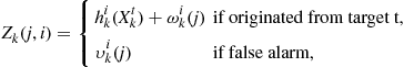 (15.163)
where ![]() is (in general) a nonlinear function,
is (in general) a nonlinear function, ![]() is a zero mean Gaussian random variable with covariance
is a zero mean Gaussian random variable with covariance ![]() and
and ![]() is uniformly distributed across the surveillance region
is uniformly distributed across the surveillance region ![]() (with hyper-volume,
(with hyper-volume, ![]() ). The probability mass function of the number of false alarms,
). The probability mass function of the number of false alarms, ![]() , which is Poisson-distributed with mean
, which is Poisson-distributed with mean ![]() , is given by
, is given by
![]() (15.164)
(15.164)
where ![]() is the number of false alarms and
is the number of false alarms and ![]() is the spatial density of the false alarms.
is the spatial density of the false alarms.
When multiple targets are present, the association between the measurements and the targets is not known and must be considered in the PCRLB calculation. The following assumptions are made regarding the measurements:
• Each measurement can be generated by one of the targets or the clutter.
• Each target can produce zero or one measurement at any one time.
If sensors have independent measurement processes, ![]() can be written as [114]
can be written as [114]
![]() (15.165)
(15.165)
where
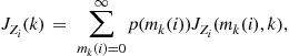 (15.166)
![]() (15.167)
(15.167)
In the above equations, ![]() is the number of sensors used at time
is the number of sensors used at time ![]() and
and ![]() is the number of measurements at sensor
is the number of measurements at sensor ![]() at time
at time ![]() .
.
The probability of receiving ![]() measurements,
measurements, ![]() , from sensor
, from sensor ![]() is given by
is given by
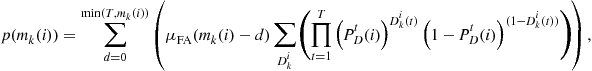 (15.168)
where ![]() is the detection vector that indicates which targets are detected at sensor
is the detection vector that indicates which targets are detected at sensor ![]() (at time
(at time ![]() ).1 The total number of targets that are detected is
).1 The total number of targets that are detected is ![]() , i.e.,
, i.e., ![]() .
. ![]() is the probability of detection of target
is the probability of detection of target ![]() by sensor
by sensor ![]() .
.
The probability density function of the measurement ![]() conditioned on
conditioned on ![]() and
and ![]() is given by [49]
is given by [49]
![]() (15.169)
(15.169)
where ![]() is the association vector that indicates which measurement originated from which target. Each element
is the association vector that indicates which measurement originated from which target. Each element ![]() of
of ![]() is a random variable that takes a value in
is a random variable that takes a value in ![]() , with 0 indicating a false alarm.
, with 0 indicating a false alarm. ![]() indicates that the measurement
indicates that the measurement ![]() originates from target
originates from target ![]() . If the targets are well separated in the measurement space, there is no measurement origin uncertainty in terms of targets and any one measurement can be originated from a known target or clutter [114]. However, if the targets are closely-spaced or cross one another, it is hard to find the association vector and all possible associations must be considered in the calculation of measurement information
. If the targets are well separated in the measurement space, there is no measurement origin uncertainty in terms of targets and any one measurement can be originated from a known target or clutter [114]. However, if the targets are closely-spaced or cross one another, it is hard to find the association vector and all possible associations must be considered in the calculation of measurement information ![]() .
.
It has been shown in [115] that ![]() th block of
th block of ![]() is given as follows:
is given as follows:
![]() (15.170)
(15.170)
where
![]() (15.171)
(15.171)
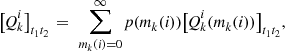 (15.172)
and ![]() denotes the
denotes the ![]() th element of matrix
th element of matrix ![]() .
. ![]() is the Information Reduction Matrix (IRM) for sensor
is the Information Reduction Matrix (IRM) for sensor ![]() and
and ![]() is the
is the ![]() th block of the IRM.
th block of the IRM. ![]() is also given in [115]. No closed form analytical solution exists for the IRM
is also given in [115]. No closed form analytical solution exists for the IRM ![]() , which must then be calculated using a numerical integration technique.
, which must then be calculated using a numerical integration technique.
3.15.10.2 Tracker-related measures for performance evaluation
Generally, a tracker-related measure is defined as a function getting ![]() , and
, and ![]() as inputs and providing some measures that evaluate the quality of the tracking algorithm. Here,
as inputs and providing some measures that evaluate the quality of the tracking algorithm. Here, ![]() is defined as the collection of all tracks,
is defined as the collection of all tracks, ![]() is the total information of truth, and
is the total information of truth, and ![]() is the set of all measurements. The following categories are considered for the tracker-related measures [40]:
is the set of all measurements. The following categories are considered for the tracker-related measures [40]:
• Tracker-dependent:
These measures are developed for individual types of trackers. For example, performance measures have been specially defined for IMM filters [65,124], for assignment based tracking algorithms [46], for dynamic programming [50], MHT trackers [20] and IPDA algorithm [125]. This group of metrics is also called algorithm based metrics because they are defined for a specific type of tracking and filtering method, or a specific application, and may not be applicable to other tracking methods.
• Tracker-independent:
These types of measures can be applied to every tracker. Various categories can be again defined based on the availability of truths and tracks. When truths and tracks are both available, a large class of performance metrics can be defined after finding an association between the estimated tracks and available truths. In real scenarios, sometimes truths are not available. In this case, statistical tests are done on the estimated tracking results to check the consistency of the estimates. The type of metrics is also called algorithm free metrics.
In this subsection, only the tracker-independent metrics are reviewed, because only these type of the tracker-related measures can be applied to every tracking algorithms. Different categories of algorithm free metrics may be defined based on the availability of truths and tracking results as
• Available truths and tracks:
This is the most popular and applicable case in performance evaluation when the goal is to evaluate tracking results with the known truths. There are three classes of metrics summarized as follows:
• Track Cardinality Measures:
This metric measures numerical characteristics of obtained results. For example, the number of confirmed tracks associated with truths, and number of missed and false tracks can be considered as cardinality measures. The major limitation of these measures is that they do not provide any information about the performance of individual tracks, such as the consistency of track and the accuracy of estimation. Also, no information is available about the time characteristics of the estimated tracks.
• Time (Durational) Measures:
Time performance of estimated tracks is evaluated by this class of metrics. These performance measures provide information about the persistency of a track. For example, track probability of detection is represented as a metric evaluating the detection ability of a tracker in estimating every truth. Unlike cardinality measures, time metrics can provide more useful information about the duration or persistency of estimated tracks.
• Accuracy Measures:
This is the most common measure evaluating the closeness of estimated values to the truths. Several measures can be defined based on the type of distance between the set of truths and tracks. For example, the root mean squared error (RMSE) of target estimation is the most common criterion used in the literature in which a traditional Mahanabolis distance is derived to compute the error. Some other measures might be also defined based on other types of distances. To evaluate the quality of the tracking algorithm in track cardinality and state accuracy jointly, the Optimal Subpattern Assignment (OSPA) metric has been proposed in [107]. The OSPA metric in [107] is the summation of two terms, one term measures the cardinality error when the number of tracks is not equal to the number of truth while the other term gives the localization error. However, the track’s label is not considered in [107], so the OSPA metric in [107] is unable to measure the track labeling error or the track identity swap. To take into consideration that each track normally has a label and identity, an extension of the OSPA metric has been proposed in [102]. Furthermore, by replacing the criterion from minimizing the RMSE to minimizing the mean OSPA, a new type of multitarget filters, the set-JPDA filter and the set-MHT algorithm, have been proposed in [30,110].
• Available tracks and unknown truths:
This case is very common in real scenarios when there is no information about truths. In this situation, the consistency of tracking results may be checked. The innovation of tracking is used as the main source of information and, then, common statistical tests may be made on the received information. There are also other scoring metrics defined in [21].
Above performance evaluation is mainly discussed for a single sensor case. For a multiple sensor problem, performance measures may be found separately for each sensor and, afterwards, a final metric is extracted by fusing individual measures. This method is used for the distributed tracking methods when sensors estimate the state of targets independently. For the centralized case [4], the multiple sensor can be treated as a single sensor case with a group of unique estimates for targets of interest. The measure of performance is then found for the estimated states [4].
3.15.11 Simulations—a multiple closely-spaced target scenario
In this subsection, several tracker-related measures of performance are applied to a simulated scenario in order to demonstrate the application of several multitarget tracking algorithms [40]. The following tracking algorithms are applied in this subsection:
• Interactive Multiple Model-Hypothesis-Oriented Multiple Hypothesis Tracker (IMM-HOMHT) [12].
• Interactive Multiple Model-Track Oriented Multiple Hypothesis Tracker (IMM-TOMHT) [12].
• Multiple Model-Gaussian Mixture Probability Hypothesis Density Filter (IMM-GM-PHD) [93].
• Multiple Model-Cardinalized Gaussian Mixture Probability Hypothesis Density Filter (IMM-GM-CPHD).
• Interactive Multiple Model-SD Assignment (IMM-SD) [97].
• Interactive Multiple Model-Joint Integrated Probability Data Association (IMM-JIPDA) [119].
• Interactive Multiple Model-2D Assignment (IMM-SD-2D) [97].
Parameters of every tracker are adjusted according to the scenario used for the simulation. An EKF algorithm is used in the filtering stage of all algorithms. Three different types of motion models are used for the IMM filter: the Constant Velocity (CV) model, the Constant Acceleration (CA) model and the Constant Turn (CT) [10] model. Although it is possible that every tracker uses its own selection of motion models, in order to provide a good comparison here the same models are used as IMM modes in every trackers. In order to deal with time varying number of targets, ![]() logic and track quality methods are used to initialize new-born targets and delete dead ones [4]. The values of
logic and track quality methods are used to initialize new-born targets and delete dead ones [4]. The values of ![]() and
and ![]() depend on the scenario and tracking algorithm. Except JIPDA algorithm and PHD filters that utilize quality-based method for track management, other methods use
depend on the scenario and tracking algorithm. Except JIPDA algorithm and PHD filters that utilize quality-based method for track management, other methods use ![]() logic. Once the estimated tracks are obtained, the tracking results as well as the truths are both used to calculate performance metrics. For the PHD and the CPHD filter, unique tag is attached to each Gaussian component and a JIPDA type algorithm is used for the track management. For the TOMHT, an enumeration based algorithm is used to approximately search the best global hypothesis. Table 15.1 summarizes the general parameters that are common among all scenarios.
logic. Once the estimated tracks are obtained, the tracking results as well as the truths are both used to calculate performance metrics. For the PHD and the CPHD filter, unique tag is attached to each Gaussian component and a JIPDA type algorithm is used for the track management. For the TOMHT, an enumeration based algorithm is used to approximately search the best global hypothesis. Table 15.1 summarizes the general parameters that are common among all scenarios.
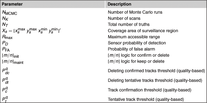
A challenging multiple target scenario is used in this section in order to evaluate the performance of trackers in dealing with closely-spaced targets [55].
Parameters of the simulated scenario are described as follows:
• Sensors and scenario parameters:
A single sensor is used to generate the measurements of targets. Measurements are gathered in terms of range and bearing [10]. The variance of the range and bearing measurements are chosen to be ![]() and
and ![]() , respectively. Parameters of the underlying scenario are presented in Table 15.2.
, respectively. Parameters of the underlying scenario are presented in Table 15.2.

• Target parameters:
Figure 15.3 shows the generated trajectories of targets in the surveillance region. It can be observed that although all targets are well-separated initially, most of them approach each other in the subsequent scans. In other words, there are several crossing targets in this scenario that makes the tracking problem challenging. Due to the non-maneuvering movement of targets, a CV model is used to characterize the motion of every target.
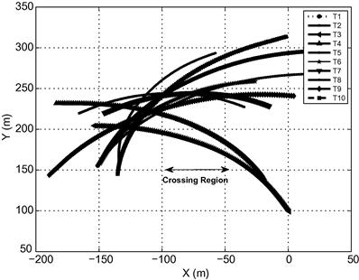
• Trackers:
Table 15.3 presents common parameters for all trackers. Note that PHD algorithm uses quality-based method for track management where ![]() are chosen to be
are chosen to be ![]() . Also, IMM-JIPDA tracker utilizes a quality-based approach for track management with
. Also, IMM-JIPDA tracker utilizes a quality-based approach for track management with ![]() ,
, ![]() , and
, and ![]() as the parameters.
as the parameters.
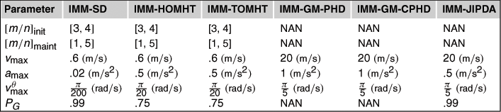
The tracking results as well as available truths are used to calculate performance metrics. Figure 15.4 shows the performance evaluator, which is designed by the ETF Lab, ECE Department, McMaster University, and this performance evaluator is used in the chapter to calculate and present metrics. Metrics have been classified into time, cardinality and accuracy measures.

For graphical interpretations, the results of three metrics are shown in Figures 15.5–15.7. For the precise definition of each metric, please refer to [40]. Also, the average results are presented in Tables 15.4–15.6 for the analysis over every individual tracker. In all tables, T1 to T6 stand for IMM-SD, IMM-JIPDA, IMM-HOMHT, IMM-TOMHT, IMM-GM-PHD, IMM-GM-CPHD, respectively. It can be seen that all trackers achieve, relatively the same detection performance in terms of track probability of detection. From Figure 15.6, it can be concluded that all targets have been well detected by trackers because measure of completeness shows a value very close to one for all trackers. Note that, there is no dense clutter area in this scenario. Therefore, the average number of false tracks shows a small value for all trackers. Nevertheless, the main difficulty of this scenario is the presence of crossing and closely-spaced targets that may affect the continuity measure and number of breaks and swaps. As the Table 15.4 shows, MHT trackers provide the lowest measure of continuity. It can be seen that IMM-HOMHT generates the most number of breaks in tracks leading to the lowest continuity measure. IMM-JIPDA tracker provides results with acceptable number of breaks even though there are many swaps in the estimated tracks that results in representing IMM-JIPDA as the third-worst tracker in terms of the continuity measure. These results show that, when using the parameters listed in Table 15.3, MHT and JIPDA trackers cannot provide satisfactory results compared to SD and PHD trackers, becuase the probability of breaks and swaps gets higher due to the presence of closely-spaced targets. Also, the tables show the superiority of IMM-SD tracker in terms of the majority of metrics over other trackers.
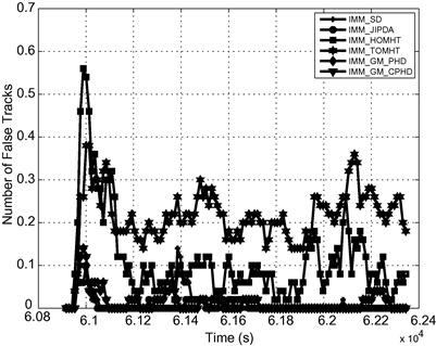
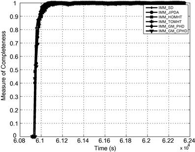

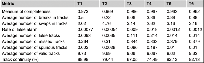
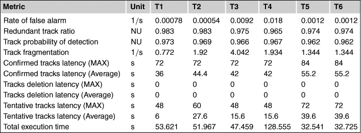
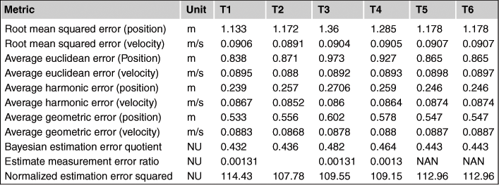
As a conclusion, it can be observed that, with parameters listed in Table 15.3, IMM-SD tracker has been able to provide the most accurate results with the least number of breaks and swaps in the tested tracks. MHT and JIPDA cannot track available targets continually although the detection capability of trackers are still comparable with other trackers. PHD filters stand between the best tracker and MHT and JIPDA trackers with satisfactory detection and continuity measures. It should be noted that theoretically the IMM-SD tracker can be considered as an implementation of IMM-TOMHT and both two trackers should provide the same performance. However, the simulation results show that the IMM-SD tracker works better than the IMM-TOMHT. One explanation is that the global optimal hypothesis is obtained thorough the enumeration in the current IMM-TOMHT tracker, so there is no guarantee that the hypothesis found by the current IMM-TOMHT is the real optimal one. On the other hand, in IMM-SD tracker, Lagrange Relaxation method is used to get an approximated optimal global hypothesis.
3.15.12 Summary
In this chapter, various filters, data-association techniques, multitarget tracking algorithms, multisensor-multitarget architectures and measures of performance were discussed in detail for the multisensor-multitarget tracking problem. Various combinations of these algorithms provide a complete tracking and fusion framework for multisensor networks with application to civilian as well as military problems. For example, the tracking and fusion techniques discussed here are applicable to fields like air traffic control, air/ground/maritime surveillance, mobile communication, transportation, video monitoring and biomedical imaging/signal processing. Using a scenario with many closely-spaced targets, it was also shown that the algorithms discussed here are all capable of handling the challenging multitarget tracking problem.
Relevant Theory: Signal Processing Theory and Machine Learning
See Vol. 1, Chapter 4 Random Signals and Stochastic Processes
See Vol. 1, Chapter 11 Parametric Estimation
See Vol. 1, Chapter 12 Adaptive Filters
See Vol. 1, Chapter 19 A Tutorial Introduction to Monte Carlo Methods, Markov Chain Monte Carlo and Particle Filtering
References
1. Ackerson GA, Fu KS. On state estimation in switching environments. IEEE Trans Automat Control. 1970;15(1):10–17.
2. Alouani AT, Gray JE, McCabe DH. Theory of distributed estimation using multiple asynchronous sensors. IEEE Trans Aerosp Electron Syst. 2005;41(2):717–722.
3. Arulampalam MS, Maskell S, Gordon N, Clapp T. A tutorial on particle filters for online nonlinear/non-Gaussian Bayesian tracking. IEEE Trans Signal Process. 2002;50(2):174–188.
4. Bar-Shalom Y, Blair WD. Multitarget/Multisensor Tracking: Applications and Advances. Artech House October 2000.
5. Bar-Shalom Y. Airborne GMTI radar position bias estimation using static-rotator targets of opportunity. IEEE Trans Aerosp Electron Syst. 2001;37(2):695–699.
6. Bar-Shalom Y. Dimensionless score function for multiple hypothesis tracking. IEEE Trans Aerosp Electron Syst. 2007;43(1):392–400.
7. Bar-Shalom Y, Challa S, Blom HAP. IMM estimator versus optimal estimator for hybrid systems. IEEE Trans Aerosp Electron Syst. 2005;41(3):986–991.
8. Bar-Shalom Y, Chen H. Multisensor track-to-track association for tracks with dependent errors. J Adv Inform Fusion. 2006;1(1):3–14.
9. Bar-Shalom Y, Willett P, Tian X. Tracking and Data Fusion: A Handbook of Algorithm. Storrs, CT: YBS Publishing; 2011.
10. Bar-Shalom Y, Li XR, Kirubarajan T. Estimation with Applications to Tracking and Navigation. Wiley 2001.
11. Bar-Shalom Y, Kirubarajan T, Gokberk C. Tracking with classification-aided multiframe data association. IEEE Trans Aerosp Electron Syst. 2005;41(3):868–878.
12. Blackman SS. Multiple hypothesis tracking for multiple target tracking. IEEE Aerosp Electron Syst Mag. 2004;19(1, Part 2):5–18.
13. Blackman SS, Popoli R. Design and Analysis of Modern Tracking Systems. Artech House 1999.
14. Blair WD, Watson GA, Kirubarajan T, Bar-Shalom Y. Benchmark for radar resource allocation and tracking in the presence of ECM. IEEE Trans Aerosp Electron Syst. 1998;34(4):1097–1114.
15. Blom HAP. A sophisticated tracking algorithm for ATC surveillance data. In: Proceedings of the International Radar Conference, Paris. May 1984;393–398.
16. Blom HAP, Bar-Shalom Y. The interacting multiple model algorithm for systems with Markovian switching coefficients. IEEE Trans Automat Control. 1988;33(8):780–783.
17. Capponi A, De Waard HW. A mean track approach applied to the multidimensional assignment problem. IEEE Trans Aerosp Electron Syst. 2007;43(2):450–471.
18. Chang CB, Athans M. State estimation for discrete system with switching parameters. IEEE Trans Aerosp Electron Syst. 1978;14(3):418–425.
19. Chen H, Kirubarajan T, Bar-Shalom Y. Performance limits of track-to-track fusion versus centralized estimation: theory and application. IEEE Trans Aerosp Electron Syst. 2003;39(2):386–400.
20. Chang KC, Mori S, Chong CY. Evaluating a multiple-hypothesis multitarget tracking algorithm. IEEE Trans Aerosp Electron Syst. 1994;30(2):578–590.
21. Chang KC, Zhao X. A greedy assignment algorithm and its performance evaluation. In: Proceedings of American Control Conference, Seattle, USA. June 1995.
22. Chang KC, Saha RK, Bar-Shalom Y. On optimal track-to-track fusion. IEEE Trans Aerosp Electron Syst. 1997;33(4):1271–1276.
23. Chen X, Tharmarasa R, Pelletier M, Kirubarajan T. Integrated clutter estimation and target tracking using Poisson point processes. IEEE Trans Aerosp Electron Syst. 2012;48(2):1210–1235.
24. Chong CY. Distributed architectures for data fusion. In: Proceedings of the First International Conference on Information Fusion, Las Vegas, NV. August 1998.
25. Chong CY, Mori S. Convex combination and covariance intersection algorithms in distributed fusion. In: Proceedings of the Fourth International Conference on Information Fusion, Montreal, QC, Canada. August 2001.
26. Chong CY, Mori S. Distributed fusion and communication management for target identification. In: Proceedings of the Eighth International Conference on Information Fusion, Philadelphia, PA. July 2005.
27. Chummun MR, Kirubarajan T, Pattipati KR, Bar-Shalom Y. Fast data association using multidimensional assignment with clustering. IEEE Trans Aerosp Electron Syst. 2001;37(3):898–913.
28. Coman CI, Kreitmair T. Evaluation of the tracking process in ground surveillance applications. In: Proceedings of the Sixth European Radar Conference, Rome, Italy. September 2009.
29. Coraluppi S, Grimmett D, de Theije P. Benchmark evaluation of multistatic trackers. In: Proceedings of the Sixth International Conference on Information Fusion, Florance, Italy. July 2006.
30. Crouse DF, Willett P, Svensson L, Svensson D, Guerriero M. The set MHT. In: Proceedings of the 14th International Conference on Information Fusion, Chicago, IL. July 2011.
31. Daum F. Nonlinear filters: beyond the Kalman filter. IEEE Aerosp Electron Syst Mag. 2005;20(8, Part 2):57–69.
32. Deb S, Yeddanapudi M, Pattipati KR, Bar-Shalom Y. A generalized S-dimensional assignment for multisensor-multitarget state estimation. IEEE Trans Aerosp Electron Syst. 1997;33(2):523–538.
33. Doucet A, de Freitas N, Gordon N. Sequential Monte Carlo Methods in Practice. New York: Springer-Verlag; 2001.
34. Drummond OE. A hybrid sensor fusion algorithm architecture and tracklets. In: July 1997;485–502. Proceedings of SPIE Conference on Signal and Data Processing of Small Targets, San Diego, CA. vol. 3163.
35. Drummond OE. Track and tracklet fusion filtering using data from distributed sensors. In: Proceedings of Estimation, Tracking and Fusion: A Tribute to Yaakov Bar-Shalom, Monterey, CA. May 2001;167–186.
36. Durrant-Whyte H, Stevens M. Data fusion in decentralised sensing networks. In: Proceedings of the Fourth International Conference on Information Fusion, Montreal, QC, Canada. August 2001.
37. Fränken D, Hüpper A. Improved fast covariance intersection for distributed data fusion. In: Proceedings of the Seventh International Conference on Information Fusion, Stockholm, Sweden. July 2005.
38. Gordon NJ, Salmond DJ, Smith AFM. Novel approach to nonlinear/non-Gaussian Bayesian state estimation. IEE Proc Radar Signal Process. 1993;140(2):107–113.
39. Gordon NJ, Ristic B, Robinson M. Performance bounds for recursive sensor registration. In: Proceedings of the Sixth International Conference on Information Fusion, Cairns, Australia. July 2003.
40. Gorji AA, Tharmarasa R, Kirubarajan T. Performance measures for multiple target tracking problems. In: Proceedings of 14th International Conference on Information Fusion, Chicago, US. July 2011.
41. Grimmett D, Coraluppi S, La Cour BR, et al. MSTWG multistatic tracker evaluation using simulated scenario data sets. In: Proceedings of the 11th International Conference on Information Fusion, Cologne, Germany. September 2008.
42. Harishan K, Tharmarasa R, Kirubarajan T, Thayaparan T. Automatic track initialization and maintenance in heavy clutter using integrated JPDA and ML-PDA algorithms. In: September 2011; Proceedings of SPIE Conference on Signal and Data Processing of Small Targets, San Diego, CA. vol. 8137.
43. Hanselmann T, Mus̆icki D, Palaniswami M. Adaptive target tracking in slowly changing clutter. In: Proceedings of the Ninth International Conference on Information Fusion, Florence, Italy. July 2006.
44. Hernandez ML, Marrs AD, Gordon NJ, Maskell SR, Reed CM. Cramér-Rao bounds for non-linear filtering with measurement origin uncertainty. In: Proceedings of the Fifth International Conference on Information Fusion, Annapolis, USA. 2002.
45. Hernandez ML, Kirubarajan T, Bar-Shalom Y. Multisensor resource deployment using posterior Cramér-Rao bounds. IEEE Trans Aerosp Electron Syst. 2004;40(2):399–416.
46. Hernandez ML, Ristic B, Farina A, Timmoneri L. A comparison of two Cramér-Rao lower bounds for nonlinear filtering with ![]() . IEEE Trans Signal Process. 2004;52(9):2361–2370.
. IEEE Trans Signal Process. 2004;52(9):2361–2370.
47. Hernandez ML, Farina A, Ristic B. A PCRLB for tracking in cluttered environments: measurement sequence conditioning approach. IEEE Trans Aerosp Electron Syst. 2006;42(2):680–704.
48. Hernandez ML, Ristic B, Farina A, Sathyan T, Kirubarajan T. Performance measure for Markovian switching systems using best-fitting Gaussian distributions. IEEE Trans Aerosp Electron Syst. 2008;44(2):724–747.
49. Hue C, Le Cadre JP, Pérez P. Performance analysis of two sequential Monte Carlo methods and posterior Cramér-Rao bounds for multitarget tracking. In: July 2002;464–473. Proceedings of the Fifth International Conference on Information Fusion, Annapolis, MD. vol. 1.
50. Johnston LA, Krishnamurthy V. Performance evaluation of a dynamic programming track before detect algorithm. IEEE Trans Aerosp Electron Syst. 2002;38(1):228–242.
51. Julier SS, Uhlmann JK. A non-divergent estimation algorithm in the presence of unknown correlations. In: Proceedings of American Control Conference, Albuquerque, New Mexico. June 1997.
52. Julier SJ, Uhlmann JK. A new extension of the Kalman filter to nonlinear systems. In: April 1997;182–193. Proceedings of SPIE Conference on Signal Processing, Sensor Fusion and Target Recognition VI, Orlando, FL. vol. 3068.
53. Kalman RE. A new approach to linear filtering and prediction problems. Trans ASME—J Basic Eng. 1960;82:34–45.
54. Kastella K, Yeary B, Zadra T, Brouillard R, Frangione E. Bias modeling and estimation for GMTI applications. In: Proceedings of the Third International Conference on Information Fusion, Paris, France. July 2000.
55. Kirubarajan T, Bar-Shalom Y, McAllister R, Schutz R, Engelberg B. Multitarget tracking using an IMM estimator with debiased E-2C measurements for AEW systems. In: Proceedings of the Second International Conference on Information Fusion, Sunnyvale, CA. July 1999.
56. Kirubarajan T, Bar-Shalom Y. Kalman filter versus IMM estimator: when do we need the latter? IEEE Trans Aerosp Electron Syst. 2003;39(4):1452–1457.
57. Kirubarajan T, Bar-Shalom Y. Probabilistic data association techniques for target tracking in clutter. Proc IEEE. 2004;92(3):536–557.
58. Kirubarajan T, Bar-Shalom Y, Lerro D. Bearings-only tracking of maneuvering targets using a batch-recursive estimator. IEEE Trans Aerosp Electron Syst. 2001;37(3):770–780.
59. Kirubarajan T, Wang H, Bar-Shalom Y, Pattipati KR. Efficient multisensor fusion using multidimensional data association. IEEE Trans Aerosp Electron Syst. 2001;37(2):386–400.
60. Kreucher C, Kastella K, Hero III AO. Multitarget tracking using the joint multitarget probability density. IEEE Trans Aerosp Electron Syst. 2005;41(4):1396–1414.
61. Lefebvre T, Bruyninckx H, De Schutter J. Kalman filters for non-linear systems: a comparison of performance. Int J Control. 2004;77:639–653.
62. Liggins ME, Chong CY, Kadar I, Alford MG, Vannicola V, Thomopoulos S. Distributed fusion architectures and algorithms for target tracking. Proc IEEE. 1997;85(1):95–107.
63. Lin L, Bar-Shalom Y, Kirubarajan T. New assignment-based data association for tracking move-stop-move targets. IEEE Trans Aerosp Electron Syst. 2004;40(2):714–725.
64. Lin X, Kirubarajan T, Bar-Shalom Y. Multisensor bias estimation with local tracks without a priori association. In: August 2003; Proceedings of SPIE Conference on Signal and Data Processing of Small Targets, San Diego, CA. vol. 5204.
65. Li XR, Bar-shalom Y. Performance prediction of interacting multiple model algorithm. IEEE Trans Aerosp Electron Syst. 1993;29.
66. Li XR, Zhao Z. Evaluation of estimation algorithms Part I: Incomprehensive measures of performance. IEEE Trans Aerosp Electron Syst. 2006;42(5):1340–1358.
67. Li XR, Li N. Integrated real-time estimation of clutter density for tracking. IEEE Trans Signal Process. 2000;48(10):2797–2805.
68. Li N, Li XR. Target perceivability and its applications. IEEE Trans Signal Process. 2001;49(11):2588–2604.
69. Li XR, Jilkov V. Survey of maneuvering target tracking Part III Measurement models. In: July 2001; Proceedings of SPIE Conference on Signal and Data Processing of Small Targets, San Diego, CA. vol. 4473.
70. Li XR, Jilkov V. Survey of maneuvering target tracking Part IV Decision-based methods. In: April 2002; Proceedings of SPIE Conference on Signal and Data Processing of Small Targets, Orlando, FL. vol. 4728.
71. Li XR, Jilkov V. Survey of maneuvering target tracking Part I Dynamic models. IEEE Trans Aerosp Electron Syst. 2003;39(4):1333–1364.
72. Li XR, Jilkov V. Survey of maneuvering target tracking Part V Multiple-model methods. IEEE Trans Aerosp Electron Syst. 2005;41(4):1255–1321.
73. Li XR, Jilkov V. Survey of maneuvering target tracking Part II Motion models of ballistic and space targets. IEEE Trans Aerosp Electron Syst. 2010;46(1):96–119.
74. Lin X, Bar-Shalom Y, Kirubarajan T. Multisensor multitarget bias estimation for general asynchronous sensors. IEEE Trans Aerosp Electron Syst. 2005;41(3):899–921.
75. R. Mahler, An Introduction to Multisensor-Multitarget Statistics and its Application, Lockheed Martin Technical Monograph, 2000.
76. Mahler R. Multi-target moments and their application to multi-target tracking. In: Proceedings of the Workshop on Estimation, Tracking and Fusion: A Tribute to Yaakov Bar-Shalom, Monterey, CA. 2001;134–166.
77. Mahler R. Random set theory for target tracking and identification. In: Hall DL, Lindas J, eds. Handbook of Multisensor Data Fusion. Boca Raton, FL: CRC Press; 2002; (Chapter 14).
78. Mahler R. Multitarget bayes filtering via first-order multitarget moments. IEEE Trans Aerosp Electron Syst. 2003;39(4):1152–1178.
79. Mahler R. PHD filter of higher order in target number. IEEE Trans Aerosp Electron Syst. 2007;43(4):1523–1541.
80. Mahler R. The multisensor PHD filter: I General solution via multitarget calculus. In: April 2009; Proceedings of SPIE Conference on Signal Processing, Sensor Fusion and Target Recognition XVIII, Orlando, FL. vol. 7336.
81. Mahler R. CPHD and PHD filters for unknown backgrounds I: Dynamic data clustering. In: 2009; Proceedings of SPIE Conference on Sensors and Systems for Space Applications III, Orlando, FL, USA. vol. 7330.
82. Mahler R. CPHD and PHD filters for unknown backgrounds II: Multitarget filtering in dynamic clutter. In: 2009; Proceedings of SPIE Conference on Sensors and Systems for Space Applications III, Orlando, FL, USA. vol. 7330.
83. Mahler R. Approximate multisensor CPHD and PHD filters. In: Proceedings of 10th International Conference on Information Fusion, Edinburgh, UK. July 2010.
84. Mallick M, Scala BL. Comparison of single-point and two-point difference track initiation algorithms using position measurements. Acta Automat Sinica. 2008;34(3):258–265.
85. Mušicki D, Evans R, Stankovic S. Integrated probabilistic data association. IEEE Trans Automat Control. 1994;39(6):1237–1241.
86. Mušicki D, Evans R. Joint integrated probabilistic data association: JIPDA. IEEE Trans Aerosp Electron Syst. 2004;40(3):1093–1099.
87. Mušicki D, Suvorova S, Morelande M, Mora B. Clutter map and target tracking. In: Proceedings of Eighth International Conference on Information Fusion, Wyndham Philadelphia, PA, USA. July 2005;69–76.
88. Mušicki D, Evans R. Multiscan multitarget tracking in clutter with integrated track splitting filter. IEEE Trans Aerosp Electron Syst. 2009;45(4):1432–1447.
89. Niehsen W. Information fusion based on fast covariance intersection filtering. In: Proceedings of the Fifth International Conference on Information Fusion, Annapolis, Washington DC Area. July 2002.
90. Okello N, Ristic B. Maximum likelihood registration for multiple dissimilar sensors. IEEE Trans Aerosp Electron Syst. 2003;39(3):1074–1083.
91. Panta K, Clarak DE, Vo BN. Data association and track management for the Gaussian mixture probability hypothesis density filter. IEEE Trans Aerosp Electron Syst. 2009;45(3):1003–1016.
92. Pulford GW. Taxonomy of multiple target tracking methods. Proc IEE Radar Sonar Navig. 2005;152(5):291–304.
93. Pasha SA, Vo BN, Ma WK. A Gaussian mixture PHD filter for jump Markov system models. IEEE Trans Aerosp Electron Syst. 2009;45(3):919–936.
94. Pattipati KR, Deb S, Bar-Shalom Y, Washburn RB. A new relaxation algorithm and passive sensor data association. IEEE Trans Automat Control. 1992;37(2):198–213.
95. Pattipati KR, Kirubarajan T, Popp RL. Survey of assignment techniques for multitarget tracking. In: Proceedings of the Workshop on Estimation, Tracking, and Fusion: A Tribute to Yaakov Bar-Shalom, Monterey, CA. May 2001.
96. Popp RL, Pattipati KR, Bar-Shalom Y. Dynamically adaptable m-best 2D assignment and multi-level parallelization. IEEE Trans Aerosp Electron Syst. 1999;35(4):1145–1160.
97. Popp RL, Kirubarajan T, Pattipati KR. Survey of assignment techniques for multitarget tracking. In: Bar-Shalom Y, Blair WD, eds. Multitarget/Multisensor Tracking: Applications and Advances III. Artech House 2000; (Chapter 2).
98. Punithakumar K, Kirubarajan T, Sinha A. Multiple-model probability hypothesis density filter for tracking maneuvering targets. IEEE Trans Aerosp Electron Syst. 2008;44(1):87–98.
99. Panta K, Ba-Ngu V, Singh S. Novel data association schemes for the probability hypothesis density filter. IEEE Trans Aerosp Electron Syst. 2007;43(2):556–570.
100. Ristic B, Arulampalam S, Gordon N. Beyond the Kalman Filter: Particle Filters for Tracking Applications. Artech House Publishers 2004.
101. Ristic B, Zollo S, Arulampalam S. Performance bounds for maneuvering target tracking using asynchronous multi-platform angle-only measurements. In: Proceedings of the Fourth International Conference on Information Fusion, Montreal, Quebec. August 2001.
102. Ristic B, Vo B-N, Clark D, Vo B-T. A metric for performance evaluation of multi-target tracking algorithms. IEEE Trans Signal Process. 2011;59(7):3452–3457.
103. Rothrock R, Drummond OE. Performance metrics for multiple-sensor, multiple-target tracking. In: Proceedings of SPIE Conference on Signal and Data Processing of Small Targets, Orlando, USA. July 2000.
104. Ridley M, Nettleton E, Sukkarieh S, Durrant-Whyte H. Tracking in decentralised air-ground sensing. In: Proceedings of the Fifth International Conference on Information Fusion, Annapolis, MD. August 2002.
105. Sarkka S. On unscented Kalman filtering for state estimation of continuous-time nonlinear systems. IEEE Trans Automat Control. 2007;52(9):1631–1641.
106. Sathyan T, Sinha A, Kirubarajan T. Computationally efficient assignment-based algorithms for data association for tracking with angle-only sensors. In: August 2007; Proceedings of SPIE Conference on Signal and Data Processing of Small Targets, San Diego, CA. vol. 6699.
107. Schuhmacher D, Vo B-T, Vo B-N. A consistent metric for performance evaluation of multi-object filters. IEEE Trans Signal Process. 2008;56(8):3447–3457.
108. Schuhmacher D, Vo B-T, Vo B-N. On performance evaluation of multi-object filters. In: Proceedings of the 13th International Conference on Information Fusion, Edinburgh, Scotland. July 2010.
109. Svensson L. On Bayesian Cramér-Rao bound for Markovian switching systems. IEEE Trans Signal Process. 2010;58(9):4507–4516.
110. Svensson L, Svensson D, Guerriero M, Willett P. Set JPDA filter for multitarget tracking. IEEE Trans Signal Process. 2011;59(10):4677–4691.
111. Shea PJ, Zadra T, Klamer D, Frangione E, Brouilard R, Kastella K. Precision tracking of ground targets. In: Proceedings of IEEE Aerospace Conference, Big Sky, MT. March 2000.
112. Sidenbladh H. Multi-target particle filtering for the probability hypothesis density. In: July 2003;800–806. Proceedings of the Sixth International Conference on Information Fusion. vol. 2.
113. Smith D, Singh S. Approaches to multisensor data fusion in target tracking: a survey. IEEE Trans Knowledge Data Eng. 2006;18(12):1696–1710.
114. Tharmarasa R, Kirubarajan T, Hernandez ML. Large-scale optimal sensor array management for multitarget tracking. IEEE Trans Syst Man Cybernet. 2007;37(5):803–814.
115. Tharmarasa R, Kirubarajan T, Hernandez ML, Sinha A. PCRLB-based multisensor array management for multitarget tracking. IEEE Trans Aerosp Electron Syst. 2007;43(2):539–555.
116. Tichavsky P, Muravchik CH, Nehorai A. Posterior Cramér-Rao bounds for discrete-time nonlinear filtering. IEEE Trans Signal Process. 1998;46(5):1386–1396.
117. Van Trees H. Detection, Estimation and Modulation Theory. vol. I New York: Wiley; 1968.
118. van Doorn BA, Blom HAP. Systematic error estimation, in multisensor fusion systems. In: Proceedings of SPIE Conference on Signal and Data Processing of Small Targets, Orlando, FL. April 1993.
119. Vermaak J, Godsill SJ, Perez P. Monte Carlo filtering for multi-target tracking and data association. IEEE Trans Aerosp Electron Syst. 2005;41(1):309–322.
120. Vo B-N, Singh S, Doucet A. Sequential Monte Carlo implementation of the PHD filter for multi-target tracking. In: July 2003;792–799. Proceedings of the Sixth International Conference on Information Fusion. vol. 2.
121. Vo B-N, Ma WK. The Gaussian mixture probability hypothesis density filter. IEEE Trans Aerosp Electron Syst. 2006;54(11):4091–4104.
122. Vo B-T, Vo B-N, Cantoni A. Analytic implementations of the cardinalized probability hypothesis density filter. IEEE Trans Aerosp Electron Syst. 2007;55(7):3553–3567.
123. Wan EA, van der Merwe R. The unscented Kalman filter, for nonlinear estimation. In: Proceedings of IEEE, Adaptive Systems for Signal Processing, Communications, and Control Symposium, Alberta, Canada. October 2000.
124. Wang H, Kirubarajan T, Bar-Shalom Y. Precision large scale air traffic surveillance using an IMM estimator with assignment. IEEE Trans Aerosp Electron Syst. 1999;35(1):255–266.
125. Wang X, Musicki D. Evaluation of IPDA type filters with a low elevation sea-surface target tracking. In: Proceedings of the Sixth International Conference on Information Fusion, Queensland, Australia. May 2003.
126. Xiong N, Svensson P. Multi-sensor management for information fusion: issues and approaches. Inform Fusion. 2002;3(1):163–186.
127. You H, Jingwei Z. New track correlation algorithms in a multisensor data fusion system. IEEE Trans Aerosp Electron Syst. 2006;42(4):1359–1371.
128. Zhan R, Wan J. Iterated unscented Kalman filter for passive target tracking. IEEE Trans Aerosp Electron Syst. 2007;43(3):1155–1163.
1![]() takes the value 1 if target
takes the value 1 if target ![]() is detected and 0 otherwise.
is detected and 0 otherwise.