
MIMO Radar with Widely Separated Antennas—From Concepts to Designs
Qian He*, Yang Yang† and Rick S. Blum†, *Department of Electronic Engineering, University of Electronic Science and Technology of China, Chengdu, Sichuan, China, †Department of Electrical and Computer Engineering, Lehigh University, Bethlehem, PA, USA, [email protected], [email protected], [email protected]
Abstract
This chapter focuses on multiple-input and multiple-output (MIMO) radar with widely dispersed antennas. The concept of and difference between coherent and noncoherent configurations are introduced. Both parameter estimation and target detection using MIMO radar are considered, and the corresponding accuracy and complexity problems are investigated. Approaches for achieving phase synchronization among different radar sensors are provided. Optimum waveform design methods are discussed. Theoretical analysis and numerical simulations demonstrate the good performance of the MIMO radar with widely separated antennas using the presented methods.
Keywords
Detection; Estimation; Multiple-input multiple-output (MIMO) radar; Phase synchronization; Waveform design
2.13.1 Introduction
Recent advances in wireless communications featuring the innovative multiple-input multiple-output (MIMO) technology [1] have catalyzed a wave of interest in understanding and exploiting the concept of MIMO radar, e.g., [2–7]. The similarity between MIMO communications and MIMO radar systems that employ widely separated antennas is rather intriguing: in communications, MIMO systems combat the fading effects of the multipath channel through its spatial diversity advantage; in radar, the complex targets consisting of several scatterers resemble very much the multipath channel in wireless communications, and likewise, MIMO radar with widely separated antennas also offers the diversity gain. To be more specific, a target’s radar cross section (RCS), which determines the amount of returned power, varies greatly with respect to the considered aspect angle. Those variations can significantly degrade the ability of a conventional radar in detecting and estimating the target. MIMO radar with widely separated antennas, whereas, through observing a target simultaneously from different (uncorrelated) aspect angles, provide spatial diversity which can substantially countervail the fluctuations in received power.
Since the inception of MIMO radar in the early 2000s, a great deal of efforts have been devoted to studying its performance potentials or developing a variety of application paradigms for it, e.g., [8–13]. However, note that MIMO radar systems studied in most of the literature can be roughly classified into two categories. The first category features the use of closely spaced antennas [3], i.e., the array configuration of these radars is close to that of the conventional phased array radar. But the utilization of specific (e.g., orthogonal) transmit waveforms in this type of MIMO radar systems can render many benefits which are, otherwise, not achievable with the conventional phased array radars. The second category, as surveyed in [4], takes advantage of multiple transmit signals as well. But it employs widely separated antennas at both the transmit and receive ends, and thus enjoys the spatial diversity gain.
Among all these widely-separated-antenna cases are two cases that have received special attention: one called coherent MIMO radar and the other called noncoherent MIMO radar [4]. The distinguishing features are whether the target reflection model is coherent and whether the processing is coherent. For the case of coherent MIMO radar, the antennas are within a given target beamwidth1 which leads to identical (coherent) reflection coefficients, and a coherent processing approach is adopted. While for the case of noncoherent MIMO radar, the antennas lie in different target beamwidths which leads to distinct (noncoherent) reflection coefficients, and a noncoherent processing approach is adopted. The coherent processing requires phase synchronization of the oscillators employed at widely separated antennas, while the noncoherent processing does not. In fact, phase synchronization embodies a major difference between the operations of noncoherent MIMO radar and coherent MIMO radar, as will be mathematically demonstrated later in this chapter.
In this document, we will focus on the MIMO radar with widely separated antennas. Although far from being exhaustive, this document strives to summarize and discuss a large range of issues related to this particular type of MIMO radar—both coherent and noncoherent processing approaches included. Topics of interest encompass those with strong theoretical significance, for example, performance evaluation of both coherent and noncoherent MIMO radar in target localization and velocity estimation, study of diversity gain for MIMO radar under the Neyman-Pearson (NP) criteria, etc. Topics of realistic values are also covered, which include, for example, phase synchronization algorithm design for coherent MIMO radar, and MIMO radar waveform design for extended targets. Through reviewing some state of the art in this area, ranging from theoretical concepts to practical designs, this document is intended to serve as an easy beginning as well as a handy reference for researchers who have interest in delving into this field. It is also expected to foster further discussions on those related research topics, and to spur further research interest within this field.
The remainder of this document is organized as follows. In Section 2.13.2, after a brief introduction to the coherent MIMO radar, we derive the mean square error (MSE) of the maximum likelihood (ML) estimate and the Cramer-Rao bound (CRB) for joint target location and velocity estimation, and investigate the impact of static phase errors at the transmitters and receivers on the performance of target localization. In Section 2.13.3, we turn our attention to noncoherent MIMO radar. Parallel to the study for the coherent case, the joint estimation for target location and velocity using noncoherent MIMO radar is presented, the MSE of the ML estimate is analyzed, and the CRB is calculated. Then, the noncoherent MIMO radar ambiguity function (AF) is introduced. In Section 2.13.4, we discuss the MSE performance differences between coherent and noncoherent MIMO radars in the application of joint target location and velocity estimation. We demonstrate that the magnitude of these differences decreases with an increase in the product of the number of transmit and receive antennas, when the antennas for both coherent and noncoherent systems are properly placed. In Section 2.13.5, we derive the diversity gain for a MIMO radar system adopting the Neyman-Pearson detection. The relationship between the cumulative distribution function (cdf) of the reflection coefficients, the cdf of the clutter-plus-noise, and the signal space dimension of the transmitted waveforms is described. In Section 2.13.6, we present three phase synchronization approaches for coherent MIMO radar, which include the master-slave closed-loop method, the round-trip approach, and the broadcast consensus based algorithm. We compare these three phase synchronization approaches and discuss some issues that may arise in practice. In Section 2.13.7, we introduce some waveform design schemes for MIMO radar with widely separated antennas. Finally we conclude this document with a summary in Section 2.13.8.
2.13.2 Coherent MIMO radar
Before exposing readers to a variety of interesting issues related to the coherent MIMO radar, we firstly introduce some settings that hold true for both the coherent and noncoherent MIMO radars, which lays a common ground for the subsequent analysis. Let us consider a MIMO radar which is equipped with ![]() transmitters and
transmitters and ![]() receivers. The positions of the
receivers. The positions of the ![]() th,
th, ![]() transmitter and the
transmitter and the ![]() th,
th, ![]() receiver are
receiver are ![]() and
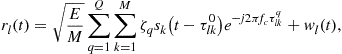
and ![]() respectively, in a two-dimensional Cartesian coordinate system. The lowpass equivalent of the signal transmitted from the
respectively, in a two-dimensional Cartesian coordinate system. The lowpass equivalent of the signal transmitted from the ![]() th transmitter is
th transmitter is ![]() , where
, where ![]() denotes the total transmitted energy, and the waveform is normalized such that
denotes the total transmitted energy, and the waveform is normalized such that
![]() (13.1)
(13.1)
Assume a target, if present, is located at ![]() and moving with velocity
and moving with velocity ![]() . The time delay
. The time delay ![]() and Doppler shift
and Doppler shift ![]() involved in the path from transmitter
involved in the path from transmitter ![]() to receiver
to receiver ![]() , via the target reflection, are
, via the target reflection, are
 (13.2)
and
![]() (13.3)
(13.3)
where ![]() is the speed of light,
is the speed of light, ![]() denotes the distance between the target and the
denotes the distance between the target and the ![]() th transmitter,
th transmitter, ![]() denotes the distance between the target and the
denotes the distance between the target and the ![]() th receiver, and
th receiver, and ![]() represents the wavelength of the carrier with frequency
represents the wavelength of the carrier with frequency ![]() . In both the coherent and noncoherent MIMO radars we assume all transmitter and receiver nodes have oscillators which are locked in frequency, possibly due to the use of a beacon. For the coherent MIMO radar, we also assume these oscillators are locked in phase.
. In both the coherent and noncoherent MIMO radars we assume all transmitter and receiver nodes have oscillators which are locked in frequency, possibly due to the use of a beacon. For the coherent MIMO radar, we also assume these oscillators are locked in phase.
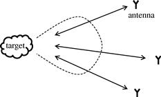
Throughout this chapter, we use the term coherent MIMO radar to refer to MIMO radar system employing coherent processing of received signals obeying a coherent target reflection model. If we model the target as an antenna then we can define an equivalent target beamwidth based on the target size [2]. In a coherent MIMO radar system, the antennas are assumed to be all within the same target beamwidth, as illustrated in Figure 13.1. In this case, the effective target reflection coefficient is assumed to be identical for each transmitter-target-receiver path (which gives a coherent target reflection model) and is denoted by ![]() . We assume
. We assume ![]() is unknown but deterministic. Thus, the received signal at receiver
is unknown but deterministic. Thus, the received signal at receiver ![]() can be modeled as
can be modeled as
 (13.4)
![]() (13.5)
(13.5)
where ![]() represents the clutter-plus-noise component at the
represents the clutter-plus-noise component at the ![]() th receiver for any given time
th receiver for any given time ![]() , and
, and
![]() (13.6)
(13.6)
![]()
represents the signal transmitted from transmitter ![]() and received by receiver
and received by receiver ![]() . Collecting the time delayed and Doppler shifted signals from all paths in an
. Collecting the time delayed and Doppler shifted signals from all paths in an ![]() block diagonal matrix, we arrive at
block diagonal matrix, we arrive at
 (13.7)
Then, the signals received at all ![]() antennas can be written as
antennas can be written as
![]() (13.8)
(13.8)
where
![]() (13.9)
(13.9)
represents the clutter-plus-noise vector, which is assumed to be a zero mean Gaussian random vector that satisfies
![]() (13.10)
(13.10)
with ![]() assumed to be a known2 time invariant constant matrix that determines the clutter-plus-noise covariance matrix at the output of the matched filters.
assumed to be a known2 time invariant constant matrix that determines the clutter-plus-noise covariance matrix at the output of the matched filters.
2.13.2.1 Joint location and velocity estimation
Let the signals observed by a MIMO radar system be
![]() (13.11)
(13.11)
which is a realization of the random vector ![]() in (13.8), we hope to jointly estimate the target location and velocity in the maximum likelihood (ML) sense. As discussed in [15], the ML estimates of the unknown parameters can be found by examining the corresponding log-likelihood ratio. Stack the parameters of interest into a vector as follows:
in (13.8), we hope to jointly estimate the target location and velocity in the maximum likelihood (ML) sense. As discussed in [15], the ML estimates of the unknown parameters can be found by examining the corresponding log-likelihood ratio. Stack the parameters of interest into a vector as follows:
![]() (13.12)
(13.12)
and define a bigger vector
![]() (13.13)
(13.13)
to include all the unknown parameters involved. Using the signal model in (13.8), it can be derived that the log-likelihood ratio with respect to ![]() is given by [16]
is given by [16]
 (13.14)
where ![]() is a constant independent of the parameters to be estimated,
is a constant independent of the parameters to be estimated,
![]() (13.15)
(13.15)
and3
![]() (13.16)
(13.16)
The vector ![]() can be regarded as the output of a matched filter which considers the correlations allowed in the given analysis. It can be shown that, for any value of
can be regarded as the output of a matched filter which considers the correlations allowed in the given analysis. It can be shown that, for any value of ![]() , the ML estimate of
, the ML estimate of ![]() (i.e.,
(i.e., ![]() and
and ![]() ) is [16]
) is [16]
 (13.17)
Then, substituting ![]() in (13.14), it yields
in (13.14), it yields
![]() (13.18)
(13.18)
Note that in (13.18) we changed the notation in the parenthesis to emphasize that, after we have the ML estimate for ![]() , the parameters which need to be estimated are the elements of
, the parameters which need to be estimated are the elements of ![]() . Thus, the ML estimate of the unknown parameter vector
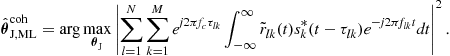
. Thus, the ML estimate of the unknown parameter vector ![]() can be expressed as
can be expressed as
![]() (13.19)
(13.19)
It is worth noting that the estimator (13.19) combines signals from different antennas in a coherent way, but we skip the discussion for now and postpone the explanation after (13.22) until some simplifying assumptions are introduced.
In the previous discussions, the clutter-plus-noise was assumed to be temporally white but possibly spatially colored. In order to simplify the analysis, in the following, we introduce two additional assumptions: orthogonal transmitted signals and spatially white clutter-plus-noise. Leveraging these assumptions, we are able to simplify the problem to be tackled and provide a handful of analytical results, which can not only characterize some typical behaviors of the system when these assumptions are satisfied, but can as well render insight into the system behaviors for cases where these assumptions do not hold. Since these analytical results are relatively easy to obtain and explain, we are also able to shed light on the relationship between the system performance and a few important system parameters. Due to the convenience afforded by these assumptions, we will use them repeatedly in the rest of this chapter.
Assumption 1
Assume the transmitted signals are approximately orthogonal
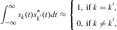
and maintain approximate orthogonality for time delays ![]() ,
,![]() and Doppler shifts
and Doppler shifts![]() of interest so that
of interest so that
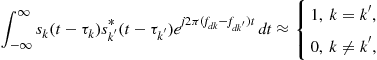
such that the signals contributed from different transmitters can be separated at each receiver. See Appendix A.1 for further discussion.
Assumption 2
The clutter-plus-noise corresponding to the![]() th path
th path![]() is a temporally white zero-mean complex Gaussian random process with
is a temporally white zero-mean complex Gaussian random process with![]() , where
, where![]() is a constant and
is a constant and![]() is a unit impulse function. The clutter-plus-noise components are spatially white, such that
is a unit impulse function. The clutter-plus-noise components are spatially white, such that![]() if
if![]() or
or![]() .
.
Under Assumption 1, it can be obtained that ![]()
![]() . Assumption 2 leads to
. Assumption 2 leads to ![]() , which can be regarded as a result of perfect whitening if the covariance matrix of
, which can be regarded as a result of perfect whitening if the covariance matrix of ![]() , called
, called ![]() previously, can be accurately estimated. Then, we have
previously, can be accurately estimated. Then, we have ![]() and
and ![]() .
.
Applying these results into (13.14), we get a simplified log-likelihood ratio
 (13.20)
where ![]() represents the observed signal corresponding to the received signal model for the
represents the observed signal corresponding to the received signal model for the ![]() th path
th path
![]() (13.21)
(13.21)
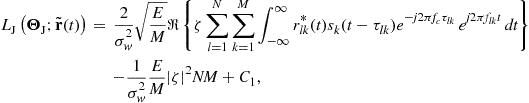
Likewise, applying the simplification assumption to (13.19) gives the simplified ML estimate
 (13.22)
In the estimator in (13.22), phase shifts imposed on various paths have a measurable impact on the estimation output via the term ![]() . Intuitively, we want the terms inside the
. Intuitively, we want the terms inside the ![]() to add together in phase to maximize (13.22), so as to achieve high estimation performance. This is the motivation for the coherent processing (see Appendix A.2 for a distinction between coherent and noncoherent processing). To make the best use of the phase information, phase synchronization is required, so that all transmitters and receivers employ a common phase reference. Some approaches for achieving phase synchronization are described in Section 2.13.6. Note that under Assumptions 1 and 2, the coherent processing is optimal for the coherent target reflection model in Figure 13.1.
to add together in phase to maximize (13.22), so as to achieve high estimation performance. This is the motivation for the coherent processing (see Appendix A.2 for a distinction between coherent and noncoherent processing). To make the best use of the phase information, phase synchronization is required, so that all transmitters and receivers employ a common phase reference. Some approaches for achieving phase synchronization are described in Section 2.13.6. Note that under Assumptions 1 and 2, the coherent processing is optimal for the coherent target reflection model in Figure 13.1.
The mean square error (MSE), the average squared difference between an estimate and the true value of the parameter being estimated, is a useful metric for forecasting the performance of an estimator. The MSE of any unbiased estimator is lower bounded by the Cramer-Rao bound (CRB). Since attaining the MSE is often computationally expensive, the CRB that indicates the best MSE an estimator can provide, serves as an important tool for evaluating the estimation performance and system configuration. In (13.22), we have derived the ML estimator for the coherent MIMO radar joint location and velocity estimation problem. It is known that the ML estimator is asymptotically unbiased, and the MSE of the ML estimate asymptotically approaches the CRB. Thus, we can derive the CRBs for the parameters of interest to provide an approximate MSE of the corresponding ML estimates in the asymptotic region. The Fisher information matrix (FIM) with respect to ![]() can be derived from the log-likelihood function in (13.20) as follows [15,17]
can be derived from the log-likelihood function in (13.20) as follows [15,17]

Under Assumptions 1 and 2, according to the derivations provided in Appendix A.3, we obtain the FIM as shown below:
 (13.23)
where


with the terms ![]() ,
, ![]() ,
, ![]() determined by the target position and velocity, and the antenna positions. The terms
determined by the target position and velocity, and the antenna positions. The terms ![]() ,
, ![]() , and
, and ![]() in
in ![]() are dependent on the characteristics of the received waveforms
are dependent on the characteristics of the received waveforms
![]() (13.24)
(13.24)
![]() (13.25)
(13.25)
![]() (13.26)
(13.26)
![]() (13.27)
(13.27)
and
![]() (13.28)
(13.28)
where ![]() represents the Fourier transform of
represents the Fourier transform of ![]() . The CRBs for the estimates of the unknown target locations and velocities are the first four diagonal elements of the inverse of the FIM
. The CRBs for the estimates of the unknown target locations and velocities are the first four diagonal elements of the inverse of the FIM
![]()
![]() (13.29)
(13.29)
The CRBs can be used to optimize system configurations with respect to certain parameters. Collect the parameters of interest (![]() ) in a vector as
) in a vector as ![]() . These parameters could be, for example, the number of antennas, the antenna placement, the waveform parameters, and so forth. Suppose we require the optimum system configuration design to minimize a metric formed by the weighted sum of the CRBs of the estimates of
. These parameters could be, for example, the number of antennas, the antenna placement, the waveform parameters, and so forth. Suppose we require the optimum system configuration design to minimize a metric formed by the weighted sum of the CRBs of the estimates of ![]() , and
, and ![]() . Then, the value of
. Then, the value of ![]() that optimizes this metric can be expressed as
that optimizes this metric can be expressed as
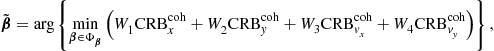 (13.30)
where ![]() are weighting factors and
are weighting factors and ![]() represents the feasible set of
represents the feasible set of ![]() . Numerical methods may be needed to solve this problem. A concrete example of finding the optimum antenna placement for the MIMO radar velocity estimation is provided in [18], where only
. Numerical methods may be needed to solve this problem. A concrete example of finding the optimum antenna placement for the MIMO radar velocity estimation is provided in [18], where only ![]() and
and ![]() are involved and equal weighting is considered, and it is shown analytically that under certain conditions only symmetrical placement can be optimum. Interested readers are referred to [18] for more details.
are involved and equal weighting is considered, and it is shown analytically that under certain conditions only symmetrical placement can be optimum. Interested readers are referred to [18] for more details.
2.13.2.2 Coherent ambiguity function
Besides the CRB, the ambiguity function (AF) is another useful tool for evaluating the estimation performance for radar systems. The performance of the ML estimate can be reflected by the shape of the AF. Actually, the CRB describes the shape of the AF around its maximum and this information influences the MSE in the high SCNR region or when ![]() is large. Other aspects of the AF, including the existence of sidelobes which can not be captured by the CRB, also influence the MSE performance in the low SCNR region when
is large. Other aspects of the AF, including the existence of sidelobes which can not be captured by the CRB, also influence the MSE performance in the low SCNR region when ![]() is not large.
is not large.
Under Assumptions 1 and 2, we develop the AF for coherent MIMO radar system. Assume a stationary target is present at the origin of the Cartesian coordinate system, causing time delay ![]() and zero Doppler shift to the signal transmitted over the
and zero Doppler shift to the signal transmitted over the ![]() th path. Thus, the clutter-plus-noise free received signal can be expressed as
th path. Thus, the clutter-plus-noise free received signal can be expressed as
![]() (13.31)
(13.31)
where ![]() can be obtained by substituting
can be obtained by substituting ![]() and
and ![]() into (13.2). Consider the log-likelihood ratio in (13.20), which assumes the expected signals have arbitrary delay
into (13.2). Consider the log-likelihood ratio in (13.20), which assumes the expected signals have arbitrary delay ![]() and Doppler shift
and Doppler shift ![]() for the
for the ![]() th path, corresponding to a target at location
th path, corresponding to a target at location ![]() with velocity
with velocity ![]() . Substituting the just described clutter-plus-noise free received signals
. Substituting the just described clutter-plus-noise free received signals ![]() for
for ![]() in (13.20), we obtain
in (13.20), we obtain
 (13.32)
where ![]() denotes the time difference for the
denotes the time difference for the ![]() th path. The quantity
th path. The quantity ![]() in (13.32) measures the likelihood that a ML processor believes the target corresponds to path delays
in (13.32) measures the likelihood that a ML processor believes the target corresponds to path delays ![]() and Doppler shifts
and Doppler shifts ![]() for
for ![]() and
and ![]() , when the actual path delays are
, when the actual path delays are ![]() and the actual Doppler shifts are zero. Of course, the parts of (13.32) that do not depend on the delays and Doppler shifts are not important in this consideration. Here we lump them into the constant
and the actual Doppler shifts are zero. Of course, the parts of (13.32) that do not depend on the delays and Doppler shifts are not important in this consideration. Here we lump them into the constant ![]() . Further, one can define any suitable normalized version of (13.32) to be the AF. In this way, it is clear that the AF is closely related to the performance of a processor that computes ML estimates.4 Thus, let us define the coherent AF as
. Further, one can define any suitable normalized version of (13.32) to be the AF. In this way, it is clear that the AF is closely related to the performance of a processor that computes ML estimates.4 Thus, let us define the coherent AF as
 (13.33)
where we have replaced the ![]() with
with ![]() to define the coherent MIMO radar AF following the lead of Woodword [19],
to define the coherent MIMO radar AF following the lead of Woodword [19], ![]() is introduced as a normalization factor, and the
is introduced as a normalization factor, and the ![]() and
and ![]() in (13.33) are functions of
in (13.33) are functions of ![]() and
and ![]() , respectively. An ideal AF has a single peak at
, respectively. An ideal AF has a single peak at ![]() and is zero elsewhere, which is however, impossible to realize. In the real world, the AF always comes with a non-zero width mainlobe and several sidelobes, and researchers endeavor to design a better waveform/system with a narrow mainlobe and lower sidelobe peaks.
and is zero elsewhere, which is however, impossible to realize. In the real world, the AF always comes with a non-zero width mainlobe and several sidelobes, and researchers endeavor to design a better waveform/system with a narrow mainlobe and lower sidelobe peaks.
A coherent MIMO radar AF is studied in [20] and excellent properties are found through numerical investigations.5 For some cases with a small number of antennas, advantages are discussed over noncoherent MIMO radar for target location estimation. The coherent AF provided in [20] can be considered as a special case of (13.33) by letting ![]() and
and ![]() , such that the resulting coherent AF is reduced to a function of
, such that the resulting coherent AF is reduced to a function of ![]() . We refer interested readers to [20] for more details.
. We refer interested readers to [20] for more details.
2.13.2.3 Localization with phase errors
The previous section talks about location and velocity estimation for MIMO radar with ideal coherent processing, where the target reflections follow the coherent model shown in Figure 13.1 and the phase is assumed to be perfectly aligned across sensors. However, the difficulty in realizing perfect phase synchronization may bring problems for coherent MIMO radar. In this section, we investigate the impact of phase errors (e.g., due to imperfect phase synchronization) on the estimation performance. The focus will be on localization, so here we do not discuss the velocity estimation for simplicity. Assuming frequency synchronization, possibly through reception of a beacon, and white clutter-plus-noise, possibly due to estimating the covariance matrix and whitening the observations, we study the impact of phase errors on the target localization performance for coherent MIMO radar with widely dispersed antennas. We consider cases with sufficiently high SCNR such that the CRB provides accurate performance estimates. The CRBs with phase errors are computed in a few example cases and compared with the CRBs without phase errors. For these examples, using numerical results, we will show that at sufficiently high SCNR, phase errors degrade performance by only a relatively small amount.
Let ![]() and
and ![]() denote the phase errors induced by the
denote the phase errors induced by the ![]() th transmitter and the
th transmitter and the ![]() th receiver, respectively. Assume the phase errors are static (during the entire CPI) i.i.d. random variables with uniform distribution
th receiver, respectively. Assume the phase errors are static (during the entire CPI) i.i.d. random variables with uniform distribution ![]() , where
, where ![]() . Using (13.4) and further taking account of the phase errors, the received signal model at the
. Using (13.4) and further taking account of the phase errors, the received signal model at the ![]() th receiver can be expressed as
th receiver can be expressed as
 (13.34)
where ![]() denotes the deterministic, unknown complex reflection coefficient,
denotes the deterministic, unknown complex reflection coefficient, ![]() is the transmitted signal at the
is the transmitted signal at the ![]() th transmitter,
th transmitter, ![]() is the total transmitted energy, and
is the total transmitted energy, and ![]() denotes the time delay between transmitter
denotes the time delay between transmitter ![]() and receiver
and receiver ![]() as per (13.2). The clutter-plus-noise
as per (13.2). The clutter-plus-noise ![]() in (13.34) is assumed to be white complex Gaussian with power spectral density (PSD)
in (13.34) is assumed to be white complex Gaussian with power spectral density (PSD) ![]() , which is assumed to be independent for different
, which is assumed to be independent for different ![]() .
.
Collect parameters of interest in a vector as follows
![]() (13.35)
(13.35)
which is assumed to be deterministic and unknown. The random phase errors, regarded as nuisance parameters, are collected in an ![]() vector
vector
![]() (13.36)
(13.36)
Based on the results in [23], it is easy to show that the likelihood ratio conditioned on the phase errors is
![]() (13.37)
(13.37)
with ![]() defined as
defined as
 (13.38)
where ![]() represents the signal observed over the observation interval
represents the signal observed over the observation interval ![]() ,
, ![]() is a constant not dependent on
is a constant not dependent on ![]() , and
, and ![]() . If we remove the conditioning on the phase errors by averaging them out, the likelihood ratio can be written as
. If we remove the conditioning on the phase errors by averaging them out, the likelihood ratio can be written as
![]() (13.39)
(13.39)
which requires an ![]() dimensional multiple integration.
dimensional multiple integration.
Assume an estimator is employed to produce an unbiased estimate, ![]() , of the parameters of interest from the observed signal vector
, of the parameters of interest from the observed signal vector ![]() . Then the variances of these estimates are bounded from below by the CRBs which are the diagonal elements of the inverse of the FIM. Following the derivation given in [23] for a similar single antenna system without phase errors, the FIM is given by
. Then the variances of these estimates are bounded from below by the CRBs which are the diagonal elements of the inverse of the FIM. Following the derivation given in [23] for a similar single antenna system without phase errors, the FIM is given by
![]() (13.40)
(13.40)
Since ![]() in (13.39) is explicitly a function of the time delays
in (13.39) is explicitly a function of the time delays ![]() , we introduce an alternative parameter vector
, we introduce an alternative parameter vector
![]() (13.41)
(13.41)
which is a column vector with ![]() elements containing the time delays for every transmit-receive path and the real and imaginary parts of the target complex reflectivity. Using the chain rule, we have
elements containing the time delays for every transmit-receive path and the real and imaginary parts of the target complex reflectivity. Using the chain rule, we have
![]() (13.42)
(13.42)
The computations of ![]() and
and ![]() are provided in Appendix A.4. Substituting
are provided in Appendix A.4. Substituting ![]() and
and ![]() into (13.42) yields the expression for
into (13.42) yields the expression for ![]() . Thus, for a MIMO radar with
. Thus, for a MIMO radar with ![]() transmit and
transmit and ![]() receive antennas, assuming white complex Gaussian clutter-plus-noise and that the phase errors at the transmitters and receivers are static (during the entire CPI) i.i.d. random variables with uniform distribution in
receive antennas, assuming white complex Gaussian clutter-plus-noise and that the phase errors at the transmitters and receivers are static (during the entire CPI) i.i.d. random variables with uniform distribution in ![]() , the CRB for the estimates of the target location
, the CRB for the estimates of the target location ![]() are the first two diagonal elements of the inverse of the FIM
are the first two diagonal elements of the inverse of the FIM
![]()
Example
Assume a target is present at ![]() m. Consider a MIMO radar with
m. Consider a MIMO radar with ![]() transmitters located at
transmitters located at ![]() km and
km and ![]() km, and
km, and ![]() receivers located at
receivers located at ![]() km and
km and ![]() km. The transmitted signals are orthogonal frequency spread signals [18]
km. The transmitted signals are orthogonal frequency spread signals [18]
 (13.43)
where ![]() , the term
, the term ![]() denotes the pulse duration, and
denotes the pulse duration, and ![]() is the frequency increment between
is the frequency increment between ![]() and
and ![]() . A single pulse is employed in the simulation. Assume the pulse duration is 1 ms, the frequency increment is 0.1 MHz, and the carrier frequency is 1 GHz. The SCNR, defined as
. A single pulse is employed in the simulation. Assume the pulse duration is 1 ms, the frequency increment is 0.1 MHz, and the carrier frequency is 1 GHz. The SCNR, defined as ![]() , is fixed at 20 dB. Letting
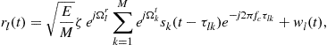
, is fixed at 20 dB. Letting ![]() go from 0 to 1, we plot the CRBs with phase errors (CRBpe) for the estimates of
go from 0 to 1, we plot the CRBs with phase errors (CRBpe) for the estimates of ![]() and
and ![]() in Figure 13.2. Note that the value of
in Figure 13.2. Note that the value of ![]() describes the severity of the phase errors, which are distributed uniformly in
describes the severity of the phase errors, which are distributed uniformly in ![]() . The corresponding coherent (CRBcoh) and noncoherent (CRBnc) CRBs without phase errors were plotted in the same figure using the results in [20].
. The corresponding coherent (CRBcoh) and noncoherent (CRBnc) CRBs without phase errors were plotted in the same figure using the results in [20].
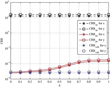
Figure 13.2 CRB for target localization versus ![]() , where the phase errors are uniformly distributed in
, where the phase errors are uniformly distributed in ![]() .
.
The figure indicates that a certain amount of phase error is tolerable if we are willing to accept a certain amount of loss. For a given acceptable loss, Figure 13.2 gives the tolerable phase errors. It is observed that CRBpe approaches CRBcoh as ![]() goes to zero, and deviates away from CRBcoh as
goes to zero, and deviates away from CRBcoh as ![]() increases. In the worst case (
increases. In the worst case (![]() ), CRBpe is approximately
), CRBpe is approximately ![]() times worse than CRBcoh, but is still approximately
times worse than CRBcoh, but is still approximately ![]() times better than CRBnc. The degradation due to the loss of knowing phase is much smaller than the degradation caused by using noncoherent processing. These results document that having noisy phase measurements is different from, and better than, not having any phase measurements.
times better than CRBnc. The degradation due to the loss of knowing phase is much smaller than the degradation caused by using noncoherent processing. These results document that having noisy phase measurements is different from, and better than, not having any phase measurements.
This is a representative example (we have tested other examples and obtained similar results) for cases with small ![]() and
and ![]() . We noted that cases with large
. We noted that cases with large ![]() and
and ![]() will also exhibit very small degradations due to phase errors since, as shown in [24], the noncoherent estimates must be perfect as
will also exhibit very small degradations due to phase errors since, as shown in [24], the noncoherent estimates must be perfect as ![]() .
.
2.13.3 Noncoherent MIMO radar
In the previous section, we discussed coherent MIMO radar with widely separated antennas, where the target reflections follow a coherent model and coherent processing is employed. Now we define a different system, called noncoherent MIMO radar, employing a noncoherent processing of received signals obeying a noncoherent target reflection model. For noncoherent MIMO radar, the antennas are separated widely enough such that they fall in different target beamwidths and the effective target reflection coefficients for different paths are distinct (which implies a noncoherent target reflection model). An example of such a case is illustrated in Figure 13.3. Denote the complex Gaussian reflection coefficient for the ![]() th path by
th path by ![]() . The received signal at receive antenna
. The received signal at receive antenna ![]() is modeled as
is modeled as
 (13.44)
where ![]() denotes the noise at receiver
denotes the noise at receiver ![]() . The simplification in going from the first to the second line in (13.44) follows since the distributions of
. The simplification in going from the first to the second line in (13.44) follows since the distributions of ![]() and
and ![]() are identical. The vector that contains all the received signals can be expressed as
are identical. The vector that contains all the received signals can be expressed as
![]() (13.45)
(13.45)
where the clutter-plus-noise vector ![]() is assumed to be zero mean Gaussian and satisfy
is assumed to be zero mean Gaussian and satisfy ![]() . The reflection coefficient vector
. The reflection coefficient vector
![]() (13.46)
(13.46)
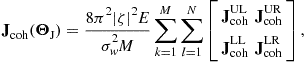
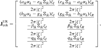
is a complex Gaussian random vector, where ![]() . Assume the matrices
. Assume the matrices ![]() and
and ![]() are both known, possibly from the pre-processing stage (e.g., the detection stage) or an adaptive procedure.6 For notational simplicity, we further assume that
are both known, possibly from the pre-processing stage (e.g., the detection stage) or an adaptive procedure.6 For notational simplicity, we further assume that ![]() has zero mean. The matrix
has zero mean. The matrix ![]() in (13.45) has the same form as (13.7) with
in (13.45) has the same form as (13.7) with ![]() . However, in this case, the
. However, in this case, the ![]() has a different definition, which is given by
has a different definition, which is given by
![]()

Figure 13.3 A noncoherent MIMO radar system with three antennas each lying in a different target beamwidth.
2.13.3.1 Joint location and velocity estimation
Similar to the discussion in Section 2.13.2.1, suppose the observed signal vector ![]() , a realization of the
, a realization of the ![]() in (13.45), is available. Our goal is to obtain the ML estimates of the target location and velocity based on the knowledge of
in (13.45), is available. Our goal is to obtain the ML estimates of the target location and velocity based on the knowledge of ![]() . Using the signal model in (13.45), the likelihood ratio with respect to
. Using the signal model in (13.45), the likelihood ratio with respect to ![]() conditioned on the reflection coefficient
conditioned on the reflection coefficient ![]() can be derived
can be derived
 (13.47)
where ![]() is a constant not dependent on
is a constant not dependent on ![]() . In (13.47),
. In (13.47), ![]() and
and ![]() , where the integral over time operates on each element of the corresponding matrix. Employing the probability density function (pdf) of the reflection coefficient
, where the integral over time operates on each element of the corresponding matrix. Employing the probability density function (pdf) of the reflection coefficient
![]() (13.48)
(13.48)
to average ![]() out, we find the likelihood ratio as a function of the unknown parameter
out, we find the likelihood ratio as a function of the unknown parameter ![]()
 (13.49)
where ![]() is a constant not dependent on
is a constant not dependent on ![]() implies the multidimensional integral over all possible values of
implies the multidimensional integral over all possible values of ![]() , and
, and
![]() (13.50)
(13.50)
In the calculations, we have assumed that the matrices ![]() ,
, ![]() , and
, and ![]() have full rank, and are hence invertible. Note that the invertibility of
have full rank, and are hence invertible. Note that the invertibility of ![]() is reasonable for MIMO radar with widely spread antennas and a target composed of a large number of scatters [5]. Further, due to thermal noise,
is reasonable for MIMO radar with widely spread antennas and a target composed of a large number of scatters [5]. Further, due to thermal noise, ![]() is also likely a full-rank matrix. From (13.49), the log-likelihood ratio can be expressed as
is also likely a full-rank matrix. From (13.49), the log-likelihood ratio can be expressed as
 (13.51)
Thus, the ML estimate of the unknown parameter vector ![]() is
is
 (13.52)
Next we employ some simplifying assumptions,7 which are quite reasonable for cases with widely spaced antennas, which simplify matters.
Assumption 3
Assume that the reflection coefficients for different paths![]() ,
,![]() are independent, such that the covariance matrix of
are independent, such that the covariance matrix of![]() is diagonal, i.e.,
is diagonal, i.e.,
![]() (13.53)
(13.53)
where![]() represents the variance of
represents the variance of![]() .
.
Consider the case where Assumptions 1–3 hold true. Thus, ![]() , and the log-likelihood ratio in (13.51) is reduced to
, and the log-likelihood ratio in (13.51) is reduced to
 (13.54)
where
![]() (13.55)
(13.55)
In (13.55), ![]() is a constant not dependent on
is a constant not dependent on ![]() and
and ![]() represents the observed signal corresponding to the
represents the observed signal corresponding to the ![]() th path, which is modeled as
th path, which is modeled as
![]() (13.56)
(13.56)
Accordingly, the ML estimate can be reduced to
 (13.57)
Unlike (13.22), in the estimator from (13.57), the squared magnitude is taken before the summation. Thus, these terms will always add in phase and so we do not need all transmitters and receivers to be synchronized in phase. Therefore, this is a noncoherent processing (across sensors). Note that under Assumptions 1–3, the noncoherent processing is optimal for the noncoherent target reflection model in Figure 13.3.
Having obtained the ML estimate for the joint location and velocity estimation, let us introduce a theorem that shows how the number of antennas affects the estimation performance.
Theorem 1
For a MIMO radar equipped with![]() transmit and
transmit and![]() receive antennas
receive antennas![]() under Assumptions 1–3 and assume that the observations follow the assumed model in (13.56), the ML estimate as described in (13.57)converges almost surely to the true parameter value when
under Assumptions 1–3 and assume that the observations follow the assumed model in (13.56), the ML estimate as described in (13.57)converges almost surely to the true parameter value when![]() is sufficiently large
is sufficiently large
![]() (13.58)
(13.58)
It follows that the ML estimate is asymptotically (![]() ) unbiased and its variance must asymptotically approach the CRB as
) unbiased and its variance must asymptotically approach the CRB as![]() .
.
This theorem indicates that increasing the number of antennas properly can improve the estimation performance of noncoherent MIMO radar. Interested readers are referred to [24] for a proof of this theorem.
To evaluate the estimation performance of noncoherent MIMO radar, in the sequel, we develop the CRBs for the joint location and velocity estimation assuming that Assumptions 1–3 hold true. The first step in obtaining the Cramer-Rao bound is to compute the FIM, which is a four-dimensional matrix related to the second order derivatives of the log-likelihood ratio in (13.54)[15]
![]()
After lengthy algebraic manipulations, following the steps similar to those in Section 2.13.2, the expression of the FIM can be obtained as below [24]:
 (13.59)
where ![]() ,
,
![]() (13.60)
(13.60)
![]() (13.61)
(13.61)
and
![]() (13.62)
(13.62)
with ![]() representing the Fourier transform of
representing the Fourier transform of ![]() . Thus, the Cramer-Rao bounds for the estimates of the unknown parameters can be determined by the diagonal elements of the inverse of the FIM as follows:
. Thus, the Cramer-Rao bounds for the estimates of the unknown parameters can be determined by the diagonal elements of the inverse of the FIM as follows:

Note that for any non-singular FIM, a closed-form expression for the Cramer-Rao bound can be easily obtained, since the analytical form of ![]() can be derived from (13.71) using Cramer’s rule.
can be derived from (13.71) using Cramer’s rule.
Example
Consider a noncoherent MIMO radar that has ![]() transmitters and
transmitters and ![]() receivers. The distance between each antenna and the origin is 7000 m. If the angles are measured with respect to the horizontal axis, then the transmitters are assumed to be uniformly distributed in
receivers. The distance between each antenna and the origin is 7000 m. If the angles are measured with respect to the horizontal axis, then the transmitters are assumed to be uniformly distributed in ![]() , where the angle of the
, where the angle of the ![]() th transmitter is
th transmitter is ![]() . The receivers are also assumed to be uniformly distributed in
. The receivers are also assumed to be uniformly distributed in ![]() , where the angle of the
, where the angle of the ![]() th receiver is
th receiver is ![]() ,
, ![]() . Assume the lowpass equivalents of the transmitted waveforms are frequency spread single Gaussian pulse signals
. Assume the lowpass equivalents of the transmitted waveforms are frequency spread single Gaussian pulse signals
 (13.63)
where ![]() is proportional to the pulse width and
is proportional to the pulse width and ![]() is the frequency increment between
is the frequency increment between ![]() and
and ![]() . We choose
. We choose ![]() kHz, and set the carrier frequency to
kHz, and set the carrier frequency to ![]() GHz. Suppose a target moving with velocity
GHz. Suppose a target moving with velocity ![]() m/s is present at
m/s is present at ![]() m. Assume the variance of each target reflection is the same for every path so that
m. Assume the variance of each target reflection is the same for every path so that ![]() . The SCNR is defined as
. The SCNR is defined as ![]() .
.
Under Assumptions 1–3, the CRB and the MSE curves of the joint ML estimates are plotted versus SCNR in Figure 13.4 for the MIMO radar system with ![]() transmitters and
transmitters and ![]() receivers. It is observed from the simulation results that the MSEs of the ML estimates approach the corresponding CRBs as the SCNR becomes large. This is consistent with the theoretical asymptotic efficiency of ML estimates and also corroborates the correctness of the derived CRBs presented earlier.
receivers. It is observed from the simulation results that the MSEs of the ML estimates approach the corresponding CRBs as the SCNR becomes large. This is consistent with the theoretical asymptotic efficiency of ML estimates and also corroborates the correctness of the derived CRBs presented earlier.

The curves for a noncoherent MIMO radar with ![]() transmitters and
transmitters and ![]() receivers are plotted in Figure 13.5. Compared with Figure 13.4, it is seen that increasing the number of antennas decreases the CRB uniformly and lowers the threshold (i.e., the SCNR at which the MSE curve changes slope drastically, see arrows in the figure) to a smaller value. We also find that these MSE curves get more favorable (closer to CRB in the asymptotic region) with more antennas. These results show that more antennas means better performance in both asymptotic (large
receivers are plotted in Figure 13.5. Compared with Figure 13.4, it is seen that increasing the number of antennas decreases the CRB uniformly and lowers the threshold (i.e., the SCNR at which the MSE curve changes slope drastically, see arrows in the figure) to a smaller value. We also find that these MSE curves get more favorable (closer to CRB in the asymptotic region) with more antennas. These results show that more antennas means better performance in both asymptotic (large ![]() ) and non-asymptotic cases.
) and non-asymptotic cases.

Figure 13.5 MSE versus SCNR for the ![]() noncoherent MIMO radar with transmit antennas placed uniformly in
noncoherent MIMO radar with transmit antennas placed uniformly in ![]() and receive antennas also placed uniformly in
and receive antennas also placed uniformly in ![]() .
.
More explorations on the noncoherent MIMO radar joint location and velocity estimation are presented in [24], which include the analyses on the threshold phenomenon, the impact of finite system resources, the effects of changing antenna placement, the effects of employing different waveforms, and the noncoherent ambiguity function. Extensions to several general cases, such as for dependent reflection coefficients, nonorthogonal signals, and for spatially colored clutter-plus-noise, are also provided in [24].
2.13.3.2 Noncoherent ambiguity function
Having studied the CRB, we now consider the ambiguity function (AF) for noncoherent MIMO radar. Under Assumptions 1–3, the noncoherent AF has been developed in [24] in two different ways yielding
 (13.64)
where ![]() , with
, with ![]() determined by the antenna positions which can be obtained by substituting
determined by the antenna positions which can be obtained by substituting ![]() into (13.2). Note that since the
into (13.2). Note that since the ![]() and
and ![]() in (13.64) are functions of
in (13.64) are functions of ![]() and
and ![]() , respectively, the AF is essentially a four-dimensional function with respect to variables
, respectively, the AF is essentially a four-dimensional function with respect to variables ![]() . Interested readers are referred to [24] for more detailed derivations.
. Interested readers are referred to [24] for more detailed derivations.
Example
Consider a noncoherent MIMO radar system with ![]() transmit and
transmit and ![]() receive antennas uniformly placed in direction
receive antennas uniformly placed in direction ![]() , where the look angles are
, where the look angles are ![]() and
and ![]() . To make the AF a simple two-dimensional function that we can plot and easily interpret, we assume the target only move along the
. To make the AF a simple two-dimensional function that we can plot and easily interpret, we assume the target only move along the ![]() -axis such that
-axis such that ![]() . Further assume that the monitored area is relatively small and all antennas are located sufficiently far away, so that the
. Further assume that the monitored area is relatively small and all antennas are located sufficiently far away, so that the ![]() and
and ![]() can be approved to be approximately linearly related to
can be approved to be approximately linearly related to ![]() and
and ![]() through
through
![]() (13.65)
(13.65)
![]() (13.66)
(13.66)
Thus, the noncoherent AF from (13.64) can be simplified to
 (13.67)
Assume frequency spread single Gaussian pulse signals are used for transmission, whose complex envelopes ![]() are given in (13.63). Plugging
are given in (13.63). Plugging ![]() into (13.67), the simplified noncoherent AF for the single Gaussian pulse can be obtained
into (13.67), the simplified noncoherent AF for the single Gaussian pulse can be obtained
The AFs of noncoherent MIMO radar systems with different configurations are plotted in Figure 13.6. The system considered in Figure 13.6a has ![]() transmitters and
transmitters and ![]() receivers, while the system considered in Figure 13.6b has
receivers, while the system considered in Figure 13.6b has ![]() transmitters and
transmitters and ![]() receivers. Using the previously defined simplified AF for the specific examples under study, it can be seen that the mainlobe of AF becomes narrower as more antennas are added. This is easier to read in the
receivers. Using the previously defined simplified AF for the specific examples under study, it can be seen that the mainlobe of AF becomes narrower as more antennas are added. This is easier to read in the ![]() -level contour plots shown in Figure 13.6c. Narrower AF means better resolution, thus the performance is improved by using more antennas in this example.
-level contour plots shown in Figure 13.6c. Narrower AF means better resolution, thus the performance is improved by using more antennas in this example.
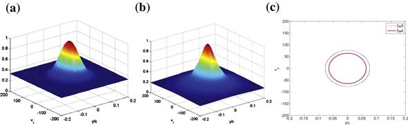
Figure 13.6 AF of noncoherent MIMO radar systems transmitting frequency spread single Gaussian pulse signals with (a) ![]() , (b)
, (b) ![]() antennas, and their (c)
antennas, and their (c) ![]() -level contour, assuming that
-level contour, assuming that ![]() .
.
Assume frequency spread Gaussian pulse trains are used for transmission, thus the signal transmitted from the ![]() th transmitter is
th transmitter is
![]() (13.68)
(13.68)
where ![]() is the pulse repetition interval,
is the pulse repetition interval, ![]() the narrow Gaussian pulse with pulsewidth
the narrow Gaussian pulse with pulsewidth ![]() the broad Gaussian envelope with pulsewidth
the broad Gaussian envelope with pulsewidth ![]() , and
, and ![]() the frequency increment. Plugging
the frequency increment. Plugging ![]() into (13.67) gives the simplified noncoherent AF for the Gaussian pulse train
into (13.67) gives the simplified noncoherent AF for the Gaussian pulse train

The AF for the noncoherent MIMO radar system with 5 transmitters and 4 receivers is plotted in Figure 13.7a, while the AF for the noncoherent MIMO radar system with 9 transmitters and 9 receivers is plotted in Figure 13.7b. We see that ambiguity sidelobes are created by the use of the Gaussian pulse train. Comparing Figure 13.7b to a, it is seen that when the number of antennas increases, the sidelobes decease for the example considered here and our simplified AF. Again, these examples illustrate that using more antennas can give a better AF for noncoherent MIMO radar.

2.13.4 Performance and complexity analysis for coherent and noncoherent MIMO radar
In the previous sections, we have introduced the coherent and noncoherent MIMO radar systems and investigated their joint target location and velocity estimation abilities. The characteristics of the coherent and noncoherent MIMO radar merit more discussions. As opposed to the noncoherent counterpart, the coherent MIMO radar requires extra phase synchronization, which may not be very amenable to practical implementation. Aiming to identify possible scenarios that enable us to replace the coherent MIMO radar with the easier-to-implement noncoherent one but without inducing much loss in performance, we devote this section to studying the MSE performance difference between these two approaches.
It was indicated in [11] that when target localization is the application of interest, significant gains can be obtained through the use of coherent MIMO radar, over noncoherent radar. Here we will demonstrate that the magnitude of these gains decreases with an increase in the product of the number of transmit and receive antennas. In particular, the performance of the noncoherent MIMO radar approaches that of the coherent MIMO radar when the product of the number of transmit and receive antennas is sufficiently large.
2.13.4.1 Normalized mean square error difference
Let ![]() and
and ![]() denote the actual and estimated value of the parameter vector to be estimated
denote the actual and estimated value of the parameter vector to be estimated ![]() . Define the total MSE of the joint estimation as
. Define the total MSE of the joint estimation as
 (13.69)
where ![]() defines a constant weighting vector with the same length as
defines a constant weighting vector with the same length as ![]() and
and ![]() represents the MSE corresponding to the
represents the MSE corresponding to the ![]() th component of
th component of ![]() (i.e.,
(i.e., ![]() ). Note here we consider a weighted MSE that allows one to give extra priority to some components over others. Of course, taking the weight as a constant vector is also possible, which gives equal weight to all the components.
). Note here we consider a weighted MSE that allows one to give extra priority to some components over others. Of course, taking the weight as a constant vector is also possible, which gives equal weight to all the components.
Theorem 1
Consider a MIMO radar equipped with![]() separated transmit antennas and
separated transmit antennas and![]() separated receive antennas for joint location and velocity estimation. Assume the coherent MIMO radar (13.22)performs better (in the sense of leading to a smaller MSE
separated receive antennas for joint location and velocity estimation. Assume the coherent MIMO radar (13.22)performs better (in the sense of leading to a smaller MSE![]() than the noncoherent MIMO radar (13.57)for all
than the noncoherent MIMO radar (13.57)for all![]() and
and![]() . Under Assumptions 1 and 2, the MSE of the ML estimate for the noncoherent MIMO radar
. Under Assumptions 1 and 2, the MSE of the ML estimate for the noncoherent MIMO radar![]() gets as close as desired to that of the coherent MIMO radar
gets as close as desired to that of the coherent MIMO radar![]() for sufficiently large
for sufficiently large![]() .
.
For a detailed proof of the theorem, please refer to [16].
Remark 1
Theorem 1 implies that under the given assumptions, the noncoherent MIMO radar, which has less stringent synchronization requirements, is generally more preferable than its coherent counterpart for sufficiently large ![]() . Stated a different way: (1) If the noncoherent MIMO radar leads to smaller MSE than the coherent MIMO radar, the noncoherent MIMO radar is preferred without a doubt, since it performs better and has less stringent synchronization requirements; (2) otherwise, if the coherent MIMO radar leads to smaller MSE than the noncoherent MIMO radar, as shown by Theorem 1, one can add more antennas to compensate, so that at some large
. Stated a different way: (1) If the noncoherent MIMO radar leads to smaller MSE than the coherent MIMO radar, the noncoherent MIMO radar is preferred without a doubt, since it performs better and has less stringent synchronization requirements; (2) otherwise, if the coherent MIMO radar leads to smaller MSE than the noncoherent MIMO radar, as shown by Theorem 1, one can add more antennas to compensate, so that at some large ![]() the MSE performance of the noncoherent MIMO radar is sufficiently close to that of the coherent MIMO radar and thus the noncoherent MIMO radar is good enough.
the MSE performance of the noncoherent MIMO radar is sufficiently close to that of the coherent MIMO radar and thus the noncoherent MIMO radar is good enough.
Based on the total MSEs of the joint estimation for the coherent and noncoherent MIMO radars, assuming a known constant ![]() , we define the normalized difference of the root mean square errors (NDRMSE) to evaluate the overall difference in the MSE of the coherent and noncoherent MIMO radars as below
, we define the normalized difference of the root mean square errors (NDRMSE) to evaluate the overall difference in the MSE of the coherent and noncoherent MIMO radars as below
 (13.70)
where it is assumed that ![]() . If
. If ![]() , then we would use
, then we would use ![]() directly. The smaller the
directly. The smaller the ![]() , the closer the MSE performance between the two estimators. For a predetermined value of
, the closer the MSE performance between the two estimators. For a predetermined value of ![]() , which is chosen to satisfy particular requirements, the MSE performance of the noncoherent MIMO radar is considered to be good enough if
, which is chosen to satisfy particular requirements, the MSE performance of the noncoherent MIMO radar is considered to be good enough if ![]() , and in such cases the noncoherent MIMO radar is preferred for its less stringent synchronization requirements.
, and in such cases the noncoherent MIMO radar is preferred for its less stringent synchronization requirements.
Particularly, in the joint location and velocity estimation problem discussed previously, ![]() , so we have
, so we have
 (13.71)
 (13.72)
and
 (13.73)
where it is assumed that ![]() . Note that one can easily adjust for units by proper selection of
. Note that one can easily adjust for units by proper selection of ![]() . Later in the numerical examples, we employ
. Later in the numerical examples, we employ ![]() for all
for all ![]() .
.
2.13.4.2 Numerical examples
Example 1
Consider a MIMO radar that has ![]() transmitters and
transmitters and ![]() receivers. When employing the coherent MIMO radar, the antennas are uniformly placed in
receivers. When employing the coherent MIMO radar, the antennas are uniformly placed in ![]() , where
, where ![]() and
and ![]() . In the example, Assumptions 1 and 2 are adopted. When employing the noncoherent MIMO radar, the antennas are uniformly placed in direction
. In the example, Assumptions 1 and 2 are adopted. When employing the noncoherent MIMO radar, the antennas are uniformly placed in direction ![]() , where the angle of transmitter
, where the angle of transmitter ![]() with respect to the horizontal axis is
with respect to the horizontal axis is ![]() and the angle of receiver
and the angle of receiver ![]() is
is ![]() ,
, ![]() . Let
. Let ![]() kHz, such that
kHz, such that ![]() , and thus the transmitted signals are approximately orthogonal ([24]). Assume the SCNR is 20 dB.
, and thus the transmitted signals are approximately orthogonal ([24]). Assume the SCNR is 20 dB.
Suppose the system resources employed were not considered, the energy assigned to each transmit antenna was fixed, so adding a transmit antenna implies an extra energy source and increased total transmitted energy. In this case, the NDRMSEs are plotted versus ![]() with
with ![]() (or
(or ![]() ) going from 1 to 20 for a fixed
) going from 1 to 20 for a fixed ![]() (or
(or ![]() ) in Figure 13.8a. It is observed that increasing either
) in Figure 13.8a. It is observed that increasing either ![]() or
or ![]() decreases the NDRMSE, which makes the MSE performance of the noncoherent MIMO radar get closer to that of the coherent MIMO radar. When the system resources employed are taken into account, the situation becomes complicated. In such cases, the total transmitted energy is fixed, so that adding transmit antennas means splitting the energy over more antennas. Figure 13.8b shows such an example. Under the energy constraint, the NDRMSEs are plotted versus
decreases the NDRMSE, which makes the MSE performance of the noncoherent MIMO radar get closer to that of the coherent MIMO radar. When the system resources employed are taken into account, the situation becomes complicated. In such cases, the total transmitted energy is fixed, so that adding transmit antennas means splitting the energy over more antennas. Figure 13.8b shows such an example. Under the energy constraint, the NDRMSEs are plotted versus ![]() with the other parameters set the same as Figure 13.8a. It is observed that, when the total energy is fixed, increasing the number of receive antennas
with the other parameters set the same as Figure 13.8a. It is observed that, when the total energy is fixed, increasing the number of receive antennas ![]() always decreases NDRMSE, but this is not true when we increase the number of transmit antennas
always decreases NDRMSE, but this is not true when we increase the number of transmit antennas ![]() for a fixed
for a fixed ![]() . Increasing
. Increasing ![]() first decreases the NDRMSE (when
first decreases the NDRMSE (when ![]() is small, e.g.,
is small, e.g., ![]() in this example), but later increases the NDRMSE when
in this example), but later increases the NDRMSE when ![]() is large (e.g.,
is large (e.g., ![]() in this example). Here we see the effects of spreading the energy too thinly between the transmit antennas. This occurs when
in this example). Here we see the effects of spreading the energy too thinly between the transmit antennas. This occurs when ![]() is too large.
is too large.

2.13.4.2.1 Example 2
Consider the same scenario in Figure 13.8, except that the antenna positions for the noncoherent MIMO radar are different. Here the transmit antennas are assumed to be at ![]() m,
m, ![]() and the receive antennas are assumed to be at
and the receive antennas are assumed to be at ![]() m,
m, ![]() . In this example, we fix the total number of antennas to
. In this example, we fix the total number of antennas to ![]() . This is an approximate way to fix the total system complexity, since each added antenna implies the addition of several accompanying hardware components. Further, counting system complexity through the total number of antennas used can obviate the need for getting involved with details related to the hardware implementation. This is very useful in a high level study like the one we undertake here.
. This is an approximate way to fix the total system complexity, since each added antenna implies the addition of several accompanying hardware components. Further, counting system complexity through the total number of antennas used can obviate the need for getting involved with details related to the hardware implementation. This is very useful in a high level study like the one we undertake here.
When the energy is unconstrained, i.e., the transmit energy per transmit antenna is fixed so that adding a transmit antenna increases the total transmit energy, the RMSEis are plotted in Figure 13.9a. It is seen that there is a symmetry between ![]() and
and ![]() , and the minima for both the coherent and noncoherent MIMO radars occur at
, and the minima for both the coherent and noncoherent MIMO radars occur at ![]() , as expected. When the total energy is constrained, i.e., adding a transmit antenna decreases the transmit energy per transmit antenna, the RMSEis are plotted in Figure 13.9b. It is seen that the effects of increasing
, as expected. When the total energy is constrained, i.e., adding a transmit antenna decreases the transmit energy per transmit antenna, the RMSEis are plotted in Figure 13.9b. It is seen that the effects of increasing ![]() and
and ![]() are asymmetric. For both the coherent and noncoherent MIMO radars,
are asymmetric. For both the coherent and noncoherent MIMO radars, ![]() is the best, and further increasing
is the best, and further increasing ![]() will degrade the performance. The NDRMSEs for the unconstrained and constrained energy cases are plotted versus
will degrade the performance. The NDRMSEs for the unconstrained and constrained energy cases are plotted versus ![]() in Figure 13.9c and d, respectively. The best MSE performance occurs at
in Figure 13.9c and d, respectively. The best MSE performance occurs at ![]() for the unconstrained case and for an
for the unconstrained case and for an ![]() such that
such that ![]() for the constrained case. In fact we have tested other cases (different placements and fixed
for the constrained case. In fact we have tested other cases (different placements and fixed ![]() value) and obtained similar results.
value) and obtained similar results.
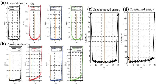
Figure 13.9 ![]() ’s (in m for location and m/s for velocity) for the joint estimation of location and velocity with (a) unconstrained energy or (b) constrained energy, and the corresponding NDRMSEs (c)–(d) versus
’s (in m for location and m/s for velocity) for the joint estimation of location and velocity with (a) unconstrained energy or (b) constrained energy, and the corresponding NDRMSEs (c)–(d) versus ![]() .
. ![]() . SCNR = 20 dB.
. SCNR = 20 dB.
The main point is that if we fix the total energy and if we add too many transmit antennas then we will spread the energy too thinly among the transmit antennas and this will lead to bad performance. On the other hand, there are cases where we get gains from adding transmit antennas with fixed total energy, for example, when we do not spread the energy too thinly. Usually, it is better to use more than one transmit antenna to obtain good performance. Further numerical investigations and discussions can be found in [16].
2.13.5 Diversity gain for MIMO radar Neyman-Pearson signal detection
So far, the chapter has been about MIMO radar for estimation. In this section, we discuss the diversity gain that a MIMO radar system can render in the context of target detection. Diversity gain is one significant advantage that MIMO radar systems employing separated antennas can bring forth when compared with more traditional radar systems. When the Neyman-Pearson criterion is employed, for a fixed false alarm probability, diversity gain is defined as the negative of the slope of the miss probability versus SCNR for the high SCNR region when a logarithmic scale is employed for both axes. Assuming linear decay of the miss probability for sufficiently large SCNR when such scales are employed, large diversity gain implies good target detection performance for sufficiently high SCNR and fixed probability of false alarm. If we have two detectors and one has larger diversity gain, then at some sufficiently large SCNR, the detector with larger diversity gain must have smaller miss probability. Intuitively, diversity gain tells us about the value of the information we get from multiple looks (from several antennas, frequencies, or retransmissions, etc.).
2.13.5.1 Signal model
Consider a radar system that has ![]() transmit and
transmit and ![]() receive antennas. The positions of the transmit and receive antennas of the radar system are
receive antennas. The positions of the transmit and receive antennas of the radar system are ![]() and
and ![]() , respectively. Denote the waveform transmitted by the
, respectively. Denote the waveform transmitted by the ![]() th antenna by
th antenna by ![]() , where
, where ![]() and
and ![]() can be non-orthogonal for
can be non-orthogonal for ![]() , in the sense of [4]. Assume each waveform is normalized to give transmitted power
, in the sense of [4]. Assume each waveform is normalized to give transmitted power ![]() . The radar will break up the monitored space into cells and sequentially probe each cell for a target. Thus, our goal is to find out whether a target is at a particular position or not. Assume a target, if present, is composed of
. The radar will break up the monitored space into cells and sequentially probe each cell for a target. Thus, our goal is to find out whether a target is at a particular position or not. Assume a target, if present, is composed of ![]() point scatterers, located at
point scatterers, located at ![]() . The reflection coefficient,
. The reflection coefficient, ![]() for the
for the ![]() th scatterer, is assumed to be constant over the observation interval.
th scatterer, is assumed to be constant over the observation interval.
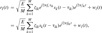
The clutter-plus-noise-free received signal at receive antenna ![]() due to the transmission from transmit antenna
due to the transmission from transmit antenna ![]() and the reflection from the
and the reflection from the ![]() th scatterer is modeled as [4]
th scatterer is modeled as [4]
![]() (13.74)
(13.74)
where ![]() denotes the time delay from transmit antenna
denotes the time delay from transmit antenna ![]() to receive antenna
to receive antenna ![]() due to the reflection from the
due to the reflection from the ![]() th scatterer,
th scatterer, ![]() , and
, and ![]() is the speed of light. Assume the transmitted waveforms are relatively narrow band, where the bandwidth of the waveforms is given such that they are not capable of resolving individual scatterers [5]. Therefore,
is the speed of light. Assume the transmitted waveforms are relatively narrow band, where the bandwidth of the waveforms is given such that they are not capable of resolving individual scatterers [5]. Therefore,
![]() (13.75)
(13.75)
where ![]() denotes the time delay from a reflection off a scatterer located at the gravity center of the scatterers
denotes the time delay from a reflection off a scatterer located at the gravity center of the scatterers ![]() . Then (13.74) can be written as
. Then (13.74) can be written as
![]() (13.76)
(13.76)
Thus, the received signal at receive antenna ![]() due to the propagation from all
due to the propagation from all ![]() transmit antennas and all
transmit antennas and all ![]() scatterers is given by
scatterers is given by
 (13.77)
where ![]() denotes the clutter-plus-noise observed at the
denotes the clutter-plus-noise observed at the ![]() th receiver.
th receiver.
2.13.5.2 Effect of signal space dimension on diversity gain
Suppose we attempt to implement the optimum receiver for the Gaussian reflection coefficients and Gaussian clutter-plus-noise case following (13.77), by first projecting the received continuous-time observations onto a basis that spans the space spanned by the first term, the signal term, in (13.77). Let the set of ![]() orthonormal basis functions
orthonormal basis functions ![]() span the
span the ![]() dimensional space spanned by the first term, the signal term, of (13.77). The expansion, in terms of this basis, of any delayed signal term appearing in (13.77) can be expressed as
dimensional space spanned by the first term, the signal term, of (13.77). The expansion, in terms of this basis, of any delayed signal term appearing in (13.77) can be expressed as
 (13.78)
with the coefficients defined by
![]() (13.79)
(13.79)
which are obtained by using (orthonormal basis)
 (13.80)
after taking the inner product with ![]() (right hand side of (13.79)) on both sides of (13.78). We note that the largest possible value of
(right hand side of (13.79)) on both sides of (13.78). We note that the largest possible value of ![]() is
is ![]() and this occurs when each of the delayed signal terms in (13.77), the terms expanded in (13.78), are linearly independent. Now we can project the received signal
and this occurs when each of the delayed signal terms in (13.77), the terms expanded in (13.78), are linearly independent. Now we can project the received signal ![]() in (13.77) onto this basis to obtain8
in (13.77) onto this basis to obtain8
 (13.81)
where ![]() , and
, and ![]() is a vector of reflection coefficients for those
is a vector of reflection coefficients for those ![]() scatterers. Collecting the
scatterers. Collecting the ![]() outputs and letting
outputs and letting ![]() , we have
, we have
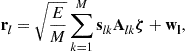 (13.82)
where
![]() (13.83)
(13.83)
and ![]() . Further, stacking the outputs across all the
. Further, stacking the outputs across all the ![]() receivers into a single vector gives
receivers into a single vector gives
 (13.84)
where
![]() (13.85)
(13.85)
denotes a block diagonal matrix with submatrices ![]() , …,
, …, ![]() on its diagonal, and the size of each submatrix
on its diagonal, and the size of each submatrix
![]() (13.86)
(13.86)
![]() (13.87)
(13.87)
then the dimension of matrix ![]() is given by
is given by ![]() . The
. The ![]() in (13.84) is an
in (13.84) is an ![]() clutter-plus-noise vector with covariance matrix
clutter-plus-noise vector with covariance matrix ![]() . Based on (13.84), we have the following results which elaborate the diversity gain offered by MIMO radar systems employing non-orthogonal waveforms.
. Based on (13.84), we have the following results which elaborate the diversity gain offered by MIMO radar systems employing non-orthogonal waveforms.
Theorem 1
Consider a MIMO radar system with![]() transmit and
transmit and![]() receive antennas and observations following (13.77)with possibly nonGaussian clutter-plus-noise and reflection coefficients. After expanding the received signals using basis functions as per (13.81)and collecting the coefficients as per (13.84), the detection system can be described by a hypothesis testing problem as follows
receive antennas and observations following (13.77)with possibly nonGaussian clutter-plus-noise and reflection coefficients. After expanding the received signals using basis functions as per (13.81)and collecting the coefficients as per (13.84), the detection system can be described by a hypothesis testing problem as follows![]()
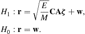 (13.88)
Assume that a detector of the class of
![]() (13.89)
(13.89)
is employed with an arbitrary![]() that meets
that meets![]() and a positive finite threshold
and a positive finite threshold![]() determined by the required false alarm probability. Plug (13.88)under
determined by the required false alarm probability. Plug (13.88)under![]() into (13.89)and write the test statistic in the form of
into (13.89)and write the test statistic in the form of
![]() (13.90)
(13.90)
to define![]() and
and![]() . If the cumulative distribution function
. If the cumulative distribution function![]() cdf
cdf![]() of
of![]() denoted as
denoted as![]() satisfies
satisfies
![]() (13.91)
(13.91)
for some constant9![]() and nonzero constant
and nonzero constant![]() and
and
![]() (13.92)
(13.92)
holds true![]() then the diversity gain achieved by this system is
then the diversity gain achieved by this system is![]() .
.
Remark 2
For the hypothesis testing problem in (13.88), if the clutter-plus-noise ![]() is zero-mean Gaussian with covariance matrix
is zero-mean Gaussian with covariance matrix ![]() and the reflection coefficient
and the reflection coefficient ![]() is zero-mean Gaussian with covariance matrix
is zero-mean Gaussian with covariance matrix ![]() , then the detector in (13.89) is optimum for
, then the detector in (13.89) is optimum for
![]() (13.93)
(13.93)
where ![]() satisfies
satisfies ![]() and
and ![]() denotes the SCNR the detector is designed for.
denotes the SCNR the detector is designed for.
Theorem 2
Consider a MIMO radar system with![]() transmit and
transmit and![]() receive antennas attempting to detect the presence of a target with
receive antennas attempting to detect the presence of a target with![]() scatterers. Assume observations following (13.77)with possibly nonGaussian clutter-plus-noise and reflection coefficients. After expanding the
scatterers. Assume observations following (13.77)with possibly nonGaussian clutter-plus-noise and reflection coefficients. After expanding the![]() -dimensional signal at the
-dimensional signal at the![]() th receive antenna
th receive antenna![]()
![]() using basis functions as per (13.81)and collecting the coefficients as per (13.84), assume that a detector of the class of (13.89)is employed, which includes the optimum detector for Gaussian clutter-plus-noise and reflections. Plug (13.88)under
using basis functions as per (13.81)and collecting the coefficients as per (13.84), assume that a detector of the class of (13.89)is employed, which includes the optimum detector for Gaussian clutter-plus-noise and reflections. Plug (13.88)under![]() into (13.89)and write the test statistic in the form of
into (13.89)and write the test statistic in the form of
 (13.94)
where![]() to define
to define![]() and
and![]() . If each
. If each![]() for
for![]() has a cdf
has a cdf![]() that satisfies
that satisfies
![]() (13.95)
(13.95)
for some constant![]() and nonzero
and nonzero![]() and (13.92)holds true
and (13.92)holds true![]() then the maximum diversity gain is
then the maximum diversity gain is
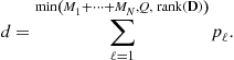 (13.96)
This maximum diversity gain can be achieved under some conditions![]() for example statistically independent
for example statistically independent![]() and
and![]() has full row or column rank.
has full row or column rank.
For the special case of Gaussian reflection coefficients (Gaussian signals), it is known from [25] that ![]() , so the diversity gain is given by
, so the diversity gain is given by ![]() . When the Gaussian optimum detector is employed, it can be shown that
. When the Gaussian optimum detector is employed, it can be shown that ![]() , which leads to a diversity gain
, which leads to a diversity gain ![]() . Further, suppose the dimension of the space spanned by the target-reflected noise-free received waveforms at different receivers are the same for all
. Further, suppose the dimension of the space spanned by the target-reflected noise-free received waveforms at different receivers are the same for all ![]() , such that
, such that ![]() . Then the largest possible diversity gain described in Theorem 2 becomes
. Then the largest possible diversity gain described in Theorem 2 becomes ![]() .
.
Assuming the number of scatterers is very large such that ![]() , Theorem 2 implies that to achieve the largest possible diversity gain,
, Theorem 2 implies that to achieve the largest possible diversity gain, ![]() , the noise-free received waveforms, due to target reflection, at the
, the noise-free received waveforms, due to target reflection, at the ![]() th receiver must span the entire
th receiver must span the entire ![]() dimensional space. If the clutter-plus-noise free received waveforms span a lower dimension, say
dimensional space. If the clutter-plus-noise free received waveforms span a lower dimension, say ![]() , the diversity gain will be equal to or smaller than
, the diversity gain will be equal to or smaller than ![]() , which is less than
, which is less than ![]() in this case. In other words, MIMO radars that employ either orthogonal waveforms or non-orthogonal waveforms can provide the maximum achievable diversity gain, as long as the noise-free received waveforms, due to target reflection, at each receiver span an
in this case. In other words, MIMO radars that employ either orthogonal waveforms or non-orthogonal waveforms can provide the maximum achievable diversity gain, as long as the noise-free received waveforms, due to target reflection, at each receiver span an ![]() dimensional space.
dimensional space.
Example 1
Consider a MIMO radar system that has ![]() transmit antennas located at
transmit antennas located at ![]() km and
km and ![]() km, and
km, and ![]() receive antennas located at
receive antennas located at ![]() km and
km and ![]() km. The waveforms emitted from these two transmitters are
km. The waveforms emitted from these two transmitters are ![]() and
and ![]() respectively. Gaussian optimum detector is employed. Assume the
respectively. Gaussian optimum detector is employed. Assume the ![]() scatterers constituting the target are uniformly distributed over [0.3, 1] × [9.4, 10.5] km2. Each scatterer has a statistically independent scattering coefficient. In each example, the probability of miss versus SCNR curve is obtained from
scatterers constituting the target are uniformly distributed over [0.3, 1] × [9.4, 10.5] km2. Each scatterer has a statistically independent scattering coefficient. In each example, the probability of miss versus SCNR curve is obtained from ![]() Monte Carlo simulations per SCNR, and the resulting diversity gains are compared with those calculated using the corresponding theorem from the previous sections.
Monte Carlo simulations per SCNR, and the resulting diversity gains are compared with those calculated using the corresponding theorem from the previous sections.
Assume the reflection coefficients and the clutter-plus-noise are statistically independent complex Gaussian with zero mean. Assume the noise-free received waveforms (due to target reflection) at each receiver, ![]() and
and ![]() , are normalized and orthogonal [4]. In this case, these waveforms themselves are the orthonormal basis functions,
, are normalized and orthogonal [4]. In this case, these waveforms themselves are the orthonormal basis functions, ![]() and
and ![]() , such that
, such that ![]() ,
, ![]() , and
, and ![]() as per (13.83), and the
as per (13.83), and the ![]() in (13.86) is a
in (13.86) is a ![]() identity matrix, for
identity matrix, for ![]() . Therefore the matrix
. Therefore the matrix ![]() in (13.85) is a
in (13.85) is a ![]() identity matrix and
identity matrix and ![]() . Further, assume the number of scatterers is
. Further, assume the number of scatterers is ![]() . When the probability of false alarm is fixed at
. When the probability of false alarm is fixed at ![]() , the probability of miss detection
, the probability of miss detection ![]() is plotted versus SCNR in the solid curve with points marked with squares in Figure 13.10. It is seen that increasing SCNR by 10 dB decreases the
is plotted versus SCNR in the solid curve with points marked with squares in Figure 13.10. It is seen that increasing SCNR by 10 dB decreases the ![]() by four decades approximately. Thus, the slope of the miss probability versus SCNR, if plotted on a log-log scale, is approximately
by four decades approximately. Thus, the slope of the miss probability versus SCNR, if plotted on a log-log scale, is approximately ![]() . This agrees well with Theorem 2, where the maximum diversity gain is
. This agrees well with Theorem 2, where the maximum diversity gain is ![]() , recalling that
, recalling that ![]() for Gaussian reflections. Note that in this example
for Gaussian reflections. Note that in this example ![]() , the maximum diversity gain is achieved as expected, which is guaranteed by the statistically independent reflections of the
, the maximum diversity gain is achieved as expected, which is guaranteed by the statistically independent reflections of the ![]() scatterers, according to the discussion after Theorem 2.
scatterers, according to the discussion after Theorem 2.
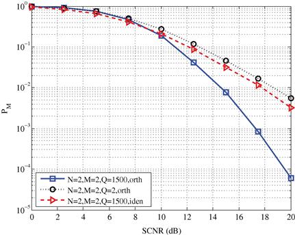
Figure 13.10 Probability of miss versus SCNR for three difference cases under the condition of Gaussian reflections and Gaussian clutter-plus-noise.
In the second example, we assume the number of scatterers constituting the target is reduced to ![]() . The other parameters are kept unchanged. The
. The other parameters are kept unchanged. The ![]() versus SCNR is shown in the dotted curve with points marked with circles in Figure 13.10. It is observed that increasing SCNR by
versus SCNR is shown in the dotted curve with points marked with circles in Figure 13.10. It is observed that increasing SCNR by ![]() decreases the
decreases the ![]() by two decades approximately. The slope of the decrease of the miss probability versus SCNR on a log-log scale is thereby
by two decades approximately. The slope of the decrease of the miss probability versus SCNR on a log-log scale is thereby ![]() . This also justifies Theorem 2, where the maximum diversity gain is
. This also justifies Theorem 2, where the maximum diversity gain is ![]() .
.
The third example considers the same scenario as the first example, except that we assume the two noise-free received waveforms at each receiver (due to target reflection) are identical, ![]() , where
, where ![]() . Thus,
. Thus, ![]() and
and ![]() , and
, and ![]() . Hence, the matrix
. Hence, the matrix ![]() in (13.85) is a
in (13.85) is a ![]() matrix, and
matrix, and ![]() . In this case,
. In this case, ![]() versus SCNR is plotted in the dashed curve with points marked with triangles in Figure 13.10. It is seen that the diversity gain is approximately
versus SCNR is plotted in the dashed curve with points marked with triangles in Figure 13.10. It is seen that the diversity gain is approximately ![]() . Again, Theorem 2 is justified, since the maximum diversity gain
. Again, Theorem 2 is justified, since the maximum diversity gain ![]() . This example illustrates the importance of the signal space spanned by the received waveforms.
. This example illustrates the importance of the signal space spanned by the received waveforms.
Example 2
This numerical example illustrates the maximum diversity gains that can be achieved by the MIMO radar system employing orthogonal waveforms and the traditional phased array radar system. We focus on Gaussian signals and clutter-plus-noise. Employ the test in (13.89) with ![]() which we call noncoherent MIMO radar employing orthogonal waveforms (which maintain orthogonality after each experiencing different delays) [2], and
which we call noncoherent MIMO radar employing orthogonal waveforms (which maintain orthogonality after each experiencing different delays) [2], and ![]() which we call coherent processing. The resulting
which we call coherent processing. The resulting ![]() versus SCNR curves are shown in Figure 13.11. It is found that, for the noncoherent processing (solid curve with triangles), increasing SCNR by
versus SCNR curves are shown in Figure 13.11. It is found that, for the noncoherent processing (solid curve with triangles), increasing SCNR by ![]() dB approximately decreases the
dB approximately decreases the ![]() by four decades, so that
by four decades, so that ![]() , which justifies
, which justifies ![]() for the noncoherent MIMO radar employing orthogonal waveforms. On the other hand, for the coherent processing (dashed curve with diamonds) used in the phased array radar, increasing SCNR by
for the noncoherent MIMO radar employing orthogonal waveforms. On the other hand, for the coherent processing (dashed curve with diamonds) used in the phased array radar, increasing SCNR by ![]() dB approximately decreases the
dB approximately decreases the ![]() by one decade so that
by one decade so that ![]() , which justifies
, which justifies ![]() for the phased array radar performing beamforming.
for the phased array radar performing beamforming.
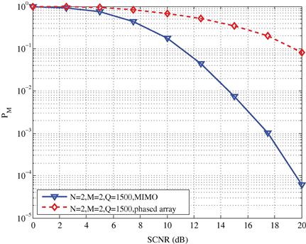
For more theoretical analysis and numerical examples on non-Gaussian signals and non-Gaussian clutter-plus-noise, please refer to [25].
2.13.6 Phase synchronization for coherent MIMO radar
In the previous sections, we have elucidated the characteristics of both coherent MIMO radar and noncoherent MIMO radar. Regardless of which mode is employed, all the elements10 in MIMO radar need to synchronize firstly in terms of, for example, time, frequency, or phase. In fact, phase synchronization embodies a major difference between the operations of noncoherent MIMO radar and coherent MIMO radar: the coherent approach requires phase synchronization between the separated antenna elements, while the noncoherent counterpart does not. Note that in reality, MIMO radar elements are usually operated with physically different local oscillators, and each of them suffers from statistically independent phase offset, indicating that the phase of the carrier signal transmitted gets rotated by an unknown amount. Such imperfection in phase coherence can have an unfavorable effect on the performance of coherent MIMO radar, e.g., [26–29]. As a result, practical implementation of coherent MIMO radar systems needs to cope with the fundamental challenge of ensuring a common notion of phase among all the antennas, and calls for efficient algorithms which can lead to good performance in terms of phase coherence. Although the synchronization problem has been intensely studied in several closely related contexts, for example, in traditional radar systems (see, e.g., [30–36]) and in wireless networks including sensor networks (see e.g., [37–44]), work that is specifically targeted at attaining phase coherence, or phase synchronization in coherent MIMO radar seems still fragmented.
In the sequel, we will briefly discuss three different approaches that have been recently developed by us in [45] to achieve phase coherence in coherent MIMO radar, namely, the master-slave closed-loop algorithm, the round-trip algorithm, and the broadcast consensus based algorithm. These phase synchronization algorithms range from centralized to distributed types, and include both non-iterative and iterative methods. They are all time asynchronous algorithms, and do not require the establishment of time synchronization in advance. In particular, the master-slave closed-loop algorithm and the round-trip algorithm also require no a priori frequency synchronization. These algorithms are versatile and practically implementable, and should cater to different needs arising as a result of different number of MIMO radar elements, different sensor placements, as well as different operational preferences.
2.13.6.1 Master-slave closed-loop phase synchronization
The master-slave closed-loop approach is a very simple scheme. It employs a master-slave architecture as illustrated in Figure 13.12, where sensor ![]() is denoted as the master node, and
is denoted as the master node, and ![]() , as slave nodes. All the slave sensors will then synchronize their local phase with that of the master node. We assume no a priori establishment of time synchronization across all the radar elements, at least not one with sufficient accuracy to enable phase synchronization. Each radar element maintains its own time using its own independent local oscillator, and is able to track the elapsed time using its local clock with relative precision. As a result of the absence of a common time reference, the instantaneous phase of each radar element can no longer be precisely determined by the local time at that element. For simplicity, we assume all the radar elements have a similar notion of the length of a specified time interval, e.g.,
, as slave nodes. All the slave sensors will then synchronize their local phase with that of the master node. We assume no a priori establishment of time synchronization across all the radar elements, at least not one with sufficient accuracy to enable phase synchronization. Each radar element maintains its own time using its own independent local oscillator, and is able to track the elapsed time using its local clock with relative precision. As a result of the absence of a common time reference, the instantaneous phase of each radar element can no longer be precisely determined by the local time at that element. For simplicity, we assume all the radar elements have a similar notion of the length of a specified time interval, e.g., ![]() for a time slot. In practice, this can be achieved by using identical stable clocks across all the radar elements. Moreover, we also assume no a priori frequency synchronization among these nodes. But we assume all the radar elements are equipped with identical frequency and phase estimators.
for a time slot. In practice, this can be achieved by using identical stable clocks across all the radar elements. Moreover, we also assume no a priori frequency synchronization among these nodes. But we assume all the radar elements are equipped with identical frequency and phase estimators.
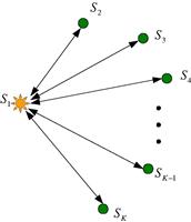
For this master-slave architecture, there exist two basic variations, depending on how the master element interacts with each of these slave elements. The first one is the open-loop approach, in which the master node broadcasts an unmodulated sinusoidal reference signal to all the slave nodes, and each of these slave nodes will then use such a reference signal to estimate and correct its phase offset. In this way, interaction between the master node and slave nodes is minimal. However, the absence of a common time reference, as we pointed out earlier, makes it difficult for each sensor to generate absolute phase with respect to the true time. As a result, phase shift induced by the channel between the master node and each slave node can not be disambiguated at each slave node, and hence cannot be compensated either. So, this open-loop method may lead to inferior accuracy in phase synchronization. On the other hand, suppose the channel phase information can be measured in a certain way and then fed back explicitly to each slave node for appropriate phase compensation, the accuracy of phase synchronization can be much improved. This is the basic idea behind the closed-loop approach, another type of master-slave synchronization. However, note that a fundamental premise that lies underneath this approach is the channel reciprocity, which is assumed in this work, meaning that the channel between a pair of sensors remains the same for both forward and reverse directions.
In the following, we describe a specific time-slotted closed-loop phase synchronization algorithm. In particular, we assume each slave element is assigned a specific time slot, during which they can exchange information with the master element ![]() . We further assume each slave element knows the number (or order) of the time slot assigned to it. This time-slotted closed-loop approach is then summarized as follows:
. We further assume each slave element knows the number (or order) of the time slot assigned to it. This time-slotted closed-loop approach is then summarized as follows:
1. ![]() broadcasts an unmodulated beacon signal to all the slave elements.
broadcasts an unmodulated beacon signal to all the slave elements.
2. Upon receiving the beacon signal, each slave sensor performs the following steps concurrently:
a. It estimates the frequency and phase of the received signal.
b. It begins to count the elapsed time using its own local clock, and waits for its time slot to come.
3. When the time slot for slave element ![]() starts according to its local clock, the following steps will take place in a sequential order:
starts according to its local clock, the following steps will take place in a sequential order:
a. ![]() passes the received beacon signal back to
passes the received beacon signal back to ![]() , using the local phase and frequency estimates generated from its observation.
, using the local phase and frequency estimates generated from its observation.
b. Upon receiving the returned beacon signal from ![]() ,
, ![]() estimates the received phase, and computes the phase difference relative to the originally transmitted reference signal. It divides the phase difference by two, pre-compensates the phase offset, and then transmits the beacon signal back to
estimates the received phase, and computes the phase difference relative to the originally transmitted reference signal. It divides the phase difference by two, pre-compensates the phase offset, and then transmits the beacon signal back to ![]() .
.
c. After receiving the reference signal, ![]() estimates the phase information and adjusts its carrier phase accordingly.
estimates the phase information and adjusts its carrier phase accordingly.
As is evident from the above procedures, it is essential to estimate the pre-compensation phase offset for each slave node when performing this closed-loop phase synchronization scheme. But since the channel between the master node and each slave node may vary from time to time, though at a slow rate, the value of the pre-compensation offset has to be estimated and updated in a periodic manner. A detailed timing analysis and phase synchronization error analysis of this algorithm can be found in [45].
2.13.6.2 Round-trip phase synchronization
The round-trip phase synchronization algorithm, as detailed in [45], was inspired by the all-node-based method proposed in [41] to globally synchronize the clocks in a sensor network, and the time-slotted round-trip approach that was developed in [42] and further improved or modified in [43,44] to attain carrier synchronization for distributed beamforming in multiuser wireless communication systems. The above mentioned approaches, nevertheless, do not appear to be applicable to this MIMO radar phase synchronization problem directly, even though a common feature shared by these approaches, that when in operation, a reference signal or message traverses in loops through all the sensors, remains essential.
The round-trip phase synchronization scheme for coherent MIMO radar [45] employs an unmodulated beacon signal to travel through all these radar elements in a round-trip manner. Each node will record the phase information twice in order to compute the final phase. The equivalence of the cumulative phase shift at each sensor, a quantity that is directly related to the total propagation delay for the round-trip circuit, is the fundamental idea behind this technique. This technique employs pretty much the same assumptions as those in the master-slave closed-loop method. For example, this scheme also assumes no a priori establishment of both time and frequency synchronization across all the radar elements, and assumes the channel reciprocity. However, specific to this round-trip method, we further assume that when one sensor transmits, the signal is only properly received by its intended receiver, i.e., its downstream neighbor. This can be attained in practice, for example, by using directional transmissions or appropriate power control schemes at the transmitter (assuming each radar element loosely knows its and its immediate neighbors’ locations). In what follows, we summarize this round-trip phase synchronization algorithm. Its mathematical characterization, timing analysis, and error analysis can be found in [45]:
1. Find a cycle which passes through all the radar elements. The radar elements are then labeled in order as ![]() . Let
. Let ![]() be the initiating element.
be the initiating element.
2. In time slot ![]() , an unmodulated sinusoidal reference signal is transmitted from
, an unmodulated sinusoidal reference signal is transmitted from ![]() to its downstream neighbor
to its downstream neighbor ![]() . This reference signal is further passed along the cycle in a clockwise manner, as illustrated by solid lines in Figure 13.13.
. This reference signal is further passed along the cycle in a clockwise manner, as illustrated by solid lines in Figure 13.13.
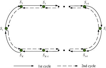
3. Upon receiving the reference signal, each radar element ![]() generates its local phase and frequency estimates from the noisy observation. In time slot
generates its local phase and frequency estimates from the noisy observation. In time slot ![]() , which starts immediately after the conclusion of the received signal,
, which starts immediately after the conclusion of the received signal, ![]() relays the received reference signal to the next node in the cycle.
relays the received reference signal to the next node in the cycle. ![]() will be the downstream neighbor of
will be the downstream neighbor of ![]() .
.
4. After the initiating node ![]() receives the signal from
receives the signal from ![]() , it generates a phase estimate from its noisy observation. Time slot
, it generates a phase estimate from its noisy observation. Time slot ![]() starts right after the conclusion of the received signal, wherein
starts right after the conclusion of the received signal, wherein ![]() transmits the original unmodulated sinusoidal reference signal as in step (1) to sensor
transmits the original unmodulated sinusoidal reference signal as in step (1) to sensor ![]() . This signal is passed along the cycle in the counterclockwise direction, as shown by dashed lines in Figure 13.13.
. This signal is passed along the cycle in the counterclockwise direction, as shown by dashed lines in Figure 13.13.
5. Upon receiving the signal transmitted from its upstream neighbor, each sensor ![]() generates its local phase and frequency estimates from its observation, and calculates its final phase based on its two-time phase estimates. In time slot
generates its local phase and frequency estimates from its observation, and calculates its final phase based on its two-time phase estimates. In time slot ![]() ,
, ![]() relays the received signal to the next node in the cycle, i.e.,
relays the received signal to the next node in the cycle, i.e., ![]() .
.
6. Relay of the beacon signal ends after ![]() finishes its receipt of the signal from
finishes its receipt of the signal from ![]() .
. ![]() generates a phase estimate from its noisy observation, and then calculates its final phase.
generates a phase estimate from its noisy observation, and then calculates its final phase.
2.13.6.3 Broadcast consensus based phase synchronization
It can be easily seen that the aforedescribed master-slave closed-loop and round-trip phase synchronization algorithms are not distributed in nature. Thus, both methods are not very robust against node failures. As far as robustness and scalability is concerned, distributed algorithms have enormous advantages, and may be more desirable for phase synchronization in coherent MIMO radar systems. The essence of these algorithms is that one or more sensors can communicate information with its immediate neighbors in a round, and the computation is distributed over all the sensors involved. In particular, when information averaging is concerned, these distributed algorithms are usually referred to as distributed consensus algorithms or gossip algorithms, e.g., [46–54]. Distributed consensus algorithms have been applied to a variety of network-related scenarios. For example, they have been considered in [53,54] for clock or time synchronization in wireless sensor networks.
Among the various distributed consensus algorithms, of particular note is the broadcast-based consensus algorithm, which has been studied in [50,51] without considering the stochastic disturbances, and more recently in [52] by taking non-zero-mean stochastic perturbations into account. Here we describe a broadcast consensus based phase synchronization algorithm for coherent MIMO radar systems, which was developed in [45], and is a direct extension of the work given in [52]. Similar to the aforedescribed two phase synchronization approaches, this algorithm assumes no a priori time synchronization; thus, there is no common time scale established among all these sensors. Each radar element is assumed to operate according to its own local clock which ticks independently from others. Also, for the ease of exposition, we assume the carrier frequency synchronization is already established, while noting that this assumption can be also relaxed. Thus, when a sensor receives beacon signals from its neighbors, it only needs to estimate the received phase.
In this algorithm, each element broadcasts a reference signal containing its local phase information to all its immediate neighbors. Its neighbors then average their local phase with the received phase. Thus, no global operations or information exchanges are required in the process. As an inherent characteristic, this algorithm exploits the broadcast nature of the wireless communication environment, and obviates the need for sophisticated underlying media access control mechanisms. To this end, we briefly outline this phase synchronization algorithm. Its mathematical characterization and analysis is furnished in [45], which examines in detail how the propagation delays among neighboring sensors and the phase errors induced by inaccurate local estimation affect the phase synchronization accuracy:
1. Sensor ![]() elects to broadcast an unmodulated reference signal.
elects to broadcast an unmodulated reference signal.
2. Each neighbor of ![]() , upon receiving the broadcast reference signal, generates an estimate of the received phase. If it is the first time for
, upon receiving the broadcast reference signal, generates an estimate of the received phase. If it is the first time for ![]() to receive a broadcast reference signal, it updates its phase with a weighted value of the phase estimate; otherwise, it updates its phase with a weighted average of its current phase and the phase estimate.
to receive a broadcast reference signal, it updates its phase with a weighted value of the phase estimate; otherwise, it updates its phase with a weighted average of its current phase and the phase estimate.
3. The phase of each of the remaining sensors, including ![]() , remains unchanged.
, remains unchanged.
4. This procedure continues, with each radar element having the same probability to broadcast in every round.
Note that the absence of a common time reference implies that none of these sensors know the true time, and as a result, they do not know the “true” initial phase of their local oscillator. Thus, when a sensor receives a broadcast reference signal for the first time, we choose to update its phase using only the estimate of the received phase.
2.13.6.4 Discussion
As can be clearly seen, the master-slave closed-loop method is the simplest one among all these three approaches. It, however, has the potential to lead to the best phase synchronization accuracy. This is because there are only two (the least number) nodes which participate in each round of the phase synchronization process, i.e., the master node and one slave node. Thus, the propagating accumulation of each individual’s phase and frequency estimation errors is very limited, and is less of a concern. This, in fact, is corroborated by a rigorous phase synchronization error analysis included in [45]. Moreover, in this method, the phase offset induced by the propagation channel is explicitly compensated via the closed-loop operation, which further improves the phase synchronization accuracy. Therefore, this approach is particularly useful when a very precise phase synchronization is required. It is generally applicable to situations where a relatively powerful centralized entity exists or can be identified, and can be repeatedly used in systems having tree-like topologies or hierarchical structures. To complete the whole phase synchronization process, a total of ![]() transmissions are needed, including the broadcast transmission made by the master node.
transmissions are needed, including the broadcast transmission made by the master node.
Unlike the master-slave closed-loop method, both the round-trip and the broadcast consensus based algorithms do not require a powerful master entity. However, the round-trip scheme does need a global initiator to start the phase synchronization process. In theory, the global initiator can be any radar sensor in the system. This round-trip method is able to synchronize all the radar sensors to the same mean carrier phase, regardless of the topology of these sensors as long as a cycle traversing all these sensors can be identified. But since sensors in the system participate in the phase synchronization process all together in a cooperative fashion, this round-trip method may suffer from the propagating accumulation of each individual’s phase and frequency estimation errors, as mathematically demonstrated in [45]. As a result, this method may only be suitable to coherent MIMO radar systems with a limited number of sensors. In other words, it does not scale very well. This round-trip method needs a total of ![]() transmissions to complete the phase synchronization process.
transmissions to complete the phase synchronization process.
The broadcast consensus based method is distributed and localized in nature. It needs neither a centralized entity nor a particular global initiator. It is scalable and applicable to coherent MIMO radar systems composed of a large number of densely scattered sensors. It is also robust to sensor failures. But unfortunately, as shown in [45], the functionality of this approach is highly dependent on, and varies from topology to topology of the radar sensors. For arbitrary topologies, this approach may be only useful when a coarse phase synchronization is required. Since this algorithm runs in an iterative manner, it generally requires more transmissions than the other two approaches to complete the whole synchronization process. Thus, it has to be implemented at a relaxed time constraint as opposed to a stringent one.
Of further note is that in each of the presented phase synchronization algorithms, the propagation delay for the channel between any pair of MIMO radar elements that are involved in the reference signal exchange, can be critical in determining the resulting phase synchronization accuracy. A small uncertainty in the channel propagation delay, which may result from, for example, the ambiguity in the location of certain radar elements or the mobile scatters and other propagation anomalies, can lead to intolerable phase variations across some or all the radar elements. This is particularly true when high frequency carriers are chosen as the reference signals. One way to alleviate this unfavorable effect is to use relatively low carrier frequency. If the carrier frequency is low enough, the location uncertainty of the MIMO radar elements will not play an important role. Another way is to recalibrate these sensors periodically to track the channel changes. This may induce some extra overhead, but the accompanying benefits are in general well worth it. Besides, the variations of the propagation channels among all these MIMO radar elements, though dependent on the specific operating environment, are usually very slow; it takes a relatively long time to reach the point where the physical changes in the medium are so pronounced that the resulting phase mismatch seriously deteriorates the performance of the coherent processing, especially for applications such as target localization [11]. Therefore, very frequent phase resynchronization may not be needed.
Another practical issue that merits attention is the phase dynamics or phase instability [55] in the coherent MIMO radar system. Note that the oscillator phase noise [56] is always present, and is an irreducible error which can affect the phase synchronization performance. To counter the effect of phase noise in oscillators, periodic phase synchronization remains indispensable. How often the phase synchronization procedure needs to be repeated, however, is dependent on, among other factors, the aggregate impact of the phase noise across all the local oscillators on the phase synchronization accuracy, as well as the phase accuracy or stability requirements of the coherent MIMO radar system and the specific application. It is indicated in [34, p. 261] that the phase accuracy or stability requirements for coherent processing by a monostatic or bistatic radar can range from less than one degree to many tens of degrees of RF phase over a coherent processing interval, depending on the type and duration of coherent processing. We conjecture that similar phase accuracy or stability requirements may hold as well for coherent processing by a MIMO radar system.
2.13.7 Waveform design for MIMO radar
Most radar systems operate by radiating a specific electromagnetic signal into a region and detecting the echo returned from the reflecting targets. The nature of the echo signal provides information about the target, such as range, radial velocity, angular direction, size, shape and so on [57]. This signal is usually referred to as the radar waveform, and plays a key role in the accuracy, resolution, and ambiguity for radar in performing the above mentioned tasks [58]. For MIMO radar, it also relies on waveforms to realize its excellent performance advantages. Thus, the design of appropriate waveforms for MIMO radar has become a crucial task, which has attracted a lot of attention over the years. Recent work on waveform design for MIMO radar (with both widely separated antennas and colocated antennas) includes, among others, [9,12,59–74].
In this section, we will briefly describe a specific waveform design scheme for MIMO radar with widely separated antennas. This scheme was originally developed by us in [9], and further improved or extended later in, for example [59,60]. It is primarily focused on optimizing MIMO radar’s performance in information extraction and estimation of extended targets which are modeled using an impulse response as in [75] (point targets are a special case). Assuming that the radar transmitter has some knowledge (full or partial) of the target’s second-order statistics and that the transmitted power is constrained, Yang and Blum [9] detail methods for finding waveform design strategies based on the following two criteria: (1) maximizing the conditional mutual information (MI) between the random target impulse response and the reflected radar waveforms; (2) minimizing the value of minimum mean-square error (MMSE) in estimating the target impulse response. In this part, we will concisely summarize some major results of [9], and shed some light on the waveform design problem for MIMO radar.
2.13.7.1 Signal model and design criteria
Figure 13.14 illustrates a bistatic MIMO radar scenario, where the radar is equipped with ![]() transmit elements and
transmit elements and ![]() receive elements. This model, appropriate for both bistatic and monostatic scenarios, is a slight generalization of that in [2] for the case of extended targets. For simplicity we consider this model in discrete-time and in baseband. For an extended target, the reflection from the signal sent from the
receive elements. This model, appropriate for both bistatic and monostatic scenarios, is a slight generalization of that in [2] for the case of extended targets. For simplicity we consider this model in discrete-time and in baseband. For an extended target, the reflection from the signal sent from the ![]() th transmit element and captured at the
th transmit element and captured at the ![]() th receive element can be modeled using a finite impulse response (FIR) linear system with order
th receive element can be modeled using a finite impulse response (FIR) linear system with order ![]() , whose impulse response is
, whose impulse response is ![]() . Then the received waveform at the
. Then the received waveform at the ![]() th receive element and discrete-time
th receive element and discrete-time ![]() is given by
is given by
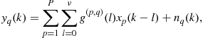 (13.97)
where ![]() is the waveform transmitted from the
is the waveform transmitted from the ![]() th transmit element and
th transmit element and ![]() is the additive complex Gaussian noise measured at the
is the additive complex Gaussian noise measured at the ![]() th receive element.
th receive element.
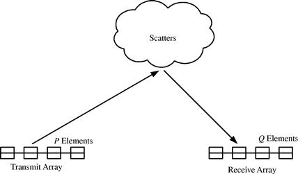
Let ![]() denote the length of the observed signal vector starting at an arbitrary discrete time
denote the length of the observed signal vector starting at an arbitrary discrete time ![]() , and assume that
, and assume that ![]() (typically
(typically ![]() ). Denote
). Denote ![]() and
and ![]() , then using the matrix-vector notation (13.97) can be rewritten into
, then using the matrix-vector notation (13.97) can be rewritten into
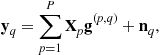 (13.98)
where ![]() is an
is an ![]() Toeplitz matrix which contains the waveforms transmitted from the
Toeplitz matrix which contains the waveforms transmitted from the ![]() th transmit element, i.e.,
th transmit element, i.e.,
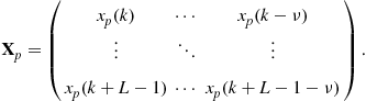 (13.99)
We further define ![]() and
and ![]() , so that (13.98) could be reformulated into
, so that (13.98) could be reformulated into
![]() (13.100)
(13.100)
By stacking the received waveforms across all the ![]() receive elements, we create
receive elements, we create ![]() . Defining
. Defining ![]() , we finally obtain
, we finally obtain
![]() (13.101)
(13.101)
where ![]() and
and ![]() .
.
To facilitate the ensuing analysis on the waveform design of MIMO radar for extended targets, the model in (13.101) is assumed to have the following properties [9]:
Assumption 4
The target impulse response vector![]() is a Gaussian random vector with zero mean and full rank covariance matrix
is a Gaussian random vector with zero mean and full rank covariance matrix![]() .
.
Assumption 5
Components of the noise vector![]() are assumed to be independently and identically distributed (i.i.d) and complex Gaussian, with zero mean and variance
are assumed to be independently and identically distributed (i.i.d) and complex Gaussian, with zero mean and variance![]() .
.
Note that ![]() can be diagonalized through its eigenvalue decomposition, i.e.,
can be diagonalized through its eigenvalue decomposition, i.e.,
![]() (13.102)
(13.102)
where ![]() is a unitary matrix whose columns are eigenvectors and
is a unitary matrix whose columns are eigenvectors and ![]() is a diagonal matrix with each diagonal entry given by a real and nonnegative eigenvalue.
is a diagonal matrix with each diagonal entry given by a real and nonnegative eigenvalue.
Now let us introduce the design criteria. The first one is the conditional mutual information (MI) between ![]() and
and ![]() given the knowledge of
given the knowledge of ![]() , which is hereafter referred to as MI. We have [76] (
, which is hereafter referred to as MI. We have [76] (![]() denotes differential entropy)
denotes differential entropy)
![]() (13.103)
(13.103)
Conditioned on ![]() (equivalent to conditioning on
(equivalent to conditioning on ![]() ), we can easily find that
), we can easily find that ![]() is Gaussian distributed with zero mean and covariance
is Gaussian distributed with zero mean and covariance ![]() . Using (13.103), the MI is [76]
. Using (13.103), the MI is [76]
 (13.104)
where (13.104) follows from
![]() (13.105)
(13.105)
The design objective is to find those ![]() (transmitted waveform) that maximize the MI (
(transmitted waveform) that maximize the MI (![]() ) between the random target impulse response
) between the random target impulse response ![]() and the received (reflected) radar waveform
and the received (reflected) radar waveform ![]() under the constraint
under the constraint ![]() which effectively limits the total transmit power. Therefore, the problem of waveform design based on MI can be cast as:
which effectively limits the total transmit power. Therefore, the problem of waveform design based on MI can be cast as:
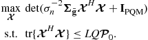
Next, let us consider the problem of radar waveform design from the viewpoint of estimation. It is easy to verify that, conditioned on ![]() ,
, ![]() , and
, and ![]() are jointly Gaussian distributed as
are jointly Gaussian distributed as

The conditional distribution of ![]() given
given ![]() and
and ![]() is also Gaussian, with conditional mean
is also Gaussian, with conditional mean ![]() given by (using Eqs. (IV.B.53) and (IV.B.55) on p. 156 of [17])
given by (using Eqs. (IV.B.53) and (IV.B.55) on p. 156 of [17])
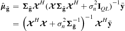 (13.106)
and conditional covariance matrix ![]() given by (using Eq. (IV.B.54) on pp. 156 of [17])
given by (using Eq. (IV.B.54) on pp. 156 of [17])
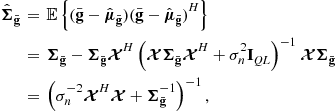 (13.107)
where the matrix inversion lemma11 was employed in obtaining both (13.106) and (13.107).
Let ![]() denote the Bayes estimate of
denote the Bayes estimate of ![]() . When the cost function is defined as
. When the cost function is defined as ![]() , the Bayes estimate
, the Bayes estimate ![]() will be a linear MMSE estimator [17] which is given by the conditional mean of
will be a linear MMSE estimator [17] which is given by the conditional mean of ![]() given
given ![]() (for a given value of
(for a given value of ![]() ), i.e.,
), i.e.,
![]() (13.108)
(13.108)
In this case, the Bayes risk for a given ![]() will be
will be
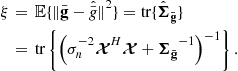 (13.109)
The goal is then to find those ![]() that minimize the value of MMSE under a constraint on the total transmit power of
that minimize the value of MMSE under a constraint on the total transmit power of ![]() . Or equivalently, the problem of waveform design based on MMSE estimation can be expressed as:
. Or equivalently, the problem of waveform design based on MMSE estimation can be expressed as:
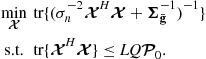
2.13.7.2 Optimal waveform design for MIMO radar
As mathematically demonstrated in [9], the maximum value of ![]() will be achieved when the matrix
will be achieved when the matrix ![]() is diagonal, and the minimum value of
is diagonal, and the minimum value of ![]() will be attained when
will be attained when ![]() is diagonal, also. The following theorem summarizes the result of optimum
is diagonal, also. The following theorem summarizes the result of optimum ![]() . A detailed proof of this result can be found in [9].
. A detailed proof of this result can be found in [9].
Theorem 3
Let Assumptions 4 and 5 hold true. Then![]() under the constraint
under the constraint![]() only
only![]() that satisfy
that satisfy
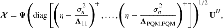 (13.110)
can be optimum in the sense of either maximizing the MI or minimizing the MMSE. In (13.110),![]() and
and![]() are defined in (13.102);
are defined in (13.102);![]() is an
is an![]() matrix with orthonormal columns
matrix with orthonormal columns![]() the scalar constant
the scalar constant![]() is chosen to satisfy
is chosen to satisfy

The resulting maximum value of MI is

and the corresponding minimum value of MMSE is
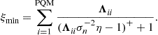
Further![]() provided
provided![]() for some
for some![]() then any
then any![]() satisfying (13.110)is optimum for both the MI and MMSE criteria.
satisfying (13.110)is optimum for both the MI and MMSE criteria.
A review of Theorem 3 indicates that knowledge of the full matrix ![]() is needed to perform an eigenvalue decomposition. An asymptotic formulation has been developed in [9] which lessens the required information to just a few samples of the PSD and would be much more suitable in practice. The asymptotic approach employs one important assumption as shown below:
is needed to perform an eigenvalue decomposition. An asymptotic formulation has been developed in [9] which lessens the required information to just a few samples of the PSD and would be much more suitable in practice. The asymptotic approach employs one important assumption as shown below:
Assumption 6
The covariance matrix![]() of
of![]() has a Toeplitz structure.
has a Toeplitz structure.
Clearly this assumption is not very restrictive for single transmit and receive antenna cases, implying that the target impulse response samples form a wide-sense stationary random process asymptotically. For multiple transmit and receive antenna cases, this assumption implies that the statistics over space are indistinguishable from the statistics over time. For the extreme cases of complete independence or dependence over both space and time, the assumption is very reasonable, for example. However, it is also straightforward to relax this assumption for multiple-antenna cases by employing a similar asymptotic approximation as that described below. For a further discussion on this assumption, readers are referred to [59].
It is shown in [77] that Toeplitz matrices can be approximated by their associated circulant matrices, and asymptotically (in the dimension of these matrices), they are equivalent. The asymptotic equality of two matrices implies that their eigenvalues and inverses (and certain products) behave similarly [77]. Now, let us denote the ![]() th entry of the covariance matrix
th entry of the covariance matrix ![]() as
as ![]() , then we have
, then we have ![]() and
and ![]() , where the sequence
, where the sequence ![]() is absolutely summable, and its
is absolutely summable, and its ![]() -periodic truncated Fourier spectrum
-periodic truncated Fourier spectrum
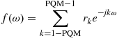
is real valued, finite, and nonnegative, and represents the PSD of the random process ![]() when
when ![]() approaches infinity. Then a circulant matrix
approaches infinity. Then a circulant matrix ![]() that is asymptotically equivalent to
that is asymptotically equivalent to ![]() is [78]
is [78]
![]() (13.111)
(13.111)
where ![]() is the
is the ![]() unitary discrete Fourier transform (DFT) matrix with its
unitary discrete Fourier transform (DFT) matrix with its ![]() th entry given by
th entry given by
![]()
and the diagonal matrix ![]() contains samples of the PSD of
contains samples of the PSD of ![]() along its diagonal, or equivalently
along its diagonal, or equivalently
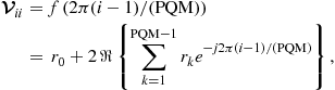
where ![]() .
.
Given the above asymptotic approximation, the waveform design problems posed earlier can be resolved using standard optimization theory. For brevity, we summarize the results in the following theorem. The proof can be found in [9].
Theorem 4
Suppose Assumptions 4–6 hold true and perfect knowledge is available on the samples of the target PSD![]() i.e.
i.e.![]() entries in the diagonal matrix
entries in the diagonal matrix![]() . Then under a constraint
. Then under a constraint![]() only a signaling matrix
only a signaling matrix![]() that satisfies
that satisfies
![]() (13.112)
(13.112)
can be asymptotically optimum in the sense of either maximizing the MI or minimizing the MMSE![]() where we have
where we have
 (13.113)
and the constant![]() is chosen to satisfy
is chosen to satisfy
 (13.114)
Further, any![]() from (13.112)is asymptotically optimum for both MI and MMSE.
from (13.112)is asymptotically optimum for both MI and MMSE.
In fact, Theorem 4 is simply a modification of Theorem 3 for the asymptotic case. The essential change is that ![]() replaces
replaces ![]() and
and ![]() replaces
replaces ![]() . Under such asymptotic approximation, the solution for
. Under such asymptotic approximation, the solution for ![]() can be explicitly written as
can be explicitly written as
 (13.115)
It is obvious that to produce ![]() in (13.115), the full covariance matrix
in (13.115), the full covariance matrix ![]() is not needed, only samples of the PSD for
is not needed, only samples of the PSD for ![]() are necessary. This is a more reasonable assumption in practice.
are necessary. This is a more reasonable assumption in practice.
2.13.7.3 Discussion
Based on Theorem 3, it can be concluded that any ![]() meeting the given power constraint which maximizes MI will also minimize MMSE, and this
meeting the given power constraint which maximizes MI will also minimize MMSE, and this ![]() is unique for a given
is unique for a given ![]() . In fact,
. In fact, ![]() can be deemed as the covariance matrix of the transmitted waveforms. Meanwhile, it should be noted that the solution expressed by (13.110) is a closed-form and general solution which does not require any level of approximation. Its optimality is manifested in two ways. On the one hand, only
can be deemed as the covariance matrix of the transmitted waveforms. Meanwhile, it should be noted that the solution expressed by (13.110) is a closed-form and general solution which does not require any level of approximation. Its optimality is manifested in two ways. On the one hand, only ![]() satisfying (13.110) can be optimum in the sense of either maximizing the MI or minimizing the MMSE. On the other hand, any
satisfying (13.110) can be optimum in the sense of either maximizing the MI or minimizing the MMSE. On the other hand, any ![]() from (13.110) is optimum for both MI and MMSE provided such
from (13.110) is optimum for both MI and MMSE provided such ![]() satisfies
satisfies ![]() . In other words, the condition stipulated by (13.110) is only a necessary condition for
. In other words, the condition stipulated by (13.110) is only a necessary condition for ![]() to attain the optimality, but not a sufficient one. This is because there may exist some cases where a solution
to attain the optimality, but not a sufficient one. This is because there may exist some cases where a solution ![]() satisfies (13.110) but does not have the desired Kronecker structure. Note for these cases, it can be possible that the equivalence between the MI and the MMSE does not hold any more. However, in a recently published paper [60], an iterative algorithm has been developed, which can identify waveform solutions that not only optimize the performance criteria of interest (i.e., MI and MMSE), but have a specific Kronecker structure. It is also found in [60] that waveform solutions generated through this algorithm can lead to performance which is very close to, and almost indistinguishable from that predicted by Theorem 3. Detailed information about this algorithm can be found in [60].
satisfies (13.110) but does not have the desired Kronecker structure. Note for these cases, it can be possible that the equivalence between the MI and the MMSE does not hold any more. However, in a recently published paper [60], an iterative algorithm has been developed, which can identify waveform solutions that not only optimize the performance criteria of interest (i.e., MI and MMSE), but have a specific Kronecker structure. It is also found in [60] that waveform solutions generated through this algorithm can lead to performance which is very close to, and almost indistinguishable from that predicted by Theorem 3. Detailed information about this algorithm can be found in [60].
A close review of Theorem 4 reveals that for the asymptotic simplification approach, exact knowledge of the target PSD samples is required in the waveform design. This requirement appears rather demanding, particulary in practical applications. In order to bring the waveform design even closer to practice and deliver more applicable waveform solutions for MIMO radar, it is necessary to accommodate some issues that may arise in reality, such as the uncertainty in the target’s statistics. In such a circumstance, robust procedures, which can overcome those problems by incorporating modeling uncertainty into the design from the outset [79], seem quite attractive. As a result, a minimax robust waveform design problem for MIMO radar has been formulated and solved in [59], where a band model was adopted by assuming the PSD lies in an uncertainty class of spectra bounded by known upper and lower bounds. This band model might arise in practice, for example, if a confidence band for the spectrum could be determined via spectrum estimation, or the upper and lower bounds can be obtained simply by field measurement and modeling. It is shown in [59] that the resulting minimax robust waveforms can achieve good performance for any PSD in the uncertainty class, and in particular, they can bound the worst-case performance at an acceptable limit. One very interesting finding from the results in [59] is that the minimax robust waveforms for the MMSE criterion are generally different from those for the MI criterion, which is in stark contrast to the results for the completely known PSD case. We direct interested readers to [59] for more details.
2.13.8 Summary
In this document, we provided a review of some key topics related to MIMO radar with widely separated antennas. This type of MIMO radar features two major configurations, one with all antennas within a same target beamwidth and one with antennas placed in distinct target beamwidths, which, in turn, lead to two different operation modes called coherent and noncoherent MIMO radars, respectively. In Sections 2.13.2 and 2.13.3, signal models for coherent and noncoherent MIMO radars were introduced for the problem of joint target location and velocity estimation. Equations specifying the ML estimates were derived for some general cases, which accommodate scenarios featuring, for example, nonorthogonal transmitted waveforms, spatially colored clutter-plus-noise, and correlated reflection coefficients. However, to provide further insight, we also considered some simplified cases, where orthogonal waveforms, temporally and spatially white clutter-plus-noise, and independent reflections are assumed. The MSEs of the ML estimates, the corresponding CRBs, and the coherent and noncoherent AFs were presented.
In Section 2.13.4, the performance and complexity issues for the coherent and noncoherent MIMO radars were investigated. Although the coherent MIMO radar outperforms the noncoherent one in general, it has more stringent operational requirement and incurs more implementation complexity. Fortunately, our results indicate that for some cases, e.g., when ![]() is sufficiently large, we can replace the coherent approach by its noncoherent counterpart, which, while reducing a great deal the implementation complexity, induces very little loss of performance. As a result, if large
is sufficiently large, we can replace the coherent approach by its noncoherent counterpart, which, while reducing a great deal the implementation complexity, induces very little loss of performance. As a result, if large ![]() can be afforded in practice, the noncoherent MIMO radar is naturally preferred to the coherent one. The NDRMSE was defined in this section, and was used to compare the overall performance difference between the coherent and noncoherent MIMO radars for joint parameter estimation. A sufficiently small value of the parameter NDRMSE can serve as an indicator, suggesting the noncoherent MIMO radar performs very well relative to the coherent one.
can be afforded in practice, the noncoherent MIMO radar is naturally preferred to the coherent one. The NDRMSE was defined in this section, and was used to compare the overall performance difference between the coherent and noncoherent MIMO radars for joint parameter estimation. A sufficiently small value of the parameter NDRMSE can serve as an indicator, suggesting the noncoherent MIMO radar performs very well relative to the coherent one.
The diversity gains were analyzed for MIMO radar target detection under the Neyman-Pearson criterion in Section 2.13.5. We showed that the maximum achievable diversity gain for a MIMO radar system is determined by the number of transmit antennas, the number of scatterers that compose the target, the dimension spanned by the clutter-plus-noise free received waveforms at each receiver, and the cdf of the reflection coefficients, while it is invariant to the clutter-plus-noise cdf, provided the magnitude of the processed clutter-plus-noise has bounded moments up to a required order. It was shown that for some cases of interest, the maximum diversity gain can be achieved. Further, properly chosen nonorthogonal waveforms can achieve the same diversity gain as orthogonal waveforms.
In Section 2.13.6, we discussed three effective approaches to achieve phase synchronization in coherent MIMO radar systems. The first one is the master-slave closed-loop approach, which employs a master-slave architecture. This method is very simple, and is suitable for fine phase synchronization. The second one is the round-trip algorithm, which employs an unmodulated beacon signal to travel through all the radar elements in a round-trip manner. This method is applicable to arbitrary topologies of the radar sensors as long as a cycle traversing all these sensors can be identified. The third one is the broadcast consensus based algorithm, which is scalable, and is distributed and localized in nature. Distinct as they are, these algorithms are all time asynchronous, and in particular, the master-slave closed-loop algorithm and the round-trip algorithm also require no a priori frequency synchronization. These algorithms should cater to different needs arising as a result of different number of MIMO radar elements, different sensor placements, as well as different operational preferences.
Several MIMO radar waveform design methods were presented in Section 2.13.7. The discussed methods capitalize on the knowledge of the covariance matrix of the extended target impulse response, and optimize two criteria: maximization of the MI and minimization of the MMSE. For both design criteria, a constraint on the transmitted power is imposed. The findings indicate that these two criteria are equivalent in the sense that they lead to the same covariance matrix of the transmit waveforms, which is a fundamental quantity specifying the waveform design. The optimum solution employs water-filling, which allocates the transmitted power in proportion to the quality of the particular mode in question. In particular, more transmitted waveform power is allocated to modes that have higher power, indicating the presence of significant target scattering, and modes with low power deserve excitation with lower transmitted waveform power. In addition, an asymptotic formulation was also provided in Section 2.13.7, which lessens the required knowledge about the target statistical model to just a few samples of the PSD, and would be much more suitable in practice.
Notation
Throughout this chapter, we use bold upper case letters to denote matrices, and bold lower case letters to signify column vectors. The definition of symbols used in this chapter are listed below:
![]() expectation with respect to all the random variables within the brackets
expectation with respect to all the random variables within the brackets
![]() conjugate transpose of the argument
conjugate transpose of the argument
![]() absolute value of a complex number
absolute value of a complex number
![]() Euclidean norm of the argument
Euclidean norm of the argument
![]() imaginary part of a complex number
imaginary part of a complex number
![]() little-o notation, i.e., Suppose
little-o notation, i.e., Suppose ![]() and
and ![]() are both functions of a variable
are both functions of a variable ![]() , then
, then ![]() as
as ![]() implies
implies ![]()
![]()
![]() unit impulse function, i.e.,
unit impulse function, i.e., ![]() if
if ![]() or
or ![]() if
if ![]()
![]() diagonal matrix with elements
diagonal matrix with elements ![]() on its diagonal
on its diagonal
![]() block diagonal matrix with submatrices
block diagonal matrix with submatrices ![]() on its diagonal
on its diagonal
Appendix
A.1 Frequency spread signals
In this appendix, we describe one class of signals which could be employed. Under appropriate assumptions, these signals approximately satisfy the conditions of Assumption 1 for orthogonal signals. We discuss these assumptions. These assumptions essentially ignore small sidelobes in the Fourier transform of these signals to approximate them with truncated (in frequency domain) signals.
Consider a set of pulsed sinusoidal signals12
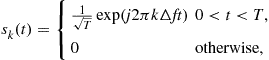 (A.1)
(A.1)
where ![]() , the term
, the term ![]() denotes the signal time duration, and
denotes the signal time duration, and ![]() is the frequency increment between
is the frequency increment between ![]() and
and ![]() . The approximate bandwidth of each signal is
. The approximate bandwidth of each signal is ![]() . The spectrum of
. The spectrum of ![]() and
and ![]() and
and ![]() , are shown in Figure A.1. Note that throughout this appendix it is always assumed that
, are shown in Figure A.1. Note that throughout this appendix it is always assumed that ![]() . According to Parseval’s theorem
. According to Parseval’s theorem
![]() (A.2)
(A.2)
Observing the spectrum, we see that when ![]() , the main lobes of
, the main lobes of ![]() and
and ![]() are sufficiently separated so that
are sufficiently separated so that ![]() and (A.2) approximates
and (A.2) approximates ![]() , which makes
, which makes ![]() and
and ![]() approximately orthogonal. Here we are ignoring contributions from small sidelobes which is similar to truncating the signals in the frequency domain. As
approximately orthogonal. Here we are ignoring contributions from small sidelobes which is similar to truncating the signals in the frequency domain. As ![]() , if the frequency increment satisfies
, if the frequency increment satisfies
![]() (A.3)
(A.3)
then any two signals from the signal set ![]() (
(![]() ) are approximately orthogonal.
) are approximately orthogonal.
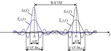
Figure A.1 Frequency spectrum for transmitted signals (solid curves) and the effective parts of their time delayed versions (dotted curves).
Assume that ![]() and
and ![]() are time delayed by
are time delayed by ![]() and
and ![]() . The non-zero part of the delayed signal
. The non-zero part of the delayed signal ![]() occupies
occupies ![]() , and the non-zero part of
, and the non-zero part of ![]() occupies
occupies ![]() . Hence, the time duration of the overlap between them is
. Hence, the time duration of the overlap between them is ![]() , where
, where ![]() denotes the time delay difference. Note that when
denotes the time delay difference. Note that when ![]() is greater than or approximates
is greater than or approximates ![]() , the overlap part of these two signals vanishes, which implies (A.2) is close to
, the overlap part of these two signals vanishes, which implies (A.2) is close to ![]() and the signals can be considered as orthogonal. Therefore, it is possible for the two delayed signals to be non-orthogonal only if
and the signals can be considered as orthogonal. Therefore, it is possible for the two delayed signals to be non-orthogonal only if ![]() , which makes the following discussion necessary.
, which makes the following discussion necessary.
We denote the overlap interval as ![]() . Thus
. Thus

where ![]() and
and ![]() represent the overlapping parts of
represent the overlapping parts of ![]() and
and ![]() , the time duration of which are both
, the time duration of which are both ![]() . More specifically, suppose
. More specifically, suppose ![]() , then we have
, then we have
![]()
The spectrum of ![]() and
and ![]() , i.e.,
, i.e., ![]() and
and ![]() , are plotted by dotted curves in Figure A.1. In a similar way, for the time delayed signals, the orthogonality is approximately maintained if
, are plotted by dotted curves in Figure A.1. In a similar way, for the time delayed signals, the orthogonality is approximately maintained if
![]() (A.4)
(A.4)
Since ![]() , the inequality is maintained by requiring
, the inequality is maintained by requiring ![]() . As
. As ![]() , the condition becomes
, the condition becomes ![]() , which is the same as in (A.3). Hence, the requirement for (A.3) guarantees (A.4). That is, if (A.3) is met, the time delayed signals are orthogonal.
, which is the same as in (A.3). Hence, the requirement for (A.3) guarantees (A.4). That is, if (A.3) is met, the time delayed signals are orthogonal.
Next, we further discuss the Doppler shift restriction for orthogonality. The effective time delayed and Doppler shifted signals are given by ![]() and
and ![]() . The frequency spectrum of the effective time delayed signals
. The frequency spectrum of the effective time delayed signals ![]() and
and ![]() , i.e.,
, i.e., ![]() and
and ![]() , are replotted in Figure A.2 using solid curves, the center frequency of which are
, are replotted in Figure A.2 using solid curves, the center frequency of which are ![]() and
and ![]() . After Doppler frequency shift, the spectrum of the effective time delayed and Doppler shifted signals are
. After Doppler frequency shift, the spectrum of the effective time delayed and Doppler shifted signals are ![]() and
and ![]() . They are shown in Figure A.2 using dashed curves. Thus, the center frequency of the effective signal
. They are shown in Figure A.2 using dashed curves. Thus, the center frequency of the effective signal ![]() is
is ![]() , while the center frequency of
, while the center frequency of ![]() becomes
becomes ![]() . Clearly, provided
. Clearly, provided ![]() , that is
, that is
 (A.5)
(A.5)
the overlapping part between ![]() and
and ![]() (
(![]() ) can be ignored. Thus the orthogonality is well approximated. Note that since (A.4) is satisfied, we have
) can be ignored. Thus the orthogonality is well approximated. Note that since (A.4) is satisfied, we have ![]() . Hence the term
. Hence the term ![]() in (A.5) can be ignored, resulting in
in (A.5) can be ignored, resulting in ![]() or
or ![]() .
.
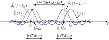
Figure A.2 Frequency spectrum for the time delayed equivalent signals (solid curves) and their Doppler shifted versions (dotted curves).
It has been shown in [24] that, in the example case of target velocity estimation, the CRBs obtained using untruncated signals under certain conditions that are of practical interest are extremely close to the CRBs calculate by assuming ideal orthogonal signals. Interested readers are referred to [24] for detail.
A.2 Distinguishing coherent and noncoherent processing
In the MIMO radar context, the term coherent processing implies that the relative phase information embedded in the signals traveling over the paths between different transmit and receive antennas will be exploited (e.g., see (13.22)). Ultimately, this requires the oscillators in the up and down converters at different transmit and receive antenna nodes to be locked in phase. This is not the case for noncoherent processing where the relative phase information is not exploited (e.g., see (13.57)).
To distinguish between the coherent and noncoherent processing, one can examine the output of the processor (e.g., (13.22) or (13.57)), say denoted by ![]() , as a function of a set of observations coming from different spatial paths, say denoted by
, as a function of a set of observations coming from different spatial paths, say denoted by ![]() , where
, where ![]() represents the number of available observations coming from different spatial paths. That is
represents the number of available observations coming from different spatial paths. That is ![]() . If an arbitrary constant13 phase set
. If an arbitrary constant13 phase set ![]() is imposed on the observations coming from different spatial paths, but the processing is insensitive to the phase shifts over the different paths, i.e., the output of the processor
is imposed on the observations coming from different spatial paths, but the processing is insensitive to the phase shifts over the different paths, i.e., the output of the processor ![]() is not affected, such that
is not affected, such that
![]() (A.6)
(A.6)
then the processor is regarded as being noncoherent. Otherwise, if the output of the processor is affected by the arbitrary phase set, such that
![]() (A.7)
(A.7)
then the processor is regarded as being coherent.
The estimators ![]() in (13.22) and
in (13.22) and ![]() in (13.57), which satisfy (A.7) and (A.6), are examples of noncoherent and coherent processors respectively, where
in (13.57), which satisfy (A.7) and (A.6), are examples of noncoherent and coherent processors respectively, where
![]()
and
![]()
A.3 FIM for coherent MIMO radar joint estimation
Considering that the log-likelihood ratio in (13.20) is explicitly a function of ![]() and
and ![]() , but implicitly as a function of
, but implicitly as a function of ![]() , we defined a new parameter vector
, we defined a new parameter vector
![]() (A.8)
(A.8)
Then, the FIM can be derived using the chain rule as
![]() (A.9)
(A.9)
We first compute ![]() and obtain
and obtain
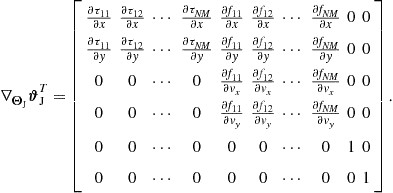
Partitioning ![]() into a block matrix, we have
into a block matrix, we have
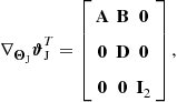
where ![]() are
are ![]() submatrices. The
submatrices. The ![]() in (A.9) can be derived from (13.20) as
in (A.9) can be derived from (13.20) as
![]()
which is a ![]() matrix. Write
matrix. Write ![]() in the form of a block matrix
in the form of a block matrix

where ![]() are
are ![]() matrices. Carrying out the computation, we get
matrices. Carrying out the computation, we get
![]() (A.10)
(A.10)
![]() (A.11)
(A.11)
![]() (A.12)
(A.12)
![]() (A.13)
(A.13)
![]() (A.14)
(A.14)
and
![]() (A.15)
(A.15)
where the terms ![]() ,
, ![]() ,
, ![]() dependent on the characteristics of the received waveforms are provided in (A.9)–(A.13). Thus, the FIM can be computed through
dependent on the characteristics of the received waveforms are provided in (A.9)–(A.13). Thus, the FIM can be computed through
 (A.16)
After lengthy algebraic manipulations, the expression of the FIM can be obtained as shown in (13.23).
A.4 Calculating FIM for localization with phase errors
First, let us compute the ![]() th (
th (![]() ) element of the matrix. Referring to the vector in (13.41), let
) element of the matrix. Referring to the vector in (13.41), let ![]() refer to the index of the element of
refer to the index of the element of ![]() corresponding to
corresponding to ![]() , then let
, then let ![]() refer to the index of the element of
refer to the index of the element of ![]() corresponding to
corresponding to ![]()
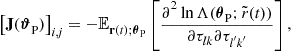 (A.17)
where
![]() (A.18)
(A.18)
The term ![]() in (A.18) is given in (13.39). Further
in (A.18) is given in (13.39). Further
![]() (A.19)
(A.19)
where ![]() is given in (13.38). Assuming an interchange of derivative and integral is valid,14 then
is given in (13.38). Assuming an interchange of derivative and integral is valid,14 then
 (A.20)
 (A.21)
Finally, the remaining term in (A.18) is
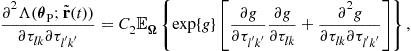
where for ![]() , and for
, and for ![]()
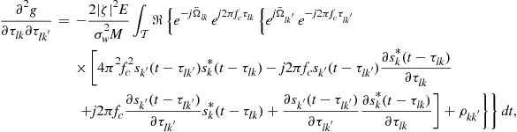
where for ![]() , and for
, and for ![]()

Now all terms in (A.18) have been obtained. Further taking the expectation ![]() with respect to
with respect to ![]() gives (A.17). Next, we compute the elements related to the target complex reflectivity
gives (A.17). Next, we compute the elements related to the target complex reflectivity
 (A.22)
for ![]() , where
, where
![]() (A.23)
(A.23)
The new terms introduced by (A.23) are
![]() (A.24)
(A.24)
where ![]() is given in (13.38) and
is given in (13.38) and
 (A.25)
 (A.26)
where ![]() is given in (13.38),
is given in (13.38), ![]() in (A.20),
in (A.20), ![]() in (A.25), and
in (A.25), and
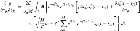
Plugging (13.39), (A.19), (A.24), (A.26) in (A.23) and taking expectation gives (A.22). Then, we compute
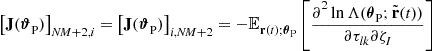 (A.27)
for ![]() , where
, where
![]() (A.28)
(A.28)
The new terms introduced by (A.28) are
![]() (A.29)
(A.29)
where ![]() is given in (13.38) and15
is given in (13.38) and15
 (A.30)
and
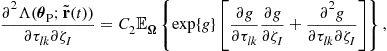 (A.31)
where ![]() is given in (13.38),
is given in (13.38), ![]() in (A.20),
in (A.20), ![]() in (A.30), and
in (A.30), and

Plugging (13.39), (A.19), (A.29), (A.31) in (A.28) and taking expectation gives (A.27). Next, we compute
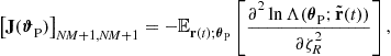 (A.32)
where
![]() (A.33)
(A.33)
The new term introduced by (A.33) is
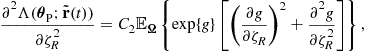 (A.34)
where ![]() is given in (13.38),
is given in (13.38), ![]() in (A.25), and
in (A.25), and

Plugging (13.39), (A.24), (A.34) in (A.33) and taking expectation, we obtain (A.32). Similarly, we compute
 (A.35)
where
![]() (A.36)
(A.36)
The new term introduced by (A.36) is
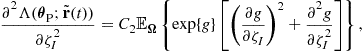 (A.37)
where ![]() is given in (13.38),
is given in (13.38), ![]() in (A.30) and
in (A.30) and
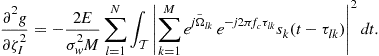
Plugging (13.39), (A.29), (A.37) into (A.36) and taking expectation gives (A.35). Finally, we compute
 (A.38)
![]() (A.39)
(A.39)
The new term introduced by (A.39) is
![]() (A.40)
(A.40)
where ![]() is given in (13.38),
is given in (13.38), ![]() in (A.25), and
in (A.25), and ![]() in (A.30). Plugging (13.39), (A.24), (A.29), (A.40) into (A.39) and taking expectation we obtain (A.38).
in (A.30). Plugging (13.39), (A.24), (A.29), (A.40) into (A.39) and taking expectation we obtain (A.38).
Now we compute the quantity
![]()
using ![]() and
and ![]() respectively given in (13.2) and (13.41)
respectively given in (13.2) and (13.41)
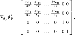 (A.41)
where ![]() and
and ![]() .
.
Relevant Theory: Signal Processing Theory Statistical Signal Processing, and Array Signal Processing
See Vol. 1, Chapter 4 Random Signals and Stochastic Processes
See Vol. 1, Chapter 11 Parametric Estimation
See Vol. 3, Chapter 7 Geolocation—Maps, Measurements, Models, and Methods
See Vol. 3, Chapter 8 Performance Analysis and Bounds
See Vol. 3, Chapter 19 Array Processing in the Face of Nonidealities
References
1. Bölcskei H, Paulraj AJ. Multiple-input multiple-output (MIMO) wireless systems. In: The Communications Handbook. second ed. CRC Press 2002;90.1–90.14.
2. Fishler E, Haimovich AM, Blum RS, Cimini L, Chizhik D, Valenzuela R. Spatial diversity in radars—models and detection performance. IEEE Trans Signal Process. 2006;54(3):823–838.
3. Li J, Stoica P. MIMO radar with colocated antennas. IEEE Signal Process Mag. 2007;24(5):106–114.
4. Haimovich AM, Blum RS, Cimini L. MIMO radar with widely separated antennas. IEEE Signal Process Mag. 2008;(1):116–129.
5. Blum RS. Limiting case of a lack of rich scattering environment for MIMO radar diversity. IEEE Signal Process Lett. 2009;16(10):901–904.
6. Aittomaki T, Koivunen V. Performance of MIMO radar with angle diversity under Swerling scattering model. IEEE J Sel Top Signal Process. 2010;4(1):101–114 (special issue on MIMO radar).
7. Grossi E, Lops M, Venturino L. Robust waveform design for MIMO radars. IEEE Trans Signal Process. 2011;59(7):3262–3271.
8. Akcakaya M, Nehorai A. MIMO radar sensitivity analysis for target detection. IEEE Trans Signal Process. 2011;59(7):3241–3250.
9. Yang Y, Blum RS. MIMO radar waveform design based on mutual information and minimum mean-square error estimation. IEEE Trans Aerosp Electron Syst. 2007;43:330–343.
10. He Q, Lehmann NH, Blum RS, Haimovich AM. MIMO radar moving target detection in homogeneous clutter. IEEE Trans Aerosp Electron Syst. 2010;46(3):1290–1301.
11. Godrich H, Haimovich AM, Blum RS. Target localization accuracy gain in MIMO radar based systems. IEEE Trans Inform Theory. 2010;56(6):2783–2803.
12. Sen S, Nehorai N. OFDM MIMO radar with mutual-information waveform design for low-grazing angle tracking. IEEE Trans Signal Process. 2010;58(6):3152–3162.
13. Niu R, Blum RS, Varshney PK, Drozd AL. Target tracking in widely separated non-coherent multiple-input multiple-output radar systems. In: Proceeding of the 43rd Asilomar Conference on Signals, Systems and Computers. November 2009;1181–1185.
14. Melvin ML. A STAP overview. IEEE Aerosp Electron Syst Mag. 2004;19(1):19–35.
15. Van Trees HL. Detection, Estimation, and Modulation Theory III: Radar-Sonar Signal Processing and Gaussian Signals in Noise. John Wiley & Sons Inc. 2001.
16. He Q, Blum RS. Noncoherent versus coherent MIMO radar: performance and simplicity analysis. Signal Process. 2012;92:2454–2463.
17. Poor HV. An Introduction to Signal Detection and Estimation. second ed. New York: Springer-Verlag; 1994.
18. He Q, Blum RS, Godrich H, Haimovich AM. Target velocity estimation and antenna placement for MIMO radar with widely separated antennas. IEEE J Sel Top Signal Process. 2010;4(1):79–100 (special issue on MIMO radar).
19. Woodward PM. Probability and Information Theory, with Applications to Radar. New York: McGraw-Hill; 1953.
20. Lehmann N, Haimovich AM, Blum RS, Cimini L. High resolution capabilities of MIMO radar. In: Proceeding of the 40th Asilomar Conference on Signal, System and Computers. November 2006;25–30.
21. San Antonio G, Fuhrmann DR, Robey FC. MIMO radar ambiguity functions. IEEE J Sel Top Signal Process. 2007;1(1):167–177.
22. Chen C, Vaidyanathan PP. MIMO radar ambiguity properties and optimization using frequency-hopping waveforms. IEEE Trans Signal Process. 2008;56(12):5926–5936.
23. Van Trees HL. Detection, Estimation, and Modulation Theory I. John Wiley & Sons Inc. 2001.
24. He Q, Blum RS, Haimovich AM. Noncoherent MIMO radar for location and velocity estimation: more antennas means better performance. IEEE Trans Signal Process. 2010;58(7):3661–3680.
25. He Q, Blum RS. Diversity gain for MIMO Neyman-Pearson signal detection. IEEE Trans Signal Process. 2011;59(3):869–881.
26. He Q, Blum RS. Cramer-Rao bound for MIMO radar target localization with phase errors. IEEE Signal Process Lett. 2010;17(1):83–86.
27. Godrich H, Haimovich AM, Poor HV. An analysis of phase synchronization mismatch sensitivity for coherent MIMO radar systems. In: Proceedings of the IEEE International Workshop on Computational Advances in Multi-Sensor Adaptive Processing, Aruba, Dutch Antilles. December 2009;153–156.
28. Godrich H, Haimovich AM. Localization performance of coherent MIMO radar systems subject to phase synchronization errors. In: Proceedings of the 4th International Symposium on Communications, Control and Signal Processing, Limassol, Cyprus, 3–5 March. 2010.
29. Akçakaya M, Nehorai A. MIMO Radar detection and adaptive design under a phase synchronization mismatch. IEEE Trans Signal Process. 2010;58(10):4994–5005.
30. Shakhguildyan VV, Sviridenko SS. Phase synchronization systems studies. IEEE Trans Commun COM-30 1982;(10):2260–2263.
31. Steinberg BD. Phase synchronizing a nonrigid, distributed, transmit-receive radar antenna array. IEEE Trans Aerosp Electron Syst AES-18 1982;(5):609–620.
32. E.H. Attia, Phase synchronizing large antenna arrays using the spatial correlation properties of radar clutter, Ph.D. Thesis, University of Pennsylvania, 1985.
33. Lee E-A, Dorny CN. A broadcast reference technique for self-calibrating of large antenna phased arrays. IEEE Trans Antennas Propag. 1989;37(8):1003–1010.
34. Willis NJ. Bistatic Radar. second ed. SciTech Publishing 2005.
35. Lopez-Dekker P, Mallorqui JJ, Serra-Morales P, Sanz-Marcos J. Phase synchronization and Doppler centroid estimation in fixed receiver bistatic SAR systems. IEEE Trans Geosci Remote Sens. 2008;46(11):3459–3471.
36. Ng BP, Lie JP, Er MH, Feng A. A practical simple geometry and gain/phase calibration technique for antenna array processing. IEEE Trans Antennas Propag. 2009;57(7):1963–1972.
37. Lindsey WC, Ghazvinian F, Hagmann WC, Dessouky K. Network synchronization. Proc IEEE. 1985;73(10):1445–1467.
38. Sundararaman B, Buy U, Kshemkalyani AD. Clock synchronization for wireless sensor networks: a survey. Ad Hoc Networks. 2005;3(3):281–323.
39. Tu Y, Pottie GJ. Coherent cooperative transmission from multiple adjacent antennas to a distant stationary antenna through AWGN channels. Proceedings of the IEEE Vehicular Technology Conference, AL, Spring. 2002;1:130–134.
40. Mudumbai R, Barriac G, Madhow U. On the feasibility of distributed beamforming in wireless networks. IEEE Trans Wireless Commun. 2007;6(4):1–10.
41. Li Q, Rus D. Global clock synchronization in sensor networks. In: Proceedings of the IEEE Conference on, Computer Communications. March 2004;564–574.
42. Brown DR, Prince G, McNeill JA. A method for carrier frequency and phase synchronization of two autonomous cooperative transmitters. In: Proceedings of the IEEE Workshop on Signal Processing Advances in Wireless Communications, New York. June 2005;260–264.
43. Brown III DR, Poor HV. Time-slotted round-trip carrier synchronization for distributed beamforming. IEEE Trans Signal Process. 2008;56(11):5630–5643.
44. Wang Q, Ren K. Time-slotted round-trip carrier synchronization in large-scale wireless networks. In: Proceedings of the IEEE International Conference on Communications. May 2008;5087–5091.
45. Yang Y, Blum RS. Phase synchronization for coherent MIMO radar: algorithms and their analysis. IEEE Trans Signal Process. 2011;59(11):5538–5557.
46. Olfati-Saber R, Fax JA, Murray RM. Consensus and cooperation in networked multi-agent systems. Proc IEEE. 2007;95(1):215–233.
47. Xiao L, Boyd S. Fast linear iterations for distributed averaging. System Control Lett. 2004;53:65–78.
48. Boyd S, Ghosh A, Prabhakar B, Shah D. Randomized gossip algorithms. IEEE Trans Inform Theory. 2006;52:2508–2530.
49. Xiao L, Boyd S, Kim S-J. Distributed average consensus with least-mean-square deviation. J Parallel Distr Comput. 2007;67(1):33–46.
50. Fagnani F, Zampieri S. Randomized consensus algorithms over large scale networks. IEEE J Sel Area Commun. 2008;26(4):634–649.
51. Aysal TC, Yildiz ME, Sarwate AD, Scaglione A. Broadcast gossip algorithms for consensus. IEEE Trans Signal Process. 2009;57:2748–2761.
52. Yang Y, Blum RS. Broadcast-based consensus with non-zero-mean stochastic perturbations. IEEE Trans Inform Theory 2013; In: <http://ieeexplore.ieee.org/stamp/stamp.jsp?tp=&arnumber=6459027>; 2013.
53. Schenato L, Gamba G. A distributed consensus protocol for clock synchronization in wireless sensor network. In: Proceedings of the 46th IEEE Conference on Decision and Control, New Orleans, LA. December 2007;2289–2294.
54. Xiong G, Kishore S. Analysis of distributed consensus time synchronization with Gaussian delay over wireless sensor networks. In: 2009;9. EURASIP J Wireless Commun Network. 2009 (Article ID 528161).
55. Rutman J. Characterization of phase and frequency instabilities in precision frequency sources: fifteen years of progress. Proc IEEE. 1978;66(9):1048–1075.
56. Demir A, Mehrotra A, Roychowdhury J. Phase noise in oscillators: a unifying theory and numerical methods. IEEE Trans Circ Syst Fund Theory Appl. 2000;47(5):655–674.
57. Skolnik MI, ed. Radar Handbook. second ed. New York: McGraw-Hill; 1990.
58. Levanon N, Mozeson E. Radar Signals. New York: John Wiley & Sons; 2004.
59. Yang Y, Blum RS. Minimax robust MIMO radar waveform design. IEEE J Sel Top Signal Process. 2007;1:147–155.
60. Yang Y, Blum RS, He ZS, Fuhrmann DR. MIMO radar waveform design via alternating projection. IEEE Trans Signal Process. 2010;58(3):1140–1445.
61. Naghibi T, Behnia F. MIMO radar waveform design in the presence of clutter. IEEE Trans Aerosp Electron Syst. 2011;47(2):770–781.
62. Chen C-Y, Vaidyanathan PP. MIMO radar waveform optimization with prior information of the extended target and clutter. IEEE Trans Signal Process. 2009;57(9):3533–3544.
63. Tang B, Tang J, Peng Y. MIMO radar waveform design in colored noise based on information theory. IEEE Trans Signal Process. 2010;58(9):4684–4697.
64. Zhang J, Wang H, Zhu X. Adaptive waveform design for separated transmit/receive ULA-MIMO radar. IEEE Trans Signal Process. 2010;58(9):4936–4942.
65. De Maio A, Lops M. Design principles of MIMO radar detectors. IEEE Trans Aerosp Electron Syst. 2007;43(3):886–898.
66. De Maio A, Lops M, Venturino L. Diversity-integration tradeoffs in MIMO detection. IEEE Trans Signal Process. 2008;56(10):5051–5061.
67. Fuhrmann DR, San Antonio G. Transmit beamforming for MIMO radar systems using signal cross-correlation. IEEE Trans Aerosp Electron Syst. 2008;44(1):171–186.
68. Friedlander B. Waveform design for MIMO radars. IEEE Trans Aerosp Electron Syst. 2007;43(3):1227–1238.
69. Li J, Stoica P, Xie Y. On probing signal design for MIMO radar. IEEE Trans Signal Process. 2007;55(8):4151–4161.
70. Naghibi T, Namvara M, Behniaa F. Optimal and robust waveform design for MIMO radars in the presence of clutter. IEEE Trans Signal Process. 2010;90(4):1103–1117.
71. Jajamovich GH, Lops M, Wang X. Space-time coding for MIMO radar detection and ranging. IEEE Trans Signal Process. 2010;58(12):6195–6206.
72. Aubry A, Lops M, Tulino AM, Venturino L. On MIMO detection under non-Gaussian target scattering. IEEE Trans Inform Theory. 2010;56(11):5822–5838.
73. Song X, Zhou S, Willett P. Reducing the waveform cross correlation of MIMO radar with space-time coding. IEEE Trans Signal Process. 2010;58(8):4213–4224.
74. Wang H, Liao G, Liu H, Li J, Lv H. Joint optimization of MIMO radar waveform and biased estimator with prior information in the presence of clutter. EURASIP J Adv Signal Process. 2011;2011:15.
75. Bell MR. Information theory and radar waveform design. IEEE Trans Inform Theory. 1993;39:1578–1597.
76. Cover TM, Thomas JA. Elements of Information Theory. New York: John Wiley & Sons; 1991.
77. Grenander U, Szegö G. Toeplitz Forms and Their Applications. second ed. New York: Chelsea Publishing Company; 1984.
78. Gray RM. Toeplitz and Circulant Matrices: A Review. 2002; In: http://www-ee.stanford.edu/gray/toeplitz.pdf; 2002.
79. Kassam SA, Poor HV. Robust techniques for signal processing: a survey. Proc IEEE. 1985;73(3):433–481.
1If we model the target as an antenna, we can define a target beamwidth based on its size using standard antenna array calculations.
2If the covariance matrix ![]() is not known, one may need to estimate it using secondary data. The readers are referred to literature on space-time adaptive processing (STAP) for more details [14].
is not known, one may need to estimate it using secondary data. The readers are referred to literature on space-time adaptive processing (STAP) for more details [14].
3Note that in this chapter, the integral over time in equations, such as (13.15) and (13.16) operates on each element of the corresponding matrix.
4To be more precise, the relationship is built upon the facts that the CRB depends on the mainlobe of the AF, and that the performance of the ML estimator tends to the CRB.
5Note that some of the open literature [21,22] may have different definitions for the MIMO radar AF.
6Assume the target has already been detected using a radar with a fairly coarse grid so we know the distances approximately, and one can develop specific relative values for variances for the reflection coefficients for different paths from transmit to receive antennas based on this.
7In [24] the authors have simulated a few cases where such assumptions do not exist and found similar results.
8Choosing an orthogonal set in a particular manner, say using the Karhunen-Loeve expansion [23], allows one to represent the received continuous signals by a set of random variables that compose a sufficient statistic for the target-absent versus target-present hypothesis testing problem.
9The notation![]() means
means![]() approaches
approaches![]() from right. Note that in the cases where
from right. Note that in the cases where![]() we will get no diversity gain.
we will get no diversity gain.
10In this section, we use the terms sensor, node, and element interchangely.
11![]() .
.
12Windowing can be applied in practice but we omit discussion of this well studied topic.
13Here we model the oscillator phase drift as varying slowly enough so as to be considered constant over any pulse train interval. We define noncoherent processing approaches as those approaches that do not require phase locking between the oscillators at all the different transmitter and receiver nodes.
14The ![]() means taking the real part of the quantity in the brackets.
means taking the real part of the quantity in the brackets.
15The ![]() means taking the imaginary part of the quantity in the brackets.
means taking the imaginary part of the quantity in the brackets.