
Space-Time Adaptive Processing for Radar
William L. Melvin, Georgia Institute of Technology, Atlanta, GA, USA, [email protected]
Abstract
Space-time adaptive processing (STAP) is an important radar technology. It is a cornerstone in the design of modern moving target indication and imaging radar systems. Specifically, STAP is a multidimensional filtering technique that mitigates the influence of clutter or radio frequency interference on principal radar products, viz. radar detections or images. This work serves as a tutorial reference of fundamental STAP concepts and techniques. The interested reader will encounter the basic STAP formulation, common STAP performance metrics, signal models, interference mitigation approaches, an application example corresponding to Doppler spread clutter mitigation in airborne radar systems, current challenges, and some implementation issues. The fundamentals presented herein are extensible to a range of radar signal processing problems.
Keywords
Space-time adaptive processing (STAP); Radar signal processing; Array processing; Radar detection; Radar clutter
2.12.1 Introduction
Space-time adaptive processing (STAP) is a two-dimensional, adaptive filtering technique foundational to modern radar system design and implementation. Generally, spatial sampling is given by the outputs of an array of antenna elements (sometimes called “channels”); the Fourier transform of space yields angle. There are essentially two time measurements in radar: fast-time and slow-time. Fast-time samples correspond to outputs of the analog-to-digital converter abiding with the Nyquist rate for the reflected radar waveform; the Fourier transform of fast-time is radio-frequency (RF), which relates to radar range. The processor collects slow-time voltage samples at a given range realization from distinct, reflected, pulsed transmissions; the Fourier transform of slow-time yields Doppler frequency. Depending on the statistical properties of the interference source, either slow-time or fast-time is applicable. For example, the adaptive suppression of ground clutter received by airborne or spaceborne radar requires joint spatial and slow-time adaptivity since clutter returns appear correlated in the angle-Doppler domain, but are uncorrelated in fast-time. Fast-time adaptive degrees of freedom play in role in wideband and terrain-bounce interference mitigation in both aerospace and surface-based radar systems.
Suppose we consider adaptive mitigation of Doppler-spread ground clutter returns in further detail. This problem arises in airborne and spaceborne radar systems searching for moving targets. The clutter returns are generally much stronger than the target signal, in many cases by orders of magnitude, thereby rendering detection in certain regions of the range-Doppler map virtually impossible using conventional antenna beamforming and Doppler processing techniques. Spatial and Doppler beamforming represent one-dimensional matched filtering operations. The matched filter maximizes signal-to-noise ratio (SNR), thereby maximizing probability of detection for a fixed false alarm rate for uncorrelated, circular Gaussian disturbance [1,2]. STAP is needed when clutter and radio frequency interference (RFI)—colored noise—are present; the STAP applies a space-time weighting incorporating estimated characteristics of the interference environment to asymptotically maximize signal-to-interference-plus-noise ratio (SINR), a sufficient condition to maximize the probability of detection for a fixed false alarm rate under the assumption the disturbance is circular Gaussian [3].
Fixed points on the Earth’s surface exhibit a Doppler frequency shift consistent with their angular displacement from the platform velocity vector, ![]() . In turn, this angular displacement corresponds to a specific angle of arrival at the antenna array. Thus, given a particular azimuth and elevation angle in the antenna coordinate system, the clutter Doppler frequency is precisely specified, and vice versa. The clutter angle-Doppler region of support is described as a ridge in airborne and spaceborne radar. This ridge is a line in sidelooking radar, opens up into an ellipse for varying degrees of platform yaw, and becomes a circle for the forward-looking array. Figure 12.1 provides example power spectral density (PSD) and minimum variance distortionless response (MVDR) super-resolution plots of the clutter angle-Doppler region of support for the side-looking array radar (SLAR), a forward-looking array radar (FLAR), and an array with forty-five (45)° of yaw. Typical radar parameters are used in this example and will be described in further detail in subsequent sections.
. In turn, this angular displacement corresponds to a specific angle of arrival at the antenna array. Thus, given a particular azimuth and elevation angle in the antenna coordinate system, the clutter Doppler frequency is precisely specified, and vice versa. The clutter angle-Doppler region of support is described as a ridge in airborne and spaceborne radar. This ridge is a line in sidelooking radar, opens up into an ellipse for varying degrees of platform yaw, and becomes a circle for the forward-looking array. Figure 12.1 provides example power spectral density (PSD) and minimum variance distortionless response (MVDR) super-resolution plots of the clutter angle-Doppler region of support for the side-looking array radar (SLAR), a forward-looking array radar (FLAR), and an array with forty-five (45)° of yaw. Typical radar parameters are used in this example and will be described in further detail in subsequent sections.
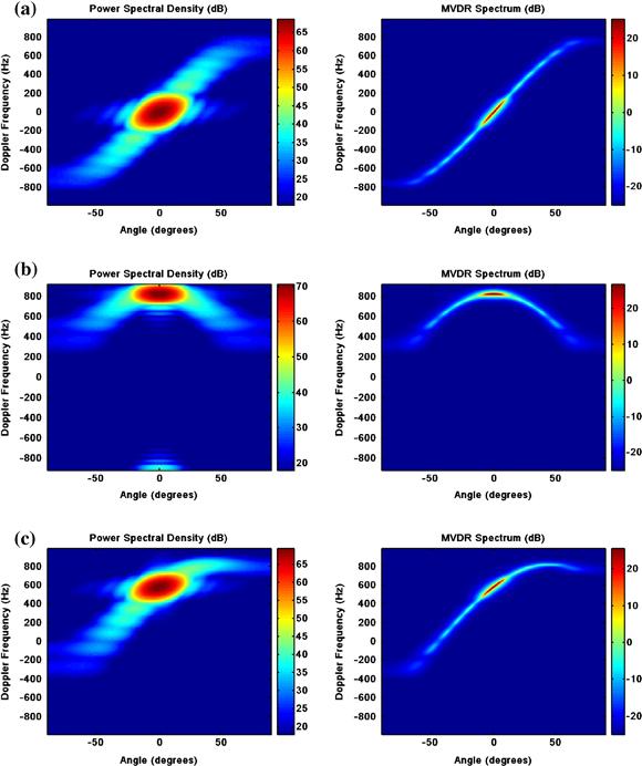
Figure 12.1 Clutter angle-Doppler region of support for three array configurations. (a) PSD (left) and super-resolution clutter image (right) for side-looking array, (b) PSD (left) and super-resolution clutter image (right) for forward-looking array, and (c) PSD (left) and super-resolution clutter image (right) for array with 45° of yaw.
The PSD plots are a result of classical, two-dimensional, Fourier analysis. Resolution is limited in Fourier analysis by roughly the wavelength of the signal divided by the aperture length; to resolve more closely spaced signals, either the wavelength must be decreased for a fixed aperture size, or the physical aperture must be increased for a fixed wavelength. Super-resolution spectral estimators overcome the diffraction limitations of Fourier-based methods, oftentimes providing resolution enhancement by a factor of two to five, or even more. It turns out that STAP is intimately related to the MVDR spectrum, as discussed in Section 2.12.2.2.2. Hence, STAP likewise exhibits super-resolution properties, enabling it to detect slow moving targets buried in mainbeam clutter or targets closely spaced to other interference sources.
As mentioned, STAP coherently combines spatial and temporal voltage samples from a particular range realization using a data-dependent weighting to maximize SINR. The corresponding adaptive filter frequency response exhibits sharp nulls along the clutter region of support while maximizing the gain at another, specified angle-Doppler location where a potential target might exist. A target with a Doppler frequency outside of the mainlobe clutter Doppler spread (given as the highest power, circular region in the PSD) is called exoclutter, whilst targets within the mainlobe clutter spread are endoclutter. The STAP frequency response null is the inverse of the super-resolution contour shown in Figure 12.1. Hence, STAP itself exhibits super-resolution properties, providing detection performance within the diffraction limits of the traditional space-time aperture. This important characteristic makes STAP invaluable on airborne and spaceborne platforms, enabling drastic reduction in antenna aperture length for a desired minimum detectable velocity (MDV). The asymptotic STAP frequency responses for each of the PSDs in Figure 12.1 are given in Figure 12.2. (The asymptotic STAP response is optimal, since this is the weighting that precisely maximizes SINR.) The filter is tuned to broadside and 400 Hz Doppler.
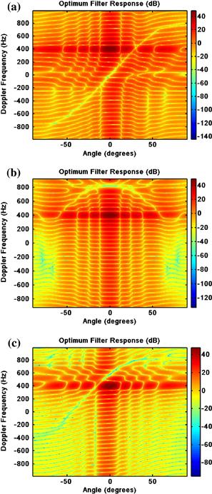
Figure 12.2 Comparison of STAP frequency response for the three scenarios in Figure 12.1. (a) Side-looking array, (b) forward-looking array, and (c) array with 45° of yaw.
The MDV is the lowest target range-rate where sufficient SINR exists to permit a specified probability of detection for an acceptable probability of false alarm. Conversely, the MDV occurs at those points where the loss in SINR due to clutter is maximally acceptable. Figure 12.3 provides an example of the loss in SINR due to clutter for the radar array configuration of Figures 12.1 and 12.2. SINR loss will be described further in Section 2.12.2. Noise-limited performance is at 0 dB. The depth of the loss null is related to the clutter-to-noise ratio (CNR).

2.12.1.1 Historical overview
Historical overviews of STAP are given in [4,5]. Reed [4] describes the earlier history of adaptive arrays, whilst Klemm [5] covers more contemporary developments in STAP. Additionally, Entzminger et al. [6] discusses the history and future of Joint STARS and ground moving target indication (GMTI), identifying the central role of STAP in the success of both.
Table 12.1 is an historical accounting of STAP from the author’s perspective, as well as information derived from [4–6]. As such, it attempts to convey some key developments and general trends, but is necessarily incomplete. (Note: references to specific works are provided throughout the remainder of this text. Additionally, Klemm [5] provides an excellent, historical accounting and perspective, and is highly recommended to the interested reader.)
Table 12.1
Some Significant Events in the History of STAP
| Year | Topic |
| 1957 | Paul Howells of General Electric, Syracuse (now Lockheed-Martin), develops technique to electronically scan antenna null in direction of a jammer |
| 1959 | Howells receives US Patent, “Intermediate frequency side-lobe canceller” |
| 1962 | Howells and Sidney Applebaum successfully test five-loop side-lobe canceller |
| 1963 | Howells and Applebaum, at Syracuse University Research Corp. (then Syracuse Research Corp., now SRC) investigate application of adaptive techniques to radar, including OTHR and BMD radar |
| 1965 (1976) | Applebaum publishes “Adaptive Arrays,” SURC TR-66–001, later available in IEEE Transactions on Antennas and Propagation in 1976 |
| 1969 | Lloyd Griffiths publishes an adaptive algorithm for wideband antennas in Proceedings of the IEEE |
| 1969 | V. Anderson, H. Cox and N. Owsley separately publish works on adaptive arrays for sonar |
| 1971 | R.T. Compton describes the application of adaptive arrays for communications systems in Ohio State University Quarterly Rept. 3234–1, December 1971 |
| 1972 | O.L. Frost publishes an adaptive algorithm for antenna arrays incorporating constraints |
| 1972 | Howells and Applebaum investigate adaptive radar for Airborne Early Warning (AEW) radar |
| 1973 | Larry Brennan and Irving Reed publish the seminal paper, “Theory of adaptive radar,” in IEEE Trans. AES |
| 1974 | Reed, John Mallett and Brennan publish a paper describing the Sample Matrix Inverse (SMI) method for adaptive arrays in IEEE Transactions on Aerospace and Electronic Systems |
| 1976 | “Adaptive antenna systems,” published by Bernard Widrow et al. in IEEE Proceedings |
| 1980 | R.A. Monzingo and T.W. Miller publish the book Adaptive Arrays |
| 1983 | Rule for calculating clutter subspace dimension proposed by Richard Klemm in IEEE Proceedings Part F, Vol 130, February 1983 |
| 1991 | Joint STARS prototypes deploy to Gulf War using adaptive clutter suppression methods (1978, Pave Mover was pre-cursor) |
| 1992 | Klemm proposes spatial transform techniques for dimensionality reduction in paper on antenna design for STAP |
| 1992 | Real-time STAP implementation by Alfonso Farina et al. |
| 1992 | Bob DiPietro presents post-Doppler STAP algorithm at Asilomar Conference on Signals, Systems and Computers |
| 1994 | Post-Doppler, beamspace method proposed by Wang and Cai in IEEE Transactions on Aerospace and Electronic Systems |
| 1994 | Jim Ward of MIT Lincoln Lab describes STAP techniques in ESC-TR-94–109, Space–Time Adaptive Processing for Airborne Radar |
| 1995 | Air Force Rome Laboratory (now Air Force Research Laboratory) and Westinghouse (now Northrop Grumman) collect twenty-four channel airborne radar data for STAP research and development under the Multichannel Airborne Radar Measurements (MCARM) program |
| 1998 | Richard Klemm publishes first STAP text book, Space-Time Adaptive Processing: Principles and Applications |
| 1999 | IEE Electronics and Communications Engineering Journal (ECEJ) Special Issue on STAP (Klemm, Ed.) |
| 1999 | STAP techniques for space-based radar, by Rabideau and Kogon, presented at IEEE Radar Conference |
| 1999 | 3-D STAP for hot and cold clutter mitigation appears in IEEE Trans. AES by Techau, Guerci, Slocumb and Griffiths |
| 2000 | Bistatic STAP techniques appear in literature (numerous authors) |
| 2000 | IEEE Transactions on Aerospace and Electronic Systems Special Section on STAP (William Melvin, Ed.) |
| 2002 | DARPA’s Knowledge-Aided Sensor Signal Processing & Expert Reasoning (KASSPER) commences under leadership of Joseph Guerci |
| 2003 | Guerci publishes the book Space-Time Adaptive Processing for Radar |
| 2004 | IEE publishers release the book The Applications of Space-Time Processing (Klemm, Ed.) |
| c. 2005 | Multi-Input, Multi-Output (MIMO) adaptive systems (numerous authors) |
| 2006 | IEEE Transactions on Aerospace and Electronic Systems, Special Section on Knowledge-Aided Signal and Data Processing (Melvin, Guerci, Ed.) |
| 2009 | Cognitive Radar (Guerci) |
2.12.1.2 Organization
We organize the remaining discussion as follows:
• Section 2.12.2 describes basic concepts, include target detection; different space-time optimal filter formulations, including the maximum SINR filter, the minimum variance beamformer, and the generalized sidelobe canceler; the sample matrix inversion (SMI) approach to adaptive filtering; and, key performance metrics, such as SINR loss.
• Section 2.12.3 discusses clutter, RFI, target, and receiver space-time signal models.
• Section 2.12.4 discusses different adaptive filter topologies, including several reduced-rank methods, reduced-dimension STAP, and parametric adaptive matched filtering.
• Section 2.12.5 describes the utility of STAP to clutter suppression in airborne radar, as an example. This section also includes benchmark results for some of the algorithms discussed in Section 2.12.4.
• Much of current STAP research focuses on extending textbook discussion to real-world application. Section 2.12.6 describes various STAP challenges and research areas, including the impact of heterogeneous or nonstationary clutter on detection performance and mitigating techniques, application to airborne bistatic and conformal array radar, and knowledge-aided STAP. Each of these challenge areas predominantly focuses on issues surrounding effective estimation of the interference covariance matrix.
• A description of some additional, practical issues in STAP implementation is given in Section 2.12.7, including maximum likelihood angle estimation and adaptive matched filter normalization.
• In Section 2.12.8 we briefly discuss some multichannel radar data collection efforts.
• Summary comments are given in Section 2.12.9, along with notation and acronym lists in the appendices.
2.12.1.3 Key points
STAP is a key component of modern radar. Some important points are given below:
• STAP is really a catch-all phrase for a variety of weight calculation schemes and adaptive architectures.
• Radar terminology usually includes two time measurements: fast-time, corresponding to a sample rate consistent with the analog-to-digital converter clock speed and effectively measuring range; and, slow-time, where the pulse repetition interval (PRI) defines the sample rate and separating targets and clutter in Doppler frequency is the primary motivation. Space and slow-time are used to mitigate ground clutter returns in aerospace radar, whereas space and fast-time are used to cope with wideband RFI or multipath signals in aerospace or surface radar systems.
• Herein, we focus on space and slow-time adaptive processing for clutter suppression. The ideas discussed are easily extended to other radar degrees of freedom (DoFs), include fast-time, polarization, and multiple passes.
• Implementation of the optimal processor requires precise knowledge of the null-hypothesis covariance matrix and the target space-time steering vector. The adaptive filter is an approximation to the optimal processor, since neither covariance matrix nor steering vector are known in practice. There are two primary factors leading to differences between adaptive and optimal filter outputs: covariance matrix estimation error and unknown array manifold due to amplitude and phase error as a function of frequency. Adaptive SINR loss describes the impact of both of these errors on detection performance potential.
• Current STAP research focuses on coupling basic STAP theory, physics-based models, and the realities of the real-world operating environment to construct practical detection architectures.
• STAP is applied at the coherent processing interval (CPI) level, often typically prior to noncoherent—or post-detection—integration. Maximizing SINR is always effective at improving detection performance, since the separation between the null and alternative hypothesis output probability density functions increases.
• In many respects, STAP development is in its early stages, at least from an implementation perspective. It has been only recently that embedded computing power has improved to the point where more flexible, real-time STAP implementation is feasible.
2.12.2 Basic concepts
In this section we discuss radar space-time detection and several approaches to calculate the optimal space-time weight vector: the maximum SINR filter, the minimum variance beamformer, the generalized sidelobe canceler, and use of the Rayleigh quotient and generalized eigen-analysis. We introduce the sample matrix inverse adaptive filter as the most common of the various adaptive implementations used in radar application. We also discuss several important STAP metrics, such as clairvoyant and adaptive SINR loss and improvement factor.
2.12.2.1 Detection
Suppose we collect M spatial samples across the antenna array for range realization k and each of the N received pulses. These voltages are organized in a vector as
![]() (12.1)
(12.1)
where ![]() is the space-time snapshot and
is the space-time snapshot and ![]() is the spatial snapshot for the nth pulse. Two hypotheses correspond to (12.1): the null hypothesis,
is the spatial snapshot for the nth pulse. Two hypotheses correspond to (12.1): the null hypothesis, ![]() , where only additive interference and noise are present; and, the alternative hypothesis,
, where only additive interference and noise are present; and, the alternative hypothesis, ![]() , which includes target presence in addition to the components of the null hypothesis. Defining
, which includes target presence in addition to the components of the null hypothesis. Defining ![]() as the clutter space-time snapshot,
as the clutter space-time snapshot, ![]() as the RFI space-time snapshot,
as the RFI space-time snapshot, ![]() as the uncorrelated noise space-time snapshot, and
as the uncorrelated noise space-time snapshot, and ![]() the target space-time snapshot, we have
the target space-time snapshot, we have
![]() (12.2)
(12.2)
The radar detection problem is to decide, given ![]() , which of the two hypotheses is most probable. It is shown in [3] that maximizing SINR is equivalent to maximizing probability of detection for a fixed false alarm rate when
, which of the two hypotheses is most probable. It is shown in [3] that maximizing SINR is equivalent to maximizing probability of detection for a fixed false alarm rate when ![]() is jointly complex normal with zero mean and covariance matrix,
is jointly complex normal with zero mean and covariance matrix, ![]() , viz.
, viz. ![]() . We wish to combine the elements of
. We wish to combine the elements of ![]() using a linear, finite impulse response (FIR) filter, and compare the scalar to a threshold,
using a linear, finite impulse response (FIR) filter, and compare the scalar to a threshold, ![]() , to decide which hypothesis is a best fit,
, to decide which hypothesis is a best fit,
 (12.3)
where ![]() is the space-time weight vector.
is the space-time weight vector.
Figure 12.4 shows probability of detection, ![]() , as a function of output SINR for varying probability of false alarm,
, as a function of output SINR for varying probability of false alarm, ![]() . The curves correspond to nonfluctuating and Swerling 1 target types for
. The curves correspond to nonfluctuating and Swerling 1 target types for ![]() and
and ![]() . As seen,
. As seen, ![]() increases monotonically with SINR. Also, it is seen that for reasonably high
increases monotonically with SINR. Also, it is seen that for reasonably high ![]() we generally need higher SINR to detect a Swerling 1 target at the same rate as the nonfluctuating target due to fading; the SINR difference between Swerling 1 and nonfluctating detection curves is called fluctuation loss.
we generally need higher SINR to detect a Swerling 1 target at the same rate as the nonfluctuating target due to fading; the SINR difference between Swerling 1 and nonfluctating detection curves is called fluctuation loss.

2.12.2.2 Space-time filter formulations
2.12.2.2.1 Maximum SINR filter
A primary objective in STAP is to approximate as closely as possible the optimal weighting that maximizes SINR. By attempting to maximize output SINR, the STAP maximizes the probability of detection for a fixed false alarm rate, as discussed in the prior section. We now formulate the optimal weight vector.
The target snapshot is of the form, ![]() , where
, where ![]() is a complex gain term proportional to the square root of the target cross section,
is a complex gain term proportional to the square root of the target cross section, ![]() is the space-time steering vector of dimension NM-by-one,
is the space-time steering vector of dimension NM-by-one, ![]() is azimuth,
is azimuth, ![]() is elevation, and
is elevation, and ![]() is Doppler frequency. In the nonfluctuating target case,
is Doppler frequency. In the nonfluctuating target case, ![]() is a constant, whereas in the Swerling 1 case,
is a constant, whereas in the Swerling 1 case, ![]() , where
, where ![]() is the target signal variance [1,7,8]. The space-time steering vector is the Kronecker product of the spatial steering vector,
is the target signal variance [1,7,8]. The space-time steering vector is the Kronecker product of the spatial steering vector, ![]() , and the temporal steering vector,
, and the temporal steering vector, ![]() . Generally, the spatial steering vector describes the phase variation among the spatial antenna channels (of common size and gain) to a signal with a direction of arrival of
. Generally, the spatial steering vector describes the phase variation among the spatial antenna channels (of common size and gain) to a signal with a direction of arrival of ![]() , whereas the temporal steering vector describes the phase variation over the slow-time aperture to a signal with a particular range-rate [9–11]. If the aperture in either space or time is uniformly sampled, the corresponding steering vector will be Vandermonde.
, whereas the temporal steering vector describes the phase variation over the slow-time aperture to a signal with a particular range-rate [9–11]. If the aperture in either space or time is uniformly sampled, the corresponding steering vector will be Vandermonde.
The output SINR of the FIR filter with weight vector, ![]() , is the ratio of target power,
, is the ratio of target power, ![]() , to interference-plus-noise power,
, to interference-plus-noise power, ![]() , given as
, given as
 (12.4)
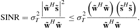
Using the definition for ![]() gives,
gives, ![]() , and the Schwarz Inequality lets us write (12.4) as
, and the Schwarz Inequality lets us write (12.4) as
 (12.5)
In this case, ![]() and
and ![]() . By inspection, we find that the right side of the inequality achieves the upper bound when
. By inspection, we find that the right side of the inequality achieves the upper bound when ![]() , thereby providing the solution for the optimal weight vector. Through substitution, it follows that
, thereby providing the solution for the optimal weight vector. Through substitution, it follows that
![]() (12.6)
(12.6)
for arbitrary scalar, ![]() , is the weighting that yields maximal output SINR. When the disturbance is uncorrelated noise,
, is the weighting that yields maximal output SINR. When the disturbance is uncorrelated noise, ![]() , where
, where ![]() is the noise power; then, (12.6) becomes the space-time matched filter, viz.
is the noise power; then, (12.6) becomes the space-time matched filter, viz. ![]() .
.
Inserting the optimal weight vector, ![]() , into (12.4) yields the maximum output SINR,
, into (12.4) yields the maximum output SINR,
![]() (12.7)
(12.7)
For simplicity, and without loss in meaning, in subsequent sections we use ![]() .
.
The maximum SINR weight vector has the following interpretation. If ![]() , then
, then ![]() is the whitened data vector, where
is the whitened data vector, where ![]() and
and ![]() is the NM-by-NM identity matrix. This results because
is the NM-by-NM identity matrix. This results because
![]() (12.8)
(12.8)
Then, the filter employing the maximum SINR weight vector is seen as a cascade of whitening and warped matched filtering operations,
![]() (12.9)
(12.9)
where ![]() is the warped matched filter accounting for the linear transformation of the target signal through the whitening process and
is the warped matched filter accounting for the linear transformation of the target signal through the whitening process and ![]() is the original matched filter weight vector.
is the original matched filter weight vector.
2.12.2.2.2 Minimum variance beamformer
The minimum variance (MV) space-time beam former is another common formulation leading to the adaptive processor [12,13]. The MV beamformer employs a weight vector yielding minimal output power subject to a linear constraint on the desired target spatial and temporal response:
![]() (12.10)
(12.10)
where g is a complex scalar. We can determine the weight vector satisfying the problem statement in (12.10) using the method of Lagrange. Thus, define the following cost function
![]() (12.11)
(12.11)
where ![]() is a complex Lagrangian multiplier and
is a complex Lagrangian multiplier and ![]() . Taking the gradient of (12.11) with respect to the conjugate of the weights and setting to zero gives
. Taking the gradient of (12.11) with respect to the conjugate of the weights and setting to zero gives
![]() (12.12)
(12.12)
Solving (12.12) for the weight vector yields
![]() (12.13)
(12.13)
Next, we find by applying the constraint in (12.10) that
![]() (12.14)
(12.14)
Solving (12.14) for ![]() then gives
then gives
![]() (12.15)
(12.15)
The minimum variance weight vector follows from (12.13) and (12.15) as
 (12.16)
Equation (12.16) abides by the form ![]() , where
, where
![]() (12.17)
(12.17)
Hence, (12.16) likewise yields maximal SINR.
Setting ![]() is known as the distortionless response, and the corresponding weight vector yields the minimum variance distortionless response (MVDR) beamformer. The output power of the MVDR beamformer is given as
is known as the distortionless response, and the corresponding weight vector yields the minimum variance distortionless response (MVDR) beamformer. The output power of the MVDR beamformer is given as
![]() (12.18)
(12.18)
The MVDR spectrum, as given in Figure 12.1, follows from (12.18) by scanning the space-time steering vector in the denominator over the angle and Doppler locations of interest.
2.12.2.2.3 Generalized sidelobe canceler
The GSLC is a formulation that conveniently converts the minimum variance constrained beamformer described in the preceding section into an unconstrained form [12,14]. Many prefer the GSLC interpretation of STAP over the whitening filter-warped matched filter interpretation of Section 2.12.2.2.1; since the GSLC implements the MV beamformer for the single linear constraint [14], this structure likewise can be shown to maximize output SINR.
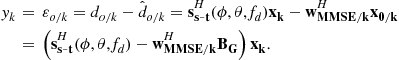
Figure 12.5 provides a block diagram of the GSLC. The top leg of the GSLC generates a quiescent response by forming a beam at the angle and Doppler of interest. A blocking matrix, ![]() , prevents the target signal from entering the lower leg; essentially, the blocking matrix forms a notch filter tuned to
, prevents the target signal from entering the lower leg; essentially, the blocking matrix forms a notch filter tuned to ![]() . With the desired signal absent from the lower leg, the processor tunes the weight vector to provide a minimal mean square error (MMSE) estimate of the interference in the top leg. In the final step, the processor differences the desired signal,
. With the desired signal absent from the lower leg, the processor tunes the weight vector to provide a minimal mean square error (MMSE) estimate of the interference in the top leg. In the final step, the processor differences the desired signal, ![]() , with the estimate from the lower leg,
, with the estimate from the lower leg, ![]() , to form the filter output,
, to form the filter output, ![]() . Ideally, any large residual at the output corresponds to an actual target.
. Ideally, any large residual at the output corresponds to an actual target.
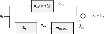
The desired signal is given as
![]() (12.19)
(12.19)
The signal vector in the lower leg is
![]() (12.20)
(12.20)
Forming the quiescent response of (12.19) uses a single degree of freedom (DoF), resulting in the reduced dimensionality of ![]() . By weighting the signal vector in the lower leg, the GSLC forms a MMSE estimate of
. By weighting the signal vector in the lower leg, the GSLC forms a MMSE estimate of ![]() as
as
![]() (12.21)
(12.21)
where the MMSE weight vector follows from the well-known Wiener-Hopf equation [12,13],
![]() (12.22)
(12.22)
The lower leg covariance matrix is
![]() (12.23)
(12.23)
whilst the cross-correlation between lower and upper legs is
![]() (12.24)
(12.24)
The GSLC filter output is then
 (12.25)
Comparing (12.25) and (12.3), we identify
![]() (12.26)
(12.26)
We compute the output SINR as the ratio of output signal power to interference-plus-noise power, as in (12.4). The signal-only output power of the GSLC is
 (12.27)
and the output interference-plus-noise power is
![]() (12.28)
(12.28)
The ratio of (12.27) and (12.28) is
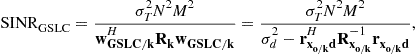 (12.29)
where ![]() . We arrive at the denominator in (12.29) by using (12.22)–(12.24),
. We arrive at the denominator in (12.29) by using (12.22)–(12.24),
 (12.30)
2.12.2.2.4 Rayleigh quotient
The optimal weight vector in Section 2.12.2.2.1 maximizes SINR. As seen from (12.4), for weight vector ![]() , SINR is given as the ratio of quadratics,
, SINR is given as the ratio of quadratics, ![]() . Thus, our problem is to find the weight vector that maximizes this function. In accord with [15], and similar to our discussion in Section 2.12.2.2.1, SINR is written as
. Thus, our problem is to find the weight vector that maximizes this function. In accord with [15], and similar to our discussion in Section 2.12.2.2.1, SINR is written as
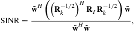 (12.31)
where ![]() . The weight vector,
. The weight vector, ![]() , that maximizes this Rayleigh quotient form is known to be proportional to the eigenvector
, that maximizes this Rayleigh quotient form is known to be proportional to the eigenvector ![]() associated with the largest eigenvalue
associated with the largest eigenvalue ![]() of the matrix in the numerator [13],
of the matrix in the numerator [13],
![]() (12.32)
(12.32)
and so
![]() (12.33)
(12.33)
Take the case where ![]() , as previously introduced in Section 2.12.2.2.1. The maximum eigenvector in (12.32) must abide by
, as previously introduced in Section 2.12.2.2.1. The maximum eigenvector in (12.32) must abide by
![]() (12.34)
(12.34)
The solution for ![]() in (12.34) is thus seen to be
in (12.34) is thus seen to be
![]() (12.35)
(12.35)
and so, as expected,
![]() (12.36)
(12.36)
(Note: inserting (12.35) in (12.34) gives ![]() times a scalar on each side of the equation, thereby satisfying the eigen-relation.)
times a scalar on each side of the equation, thereby satisfying the eigen-relation.)
By plugging ![]() found in (12.33) into (12.4), it is straightforward to show that the maximum SINR is equal to
found in (12.33) into (12.4), it is straightforward to show that the maximum SINR is equal to ![]() . In this vein, using (12.35) in (12.34) gives
. In this vein, using (12.35) in (12.34) gives
![]() (12.37)
(12.37)
which is the desired result and matches the expression given in (12.7).
2.12.2.2.5 Generalized eigen-analysis
The second approach, described in [13], begins by noting that the solution to maximizing SINR is equivalent to finding the maximum eigenvalue and associated eigenvector for the generalized Eigen-problem
![]() (12.38)
(12.38)
This can be solved as an ordinary eigen-equation by writing it as
![]() (12.39)
(12.39)
Then, the weight vector that maximizes (12.4) is proportional to the eigenvector ![]() associated with the largest eigenvalue
associated with the largest eigenvalue ![]() of
of ![]() ,
,
![]() (12.40)
(12.40)
The maximum eigenvalue of ![]() is the maximum achievable SINR in (12.4).
is the maximum achievable SINR in (12.4).
If we again consider the case where ![]() , the generalized eigen-analysis equation of (12.39) becomes
, the generalized eigen-analysis equation of (12.39) becomes
![]() (12.41)
(12.41)
which, we find, is satisfied when ![]() . Substituting this eigenvector,
. Substituting this eigenvector, ![]() , into (12.41) gives,
, into (12.41) gives,
![]() (12.42)
(12.42)
from which it is seen the maximum eigenvalue, ![]() , is identical to the result in (12.37) and also the same as the maximum SINR expression found in Section 2.12.2.2.1.
, is identical to the result in (12.37) and also the same as the maximum SINR expression found in Section 2.12.2.2.1.
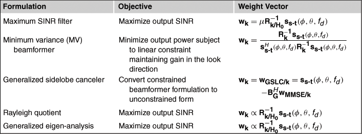
2.12.2.2.6 Summary
Table 12.2 summarizes the weight vector formulation given in the prior sections.
2.12.2.3 Sample matrix inversion
All of the previously described approaches to filter design presume the availability of the interference-plus-noise covariance matrix for the kth realization, ![]() , and perfectly known target space-time steering vector,
, and perfectly known target space-time steering vector, ![]() . In practice, neither
. In practice, neither ![]() nor
nor ![]() is known. The disturbance covariance matrix,
is known. The disturbance covariance matrix, ![]() , changes as look-angle, platform location, and platform attitude change. Errors in
, changes as look-angle, platform location, and platform attitude change. Errors in ![]() are generally a result of straddling the precise target spatial or temporal frequency when searching over angle and Doppler, as well as system hardware errors that most greatly affect the spatial component,
are generally a result of straddling the precise target spatial or temporal frequency when searching over angle and Doppler, as well as system hardware errors that most greatly affect the spatial component, ![]() . These system errors generally manifest as spatially varying, complex gain errors due to factors such as spatial variation in element gain patterns, varying line lengths, radome and airframe interactions, etc.
. These system errors generally manifest as spatially varying, complex gain errors due to factors such as spatial variation in element gain patterns, varying line lengths, radome and airframe interactions, etc.
A number of techniques are available to adapt the weight vector, including least means square (LMS) and recursive least squares (RLS) formulations [12]. However, the sample matrix inversion (SMI) method is by far the most popular choice for radar application for two primary reasons: (1) convergence of the SMI approach depends only on the number of samples used to estimate the unknown interference-plus-noise covariance matrix, regardless of environmental conditions as long as the data are independent and identically distributed (IID), for a system of specified DoFs; and, (2) prior to processing, radar systems generally collect their data in blocks, called coherent processing intervals (CPIs), and so a batch processing strategy using SMI is fully acceptable. In the SMI approach, the optimal weight vector,
![]() (12.43)
(12.43)
is simply replaced with the adaptive weight vector,
![]() (12.44)
(12.44)
where ![]() is a scalar that often depends on estimated quantities,
is a scalar that often depends on estimated quantities, ![]() is the interference-plus-noise covariance matrix estimate, and
is the interference-plus-noise covariance matrix estimate, and ![]() is the hypothesized space-time steering vector. In the absence of straddle error, system errors dominate the error between
is the hypothesized space-time steering vector. In the absence of straddle error, system errors dominate the error between ![]() and
and ![]() . Generally, array errors are explicitly modeled as
. Generally, array errors are explicitly modeled as
![]() (12.45)
(12.45)
where ![]() is the spatially-varying error between the ideal and actual array manifold, and
is the spatially-varying error between the ideal and actual array manifold, and ![]() and
and ![]() are Kronecker (tensor) and Hadamard (element-wise) products, respectively.
are Kronecker (tensor) and Hadamard (element-wise) products, respectively.
In practice, ![]() is “calibrated out” of the system using a variety of techniques, including array tuning on an antenna range or in situ using the clutter background and navigation data to estimate differences between ideal and actual multi-channel antenna responses [16]. Correspondingly, the hypothesized space-time steering vector is then
is “calibrated out” of the system using a variety of techniques, including array tuning on an antenna range or in situ using the clutter background and navigation data to estimate differences between ideal and actual multi-channel antenna responses [16]. Correspondingly, the hypothesized space-time steering vector is then
![]() (12.46)
(12.46)
where ![]() is an estimate of the array error vector, and
is an estimate of the array error vector, and ![]() and
and ![]() are otherwise the hypothesized temporal and spatial steering vectors accounting for potential straddle. Temporal errors due to system non-ideality are commonly very small for the typical STAP CPI, and thus usually are not considered further.
are otherwise the hypothesized temporal and spatial steering vectors accounting for potential straddle. Temporal errors due to system non-ideality are commonly very small for the typical STAP CPI, and thus usually are not considered further.
The complex baseband, pulse compressed, space-time snapshots comprise the voltage vectors for the pth CPI,
![]() (12.47)
(12.47)
A particular realization, ![]() , chosen from amongst the space-time vectors in (12.47) for filtering and detection thresholding is called the cell-under-test (CUT); multiple CUTs form the primary data set. The remaining vectors in (12.47) are available to estimate the unknown interference-plus-noise covariance matrix and are called training or secondary data. The primary data set can be as small as a single CUT with several adjacent realizations serving as guard cells; the purpose of the guard cell region is to prevent any target energy from leaking into the training interval. Let
, chosen from amongst the space-time vectors in (12.47) for filtering and detection thresholding is called the cell-under-test (CUT); multiple CUTs form the primary data set. The remaining vectors in (12.47) are available to estimate the unknown interference-plus-noise covariance matrix and are called training or secondary data. The primary data set can be as small as a single CUT with several adjacent realizations serving as guard cells; the purpose of the guard cell region is to prevent any target energy from leaking into the training interval. Let ![]() be the number of guard cells on either side of the primary data region. Then, define the training set as
be the number of guard cells on either side of the primary data region. Then, define the training set as
![]() (12.48)
(12.48)
It is shown in [17] that if the data vectors comprising the training interval—the columns of (12.48)—are IID with respect to the null-hypothesis of the CUT, a maximum likelihood estimate for ![]() is
is
![]() (12.49)
(12.49)
A fundamental question centers on how many training samples, ![]() , lead to an acceptable covariance matrix estimate. This matter was addressed in [17] and considered in further detail in Section 2.12.2.4.2.
, lead to an acceptable covariance matrix estimate. This matter was addressed in [17] and considered in further detail in Section 2.12.2.4.2.
2.12.2.4 Metrics
In radar, performance is generally measured according to the specific goals of the collection and processing mode. In moving target indication (MTI) radar, probability of detection, ![]() , and false alarm rate (FAR)—or probability of false alarm,
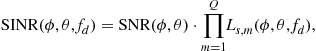
, and false alarm rate (FAR)—or probability of false alarm, ![]() —are the primary measures of performance. As discussed in Section 2.12.2.1, the probability of detection is a monotonic function of output SINR for a fixed false alarm rate. Thus, measures of SINR are key to understanding achievable system performance. Among these measures, SINR loss metrics are preferable, since they characterize performance over certain independent variables—usually range rate or Doppler frequency, as shown in Figure 12.3—and are not tied to a specific radar cross section, thus folding into traditional link budget analysis. Specifically, given SNR calculated from the radar range equation [1,7,8] or measured in the field, the output SINR is
—are the primary measures of performance. As discussed in Section 2.12.2.1, the probability of detection is a monotonic function of output SINR for a fixed false alarm rate. Thus, measures of SINR are key to understanding achievable system performance. Among these measures, SINR loss metrics are preferable, since they characterize performance over certain independent variables—usually range rate or Doppler frequency, as shown in Figure 12.3—and are not tied to a specific radar cross section, thus folding into traditional link budget analysis. Specifically, given SNR calculated from the radar range equation [1,7,8] or measured in the field, the output SINR is
 (12.50)
where ![]() is the mth SINR loss term and
is the mth SINR loss term and ![]() . (N.b., the term “SINR loss” is widely used, even though such losses are negative valued on a decibel scale. This oftentimes contradicts typical radar systems engineering usage. However, the losses are numerator terms in the full link calculation.) In general, SINR losses vary with angle and Doppler, since the interference PSD likewise varies.
. (N.b., the term “SINR loss” is widely used, even though such losses are negative valued on a decibel scale. This oftentimes contradicts typical radar systems engineering usage. However, the losses are numerator terms in the full link calculation.) In general, SINR losses vary with angle and Doppler, since the interference PSD likewise varies.
In imaging radar, terrain-to-noise ratio (TNR) is a primary metric and is a function of multiplicative noise ratio and SINR loss. We focus our attention specifically on MTI radar, but the basic metrics are adaptable.
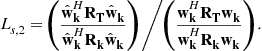
2.12.2.4.1 Clairvoyant SINR loss
Clairvoyant SINR loss is the ratio of output SINR for a filter implementation, ![]() , where all parameters are known precisely, to the maximum SNR. Clairvoyant SINR is given as
, where all parameters are known precisely, to the maximum SNR. Clairvoyant SINR is given as
 (12.51)
A few cases are worth considering:
Case 1—Noise-Limited Condition: In this case, ![]() , where
, where ![]() is the noise power. Then, the maximum SINR weight vector,
is the noise power. Then, the maximum SINR weight vector,
![]() (12.52)
(12.52)
and so
 (12.53)
As expected, the optimal weighting defaults to the matched filter and there is no loss relative to the bound defined by the uncorrelated noise.
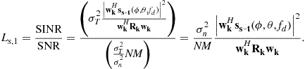
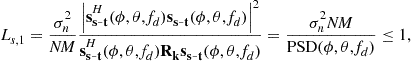
Case 2—Color-Limited Condition, Matched Filter Weights: Clairvoyant loss characterizes the impact of interference on detection performance. Consider the case where the weight vector is set to the space-time matched filter, ![]() . The clairvoyant SINR loss follows from (12.51) as
. The clairvoyant SINR loss follows from (12.51) as
 (12.54)
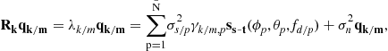
where ![]() is the power spectral density (PSD), equal to the two-dimensional Fourier transform of the space-time covariance matrix [12]; Figure 12.1 provides example clutter-plus-noise PSD plots. Equation (12.54) shows the impact of interference on performance relative to the noise-limited case. Since the PSD is diffraction-limited (the mainlobe is determined by the size of the space-time aperture), (12.54) characterizes the performance impacts of using the deterministic matched filter. At those angles and Doppler frequencies away from the clutter angle-Doppler region of support, the clairvoyant SINR loss approaches the noise-limited case.
is the power spectral density (PSD), equal to the two-dimensional Fourier transform of the space-time covariance matrix [12]; Figure 12.1 provides example clutter-plus-noise PSD plots. Equation (12.54) shows the impact of interference on performance relative to the noise-limited case. Since the PSD is diffraction-limited (the mainlobe is determined by the size of the space-time aperture), (12.54) characterizes the performance impacts of using the deterministic matched filter. At those angles and Doppler frequencies away from the clutter angle-Doppler region of support, the clairvoyant SINR loss approaches the noise-limited case.
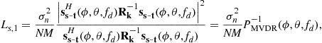
Case 3—Color-Limited Condition, Optimal Weights: Using the maximum SINR weight vector, ![]() , in (12.51), gives
, in (12.51), gives
 (12.55)
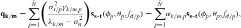
where ![]() is a sample of the MVDR spectrum given in (12.18). Considering the MVDR plots in Figure 12.1, (12.55) suggests regions of loss confined to the sharp, super-resolution contours of the clutter MVDR response (note the inverse in (12.55)). For this reason, STAP is able to detect targets in close proximity to the center of the clutter angle-Doppler region of support. In contrast, (12.54) suggests that SINR loss extends to the full width of the diffraction-limited spectrum when using nonadaptive weights. Figure 12.25, given in Section 2.12.5.3, compares SINR loss for adaptive and nonadaptive solutions, confirming these observations.
is a sample of the MVDR spectrum given in (12.18). Considering the MVDR plots in Figure 12.1, (12.55) suggests regions of loss confined to the sharp, super-resolution contours of the clutter MVDR response (note the inverse in (12.55)). For this reason, STAP is able to detect targets in close proximity to the center of the clutter angle-Doppler region of support. In contrast, (12.54) suggests that SINR loss extends to the full width of the diffraction-limited spectrum when using nonadaptive weights. Figure 12.25, given in Section 2.12.5.3, compares SINR loss for adaptive and nonadaptive solutions, confirming these observations.
2.12.2.4.2 Adaptive SINR loss
Adaptive SINR loss is the ratio of the output SINR for the filter using estimated quantities, ![]() , to the optimal filter output,
, to the optimal filter output, ![]() , where all parameters are clairvoyantly known, viz.
, where all parameters are clairvoyantly known, viz.
 (12.56)
Observe that when ![]() . Moreover,
. Moreover, ![]() , since
, since ![]() yields the maximum output SINR and so the denominator in (12.56) will always be greater than or equal to the numerator.
yields the maximum output SINR and so the denominator in (12.56) will always be greater than or equal to the numerator.
Substituting (12.43) and (12.44) into (12.56) yields
![]() (12.57)
(12.57)
where ![]() is given by (12.7). Assuming
is given by (12.7). Assuming ![]() uses (12.49) in its calculation, as (12.57) suggests, then determining
uses (12.49) in its calculation, as (12.57) suggests, then determining ![]() is critical. This important matter was addressed in [17], where it is shown that (12.57) is Beta distributed, with mean value
is critical. This important matter was addressed in [17], where it is shown that (12.57) is Beta distributed, with mean value
![]() (12.58)
(12.58)
Setting (12.58) equal to ![]() (or, 3 dB of loss) and solving for
(or, 3 dB of loss) and solving for ![]() yields
yields
![]() (12.59)
(12.59)
It is popular to refer to the result in (12.59), where setting ![]() roughly equal to twice the processor’s DoFs yields 3 dB of loss, as the Reed-Mallett-Brennan (RMB) rule after its originators. In practice, 3 dB of loss is substantial, and so choosing
roughly equal to twice the processor’s DoFs yields 3 dB of loss, as the Reed-Mallett-Brennan (RMB) rule after its originators. In practice, 3 dB of loss is substantial, and so choosing ![]() to be at least five times the processor’s DoF is desirable.
to be at least five times the processor’s DoF is desirable.
The IID assumption inherent in the calculation of (12.57) sets the bound on performance for the adaptive processor given ![]() homogeneous training samples. We address the impact of non-IID clutter conditions in further detail in Section 2.12.5.
homogeneous training samples. We address the impact of non-IID clutter conditions in further detail in Section 2.12.5.
2.12.2.4.3 Improvement factor
Improvement factor (IF) is given as the ratio of the output SINR to the input (element-level) SINR [18,19]. IF is given as
 (12.60)
where ![]() is the input (element-level) interference power.
is the input (element-level) interference power.
Case 1—Noise-Limited Condition: In the noise-limited case, ![]() and
and ![]() , and considering the matched filter,
, and considering the matched filter, ![]() , then
, then
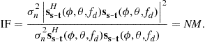 (12.61)
As expected, the improvement factor equals the space-time integration gain in this instance.
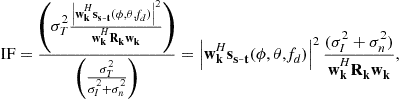
Case 2—Clutter-Limited Condition, Matched Filter Weights: In the clutter-limited case, with ![]() , the improvement factor is
, the improvement factor is
![]() (12.62)
(12.62)
The presence of interference in the PSD degrades the improvement factor. If we let ![]() and
and ![]() in (12.62), we arrive at (12.61).
in (12.62), we arrive at (12.61).
Case 3—Clutter-Limited Condition, Optimal Weights: Using the maximum SINR weight vector, ![]() , in (12.60), gives
, in (12.60), gives
 (12.63)
This expression indicates reduced improvement for those angle-Doppler locations aligning with the clutter, and otherwise good performance in proximity to the clutter response owing to the super-resolution characteristic of ![]() (see Figure 12.1).
(see Figure 12.1).
2.12.2.4.4 Optimal and adaptive filter patterns
The filter gain pattern follows directly by evaluating the filter response over the angles (or spatial frequencies) and Doppler frequencies of interest. Define the space-time steering matrix,
![]() (12.64)
(12.64)
for all ![]() , and
, and ![]() . The optimal gain pattern is
. The optimal gain pattern is
![]() (12.65)
(12.65)
where ![]() is the optimal weighting given by (12.43). The adaptive gain pattern follows similarly as
is the optimal weighting given by (12.43). The adaptive gain pattern follows similarly as
![]() (12.66)
(12.66)
with (12.44) yielding ![]() .
.
Example gain patterns corresponding to the clutter environments shown in Figure 12.1 are given in Figure 12.2. This gain pattern corresponds to (12.65).
2.12.3 Signal models
In this section we consider basic space-time signal and covariance models.
2.12.3.1 Clutter
A plethora of reflected signals from the Earth’s surface comprise what is known as radar ground clutter. Ground clutter is a primary impediment to the detection of moving targets. The clutter signal is predominantly made up of signal reflections from distributed objects, such as returns from soil, forests, fields, etc. Discrete clutter sources are less frequently occurring and spatially distributed with a particular density as a function of RCS, leading to strong, point-like returns. Since clutter discrete returns occur relatively infrequently, their suppression is more challenging and they tend to drive false alarm rate. Many discrete returns result from manmade objects, like buildings, water towers, utility poles, etc. Fence lines, train tracks, and power lines are examples of extended sources of discrete clutter.
We discuss basic distributed and discrete clutter models.
2.12.3.1.1 Distributed clutter
Distributed clutter returns result from the integrated response of all scatterers within the range resolution cell. A model for distributed clutter involves discretizing the range resolution cell into fine angle bins called clutter patches. The location of the angle bin relative to the platform velocity vector determines the clutter patch Doppler frequency. The clutter snapshot then follows as the sum of the returns from each of the individual patches.
Figure 12.6 depicts the discretized clutter patch model for distributed clutter. The antenna gain varies around the range resolution annulus on the Earth’s surface in accordance with the array normal and steering direction. It is common to model the clutter complex voltage as a Gaussian random variable due to the constructive and destructive sum of the returns from the sub-scatterers comprising each resolution cell. The patch clutter-to-noise ratio (CNR) at the channel-level (assuming matched channels) is
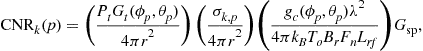 (12.67)
where ![]() is the transmit power,
is the transmit power, ![]() is the transmit gain in the pth direction of interest, r is the slant range,
is the transmit gain in the pth direction of interest, r is the slant range, ![]() is the pth clutter patch radar cross section,
is the pth clutter patch radar cross section, ![]() is the receive channel gain,
is the receive channel gain, ![]() is the center wavelength,
is the center wavelength, ![]() is Boltzman’s constant,
is Boltzman’s constant, ![]() is standard operating temperature,
is standard operating temperature, ![]() is the receiver bandwidth,
is the receiver bandwidth, ![]() is noise figure,
is noise figure, ![]() is RF system loss, and
is RF system loss, and ![]() is signal processing gain (the pulse compression ratio, in this case) [1,7,8]. The clutter RCS is a function of the patch reflectivity,
is signal processing gain (the pulse compression ratio, in this case) [1,7,8]. The clutter RCS is a function of the patch reflectivity, ![]() , and area,
, and area, ![]() , where the area is determined to be a fraction of the resolution cell,
, where the area is determined to be a fraction of the resolution cell,
![]() (12.68)
(12.68)
The constant gamma model is a common choice used to model reflectivity and is given as ![]() , where
, where ![]() is a normalized reflectivity term dependent on the terrain type and
is a normalized reflectivity term dependent on the terrain type and ![]() is the grazing angle to the clutter patch [20]. The clutter patch power then follows by multiplying (12.67) by the receiver noise,
is the grazing angle to the clutter patch [20]. The clutter patch power then follows by multiplying (12.67) by the receiver noise, ![]() . The clutter voltage for the kth range bin and pth patch voltage is then
. The clutter voltage for the kth range bin and pth patch voltage is then
![]() (12.69)
(12.69)
where ![]() [9–11,18,19]. (If the response is non-fluctuating, as in the case of a clutter discrete subsequently discussed, then
[9–11,18,19]. (If the response is non-fluctuating, as in the case of a clutter discrete subsequently discussed, then ![]() is a complex scalar with unity magnitude and uniformly distributed phase.)
is a complex scalar with unity magnitude and uniformly distributed phase.)
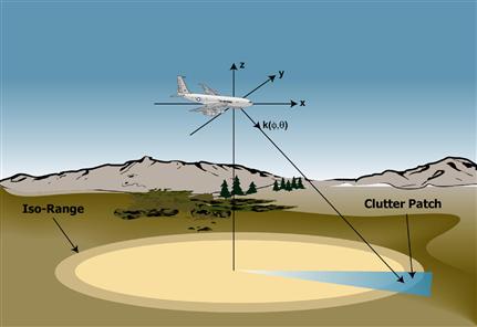
Figure 12.6 Illustration of space-time clutter patch calculation (after [9]). © 2003 IEEE
The patch voltage in (12.69) varies over the space-time aperture: there is a phase change from channel-to-channel due to direction of arrival, described by the spatial steering vector; and, a phase change from pulse-to-pulse due to the change in range-rate between the clutter patch and the radar platform, described by the temporal steering vector. The clutter space-time snapshot then follows by summing the voltages over the P patches for each of Q range ambiguities, where ![]() is the first (unambiguous) range return
is the first (unambiguous) range return
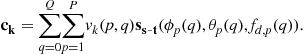 (12.70)
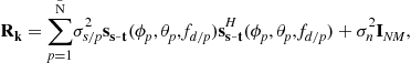
It is common to assume each patch is statistically independent, in which case the clutter covariance matrix corresponding to (12.70) is
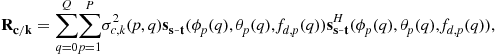 (12.71)
where ![]() is the clutter patch power and follows from (12.69). Equations (12.70) and (12.71) form the basic ground clutter models.
is the clutter patch power and follows from (12.69). Equations (12.70) and (12.71) form the basic ground clutter models.
The clutter voltage decorrelates, mainly in time due to intrinsic clutter motion (ICM). Windswept vegetation and moving water are two cases where ICM results. The two basic models describing clutter temporal decorrelation include the Billingsley model [21] and the Gaussian model [7,10]. The Billingsley model is most common for overland surveillance; it allows a certain amount of the clutter power to decorrelate, say due to leaves fluctuating in the breeze, whilst some of the clutter power is persistent, thus modeling the tree trunk, for example. The Billingsley model leads to an exponential autocorrelation function. In contrast, the Gaussian power spectrum of [7] leads to a Gaussian autocorrelation; the Gaussian model leads to complete decorrelation over a specified time interval and is most appropriate in marine or riverine environments. Dispersion (group delay) across the array is the common source of spatial decorrelation; a sinc autocorrelation model is commonly chosen to model this effect, since it is the inverse transform of a rectangular function in the frequency domain [22,23].
Given the aforementioned discussion, define the length-NM space-time correlation taper as ![]() , with correlation matrix
, with correlation matrix ![]() .
. ![]() is the temporal correlation matrix and
is the temporal correlation matrix and ![]() is the spatial correlation matrix. The resulting clutter covariance matrix is
is the spatial correlation matrix. The resulting clutter covariance matrix is
 (12.72)
Generating space-time clutter snapshots exhibiting the correlation described by ![]() typically involves shaping white noise by multiplying the matrix square root of
typically involves shaping white noise by multiplying the matrix square root of ![]() and
and ![]() by random vectors of length N or M, where the elements of each vector are uncorrelated, zero mean, unity variance Gaussian variates.
by random vectors of length N or M, where the elements of each vector are uncorrelated, zero mean, unity variance Gaussian variates.
2.12.3.1.2 Discrete clutter
Clutter discretes are strong returns that occur relatively infrequently and correspond to stationary, point-like objects, such as parked vehicles, utility poles, water towers, etc. Generally, the RCS of the clutter discrete is large relative to the RCS of a typical, resolved clutter patch. In some cases, the discrete clutter can appear extended, such as in the case of a fence line or train track.
Figure 12.7 shows an example of discrete-like returns in a spotlight synthetic aperture radar (SAR) image of the Mojave Desert Airport. The hangar edges and fence lines, as well as some aircraft on the tarmac, are evident in the figure. Figure 12.8 shows an exceedance plot characterizing the typical impact of clutter discretes on detection performance. (EFA is a post-Doppler STAP method described in Section 2.12.4 and AMF refers to a STAP normalization discussed in Section 2.12.7.) In a homogeneous environment, the output of the STAP is well-behaved and the cumulative distribution follows the expected exponentially-shaped exceedance; in contrast, with discretes present, the tails of the exceedance plot are extended, indicating a requirement to raise the detection threshold to maintain a constant false alarm rate.
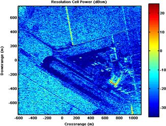
Figure 12.7 Spotlight SAR image of Mojave Desert Airport at 1 m resolution ([24]). © 2004 IEEE

A plausible discrete model involves laying out the spatial locations of discrete clutter of varying densities. One way to do this is to specify the density per km2 for a particular discrete RCS and employ a Poisson distribution to identify the random clutter discrete locations. An example of a range-angle seeding of discrete clutter of varying RCS from 20 dBsm to 60 dBsm is show in Figure 12.9.

Since discrete clutter is stationary, the angular position uniquely specifies Doppler frequency. In other words, clutter discretes reside along the angle-Doppler region of support corresponding to stationary objects. As in the case of distributed clutter, the discrete-to-noise ratio (DNR) follows in a form similar to (12.67) for the lth discrete at range, ![]() , and angle
, and angle ![]() , as
, as
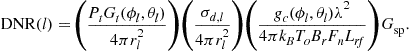 (12.73)
As the discrete is considered point-like, the RCS is taken as nonfluctuating, whereas the phase is uniformly distributed. The corresponding discrete space-time snapshot is
![]() (12.74)
(12.74)
where u is a uniformly-distributed random variable between ![]() and
and ![]() is the range realization for the lth clutter discrete. The discrete clutter is additive. The corresponding covariance matrix for each discrete is
is the range realization for the lth clutter discrete. The discrete clutter is additive. The corresponding covariance matrix for each discrete is
![]() (12.75)
(12.75)
2.12.3.2 Radio frequency interference
Typically, RFI appears as a noise-like, in-band signal source. The RFI can be intentional or not. In the narrowband case, the kth spatial snapshot for the ith RFI source and nth pulse is
![]() (12.76)
(12.76)
where ![]() is an uncorrelated source and T is the PRI. The waveform,
is an uncorrelated source and T is the PRI. The waveform, ![]() , is generally uncorrelated at nonzero lags, viz.,
, is generally uncorrelated at nonzero lags, viz.,
![]() (12.77)
(12.77)
but otherwise fully correlated for very short time lags corresponding to propagation across the multi-channel array, as (12.76) indicates (thus, ![]() , for
, for ![]() , in the narrowband case). The corresponding spatial covariance matrix is
, in the narrowband case). The corresponding spatial covariance matrix is
![]() (12.78)
(12.78)
As a result of (12.77), the space-time covariance matrix is
 (12.79)
Thus, a spatial null is sufficient to remove the narrow-band RFI, as no temporal correlation is present.
Each RFI source is considered statistically independent, so that for J sources, ![]() , where
, where ![]() is the space-time snapshot and
is the space-time snapshot and ![]() .
.
As the fractional bandwidth—the ratio of waveform bandwidth to center frequency—of the receive signal increases, dispersion occurs. Dispersion leads to decorrelation of the RFI over the receive array; in this case, a single RFI signal appears as multiple, closely spaced sources in angle [23]. In general, the wideband RFI suppression case is handled similar to the narrowband case through the use of subband filtering or the use of fast-time taps. In the former case, the subbanding is commonly implemented using polyphase filtering, allowing the processor to implement the narrowband canceler in each subband prior to recombining [25].
2.12.3.3 Receiver noise
Uncorrelated noise sources—such as receiver noise or sky noise—are modeled as a white Gaussian noise (WGN) disturbance, ![]() , where m and n are channel and pulse indices, respectively, and
, where m and n are channel and pulse indices, respectively, and ![]() . The waveform samples are assumed uncorrelated such that
. The waveform samples are assumed uncorrelated such that
![]() (12.80)
(12.80)
where ![]() is the channel noise power. This noise source is also uncorrelated, independent, and identically distributed over the range dimension.
is the channel noise power. This noise source is also uncorrelated, independent, and identically distributed over the range dimension.
2.12.3.4 Target
The target snapshot is generally modeled using both Swerling 1 and Swerling 2 statistics [1,7,8]. Swerling 1 and Swerling 2 targets each exhibit voltages corresponding to a circular Gaussian distribution; the Gaussian nature of the voltage distribution models target fading effects. The target voltage is assumed perfectly correlated within the CPI, in accord with the Swerling 1 model, and uncorrelated from CPI-to-CPI according to the Swerling 2 target model. Frequency hopping from CPI-to-CPI is a common reason for target voltage decorrelation and is used to minimize the impact of target fading on detection performance. STAP is applied on a CPI basis, as it is a coherent signal processing technique, with noncoherent addition (NCA) applied to the STAP output—from CPI-to-CPI—to mitigate target fading effects.
Using the Swerling 1 target model, the target snapshot at the kth range, Doppler frequency, ![]() , and angle,
, and angle, ![]() , is
, is
![]() (12.81)
(12.81)
where ![]() and SNR is the single channel, single pulse signal-to-noise ratio. The random variable,
and SNR is the single channel, single pulse signal-to-noise ratio. The random variable, ![]() , models targeting fading resulting from subscatterers adding in and out of phase. As indicated, to handle fading, it is common to frequency hop from CPI-to-CPI, in which case target voltages appear decorrelated (Swerling 2).
, models targeting fading resulting from subscatterers adding in and out of phase. As indicated, to handle fading, it is common to frequency hop from CPI-to-CPI, in which case target voltages appear decorrelated (Swerling 2).
Nonfluctuating, point-target analysis employs (12.81) with ![]() , where u is uniformly distributed between
, where u is uniformly distributed between ![]() . Sometimes the nonfluctuating target model is used in analysis. However, the Swerling 2 model is the preferred choice, with the Swerling 1 model applicable at the fixed frequency, CPI-level.
. Sometimes the nonfluctuating target model is used in analysis. However, the Swerling 2 model is the preferred choice, with the Swerling 1 model applicable at the fixed frequency, CPI-level.
2.12.3.5 The space-time snapshot
The space-time snapshot for realization, k, is given by (12.2) with the addition of clutter discretes, where the possibility of the single target case is
 (12.82)
where D is the total number of discrete scatterers and the snapshot terms, ![]() , are only added when
, are only added when ![]() . The null-hypothesis covariance matrix corresponding to (12.82) is
. The null-hypothesis covariance matrix corresponding to (12.82) is
 (12.83)
where, as expected, ![]() is included only for those terms where
is included only for those terms where ![]() .
.
It is common to envision the collection of space-time snapshots organized as space-time data matrices,
![]() (12.84)
(12.84)
The spatial snapshot for pulse, n, is denoted as ![]() ; it results by removing N length-M segments from
; it results by removing N length-M segments from ![]() and stacking them side-by-side. The pictorial of (12.84) is given in Figure 12.10 and is known as the radar datacube. Generally, the STAP operates on each space-time data matrix, or slice, of the cube in Figure 12.10, while using slices at other ranges (or realizations) for training. We subsequently describe various adaptive implementations. (Note: space/fast-time processing uses slices along the pulse/fast-time domain and can train over the pulse dimension. As previously mentioned, we focus on space/slow-time adaptivity, but the basic formulations of the next section generally apply to any appropriately formatted data with the corresponding restrictions of each method.)
and stacking them side-by-side. The pictorial of (12.84) is given in Figure 12.10 and is known as the radar datacube. Generally, the STAP operates on each space-time data matrix, or slice, of the cube in Figure 12.10, while using slices at other ranges (or realizations) for training. We subsequently describe various adaptive implementations. (Note: space/fast-time processing uses slices along the pulse/fast-time domain and can train over the pulse dimension. As previously mentioned, we focus on space/slow-time adaptivity, but the basic formulations of the next section generally apply to any appropriately formatted data with the corresponding restrictions of each method.)

Figure 12.10 Radar datacube (after [9]). © 2003 IEEE
2.12.4 Adaptive filter implementations
Section 2.12.2.2 describes space-time filter formulations. As seen from the discussion, all solutions are similar, involving space-time weightings of the form of a covariance inverse and a steering vector to implement the matched filter.
We now discuss three basic paradigms to implement the weighting strategies discussed in Section 2.12.2.2: reduced-rank STAP (RR-STAP), reduced-dimension STAP (RD-STAP), and parametric STAP.
2.12.4.1 Reduced-rank STAP
As seen from (12.78), each narrowband RFI source is rank-one. Distributed clutter is oftentimes of rank significantly less than the dimensionality of ![]() , viz.
, viz. ![]() . Through empirical analysis, the clutter rank for a sidelooking radar with minimal yaw is approximated as
. Through empirical analysis, the clutter rank for a sidelooking radar with minimal yaw is approximated as
![]() (12.85)
(12.85)
where ![]() is the platform along-track velocity and d is the separation between channels of a uniform linear array (ULA) [10]. The expression in (12.85) is known as Brennan’s Rule; a related rule is given by Klemm [26]. Brennan’s rule is closely related to the number of independent antenna channel positions during the collection interval; redundancy in the measurements lowers the rank, and in fact leads to coloration of the clutter return. The idea behind RR-STAP is to essentially project the interference subspace—those eigenspaces corresponding to larger eigenvalues above the noise floor—out of the space-time snapshot.
is the platform along-track velocity and d is the separation between channels of a uniform linear array (ULA) [10]. The expression in (12.85) is known as Brennan’s Rule; a related rule is given by Klemm [26]. Brennan’s rule is closely related to the number of independent antenna channel positions during the collection interval; redundancy in the measurements lowers the rank, and in fact leads to coloration of the clutter return. The idea behind RR-STAP is to essentially project the interference subspace—those eigenspaces corresponding to larger eigenvalues above the noise floor—out of the space-time snapshot.
The eigendecomposition of the space-time covariance matrix yields
 (12.86)
where ![]() is the mth eigenvalue corresponding to eigenvector
is the mth eigenvalue corresponding to eigenvector ![]() ,
, ![]() represents the interference subspace eigenvalues, and
represents the interference subspace eigenvalues, and ![]() characterizes the noise subspace eigenvalues. The interference eigenvectors have the special property that each span the collection of interference steering vectors. Moreover,
characterizes the noise subspace eigenvalues. The interference eigenvectors have the special property that each span the collection of interference steering vectors. Moreover, ![]() is unitary, so
is unitary, so
![]() (12.87)
(12.87)
We can write the distributed clutter-plus-noise part of (12.83) in a generic, simplified form
 (12.88)
where ![]() is the number of signal sources and
is the number of signal sources and ![]() is the power for the pth signal source. While this simplified covariance form suggests a model for clutter-plus-noise, the subsequent results are extensible to other correlated sources. Then, from (12.88),
is the power for the pth signal source. While this simplified covariance form suggests a model for clutter-plus-noise, the subsequent results are extensible to other correlated sources. Then, from (12.88),
 (12.89)
where
![]() (12.90)
(12.90)
Solving (12.89) for the mth eigenvector, ![]() ,
,
 (12.91)
where in this case
 (12.92)
Naturally, these equations are only valid for the dominant subspace, ![]() . Equation (12.91) shows
. Equation (12.91) shows ![]() .
.
Also, it is known that any wide-sense stationary (WSS) process with zero mean and covariance matrix, ![]() , can be written as a linear combination of the eigenvectors of
, can be written as a linear combination of the eigenvectors of ![]() , via what is known as the Karhunen-Loève Transform (KLT),
, via what is known as the Karhunen-Loève Transform (KLT),
 (12.93)
where ![]() are the Karhunen- Loève (KL) coefficients [12].
are the Karhunen- Loève (KL) coefficients [12].
The prior expressions, (12.86)–(12.93), provide necessary mathematical background for our subsequent discussion on RR-STAP methods.
Motivation for RR-STAP includes the following:
• Clutter and jamming tend to be of low numerical rank and the processor explicitly removes only those signal subspaces corresponding to interference.
• The eigendecomposition maximally compresses the interference into the fewest basis vectors [12].
• The RMB rule applies to the RR-STAP case, with rank replacing DoFs in the formulation, viz. training over twice the rank yields roughly 3 dB loss on average [27].
In effect, RR-STAP is a weight calculation strategy. There are challenges implementing RR-STAP, including high computational burden and difficulties in rank determination. Nevertheless, RR-STAP methods hold meaningful insight and, in some cases, are useful in weight vector determination.
2.12.4.1.1 Adaptive beamformer pattern synthesis
It is shown in [28] that (12.43) can be written
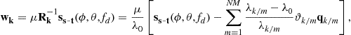 (12.94)
where ![]() is the noise-floor eigenvalue level and
is the noise-floor eigenvalue level and ![]() is the projection of the mth eigenvector onto the quiescent pattern. As seen from (12.94), the STAP response appears as a notching of the space-time beampattern given by
is the projection of the mth eigenvector onto the quiescent pattern. As seen from (12.94), the STAP response appears as a notching of the space-time beampattern given by ![]() by the weighted, interference eigenvectors. When
by the weighted, interference eigenvectors. When ![]() , no subtraction occurs, since the corresponding eigenvector lies in the noise subspace.
, no subtraction occurs, since the corresponding eigenvector lies in the noise subspace.
Naturally, (12.94) applies to the SMI formulation of (12.44), and can provide robustness in the presence of training sample support limitations if the interference rank is known (which is usually only practical for strong interferers). Specifically, running the sum in (12.94) only over ![]() subspaces leads to adaptive pattern robustness, since low sample support tends to predominantly perturb the noise subspace; the perturbed noise subspace estimate leads to poor adaptive sidelobe performance when the sum in (12.94) is run over all values of the index, m.
subspaces leads to adaptive pattern robustness, since low sample support tends to predominantly perturb the noise subspace; the perturbed noise subspace estimate leads to poor adaptive sidelobe performance when the sum in (12.94) is run over all values of the index, m.
2.12.4.1.2 Principle components inverse
The idea behind principle components inverse (PCI) is to apply an orthogonal projection to ![]() , and then apply a matched filter to the remaining transformed data [29]. The PCI formulation starts by writing (12.94) applied to the data as
, and then apply a matched filter to the remaining transformed data [29]. The PCI formulation starts by writing (12.94) applied to the data as
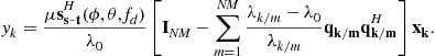 (12.95)
Then, for the ![]() eigenvalues where
eigenvalues where ![]() ,
,
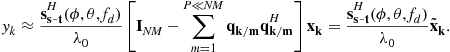 (12.96)
 (12.97)
where, for the case of ![]() as an example, (12.97) shows the coherent removal of
as an example, (12.97) shows the coherent removal of ![]() and
and ![]() . The term in brackets in (12.97) is called an orthogonal projection for this reason.
. The term in brackets in (12.97) is called an orthogonal projection for this reason.
2.12.4.1.3 Eigencanceler
Haimovich [30] gives two different developments; one of these essentially leads to (12.96) via an alternate route.
The minimum power eigencanceler (MPE) weighting results from
![]() (12.98)
(12.98)
where ![]() is a constraint matrix and
is a constraint matrix and ![]() is a desired response vector. The solution to (12.98) is shown in [30] to be
is a desired response vector. The solution to (12.98) is shown in [30] to be
![]() (12.99)
(12.99)
For the case where ![]() and
and ![]() , (12.99) takes the form
, (12.99) takes the form
![]() (12.100)
(12.100)
with ![]() a scalar. The weight vector in (12.100) lies entirely in the noise subspace—as required by (12.98)—and will, by virtue of the orthonormal property of the set of eigenvectors, annihilate the clutter subspace.
a scalar. The weight vector in (12.100) lies entirely in the noise subspace—as required by (12.98)—and will, by virtue of the orthonormal property of the set of eigenvectors, annihilate the clutter subspace.
The minimum norm eigencanceler (MNE) is formulated as
![]() (12.101)
(12.101)
The MNE weight vector is then shown in [30] to be
![]() (12.102)
(12.102)
Again, for the case where ![]() and
and ![]() , and using (12.87), we see (12.102) can be written in the same form as PCI,
, and using (12.87), we see (12.102) can be written in the same form as PCI,
![]() (12.103)
(12.103)
with ![]() a scaling that replaces
a scaling that replaces ![]() in (12.96). Using (12.87), the expression in (12.103) can be written
in (12.96). Using (12.87), the expression in (12.103) can be written
![]() (12.104)
(12.104)
which closely relates to the MPE solution in (12.100) with the inverse eigenvalue weighting given by ![]() absent. It is known that limited training sample support leads to perturbed estimates of the noise eigenvalues appearing along the diagonal of
absent. It is known that limited training sample support leads to perturbed estimates of the noise eigenvalues appearing along the diagonal of ![]() . For this reason, the MNE provides robustness relative to MPE when training data samples are lacking.
. For this reason, the MNE provides robustness relative to MPE when training data samples are lacking.
2.12.4.1.4 Hung turner projection
The Hung Turner Projection (HTP) is applicable to RFI suppression [31]. While clutter mitigation is paramount to our discussion, it is worth taking a moment to describe the HTP as a general tool in adaptive filter implementation. Reducing computational burden associated with the eigendecomposition leading to the eigenvalues and eigenvectors of the null-hypothesis covariance matrix is a primary goal.
The basic idea behind the HTP is to use the Gram-Schmidt method to characterize the interference subspace. Specifically, suppose we identify J snapshots where J RFI sources are present,
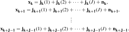 (12.105)
Next, the modified Gram-Schmidt technique is applied to (12.105) to generate the orthonormal basis, ![]() , where
, where ![]() . Then, in accord with [31], the HTP weight vector is chosen as
. Then, in accord with [31], the HTP weight vector is chosen as ![]() , with
, with
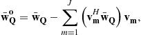 (12.106)
and where ![]() is the quiescent weight vector.
is the quiescent weight vector.
2.12.4.1.5 Diagonal loading
Diagonal loading involves adding a scaled diagonal matrix to the covariance matrix estimate of (12.49) [32],
 (12.107)
where ![]() is the diagonal loading level and
is the diagonal loading level and ![]() and
and ![]() follow from the decomposition of the covariance matrix estimate. It is common to set
follow from the decomposition of the covariance matrix estimate. It is common to set ![]() , with
, with ![]() most typical. Primary benefits of diagonal loading include improved conditioning of the covariance matrix estimate (which improves the numerical stability of inversion routines) and compression of the range corresponding to the smallest eigenvalues. This latter benefit leads to a reduction in spurious sidelobes of the adapted pattern at the expense of null depth. Effectively, diagonal loading removes some of the adaptivity of the system to better condition the filter’s sidelobe response.
most typical. Primary benefits of diagonal loading include improved conditioning of the covariance matrix estimate (which improves the numerical stability of inversion routines) and compression of the range corresponding to the smallest eigenvalues. This latter benefit leads to a reduction in spurious sidelobes of the adapted pattern at the expense of null depth. Effectively, diagonal loading removes some of the adaptivity of the system to better condition the filter’s sidelobe response.
While often considered ad hoc, it turns out diagonal loading is a component of the optimal solution to the constrained optimization,
![]() (12.108)
(12.108)
The Lagrangian for (12.108) is readily found to be
![]() (12.109)
(12.109)
where ![]() and
and ![]() are Lagrangian multipliers. Taking the gradient of (12.109) with respect to the conjugate of the weight vector and setting the result to zero yields [13]
are Lagrangian multipliers. Taking the gradient of (12.109) with respect to the conjugate of the weight vector and setting the result to zero yields [13]
![]() (12.110)
(12.110)
Solving for the weight vector gives
![]() (12.111)
(12.111)
Using the linear constraint, it is seen that
![]() (12.112)
(12.112)
The resulting weight vector is
 (12.113)
From (12.113) we see that diagonal loading plays a key role in the solution to the constrained optimization. In this case, ![]() is the diagonal loading level,
is the diagonal loading level, ![]() , mentioned previously. If the loading level is set to zero, (12.113) defaults to the distortionless MV beamformer solution.
, mentioned previously. If the loading level is set to zero, (12.113) defaults to the distortionless MV beamformer solution.
2.12.4.1.6 Cross spectral metric
Consider the GSLC structure of Figure 12.5. A principal components approximation to ![]() is
is
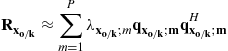 (12.114)
with, ideally, ![]() , and where
, and where ![]() and
and ![]() represent the mth eigenvalue and eigenvector of the GSLC lower leg covariance matrix. Then,
represent the mth eigenvalue and eigenvector of the GSLC lower leg covariance matrix. Then,
 (12.115)
The computational burden of the GSLC does not generally justify its use in practice. Improved statistical convergence is a potential advantage of the principal components decomposition of the GSLC (PC-GSLC).
The cross spectral metric operates in a fashion similar to the PC-GSLC method, except now the selection of the basis defining the rank-reducing transformation is target signal-dependent [33]. The error signal at the output of the GSLC follows as the difference between (12.19) and (12.21), viz.
![]() (12.116)
(12.116)
The corresponding MMSE is given as the expected value of the magnitude squared of (12.116),
 (12.117)
In this case, ![]() , where no target signal energy is present in the upper leg (an assumption that carries through in the calculation of the cross correlation vector,
, where no target signal energy is present in the upper leg (an assumption that carries through in the calculation of the cross correlation vector, ![]() ). When choosing only P terms in the summation of (12.117), where
). When choosing only P terms in the summation of (12.117), where ![]() , the processor attains the lowest possible mean square error (MSE) by choosing subspaces with the largest cross-spectral metric terms, given as
, the processor attains the lowest possible mean square error (MSE) by choosing subspaces with the largest cross-spectral metric terms, given as
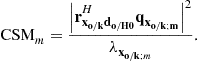 (12.118)
The target signal influences the selection via ![]() . Thus, the idea behind the CSM approach is to select only those subspaces from
. Thus, the idea behind the CSM approach is to select only those subspaces from ![]() that most greatly enhance performance.
that most greatly enhance performance.
A direct-form implementation of the CSM method is given in [34]. In this case, the objective involves maximizing SINR by choosing the appropriate, signal-dependent, reduced-rank subspace (hence, the analogous metric is called the SINR metric in [34]). Thus, decomposing output SINR in (12.7) using the inverse of the eigendecomposition in (12.86) gives
 (12.119)
Maximizing SINR requires choosing the largest terms in (12.119) of the form,
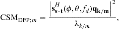 (12.120)
where DFP signifies “direct form processor” (i.e., the approach using a weight vector of the form given in (12.43) or (12.44)). Thus, with limited sample support and uncertainty over the interference rank, selecting the ![]() largest CSM terms of (12.120) leads to maximal output SINR. Commonly, then, the CSM-DFP chooses the components in the noise subspace, but this is an artifact of the development and not useful: terms with the smallest eigenvalues are generally chosen, with any signal-dependent correlation meant to aid in selecting the most significant terms lost in the formulation. To avoid this scenario, [34] suggests choosing those terms maximally impacting the weight vector. In other words, considering (12.94), selecting the P largest terms of
largest CSM terms of (12.120) leads to maximal output SINR. Commonly, then, the CSM-DFP chooses the components in the noise subspace, but this is an artifact of the development and not useful: terms with the smallest eigenvalues are generally chosen, with any signal-dependent correlation meant to aid in selecting the most significant terms lost in the formulation. To avoid this scenario, [34] suggests choosing those terms maximally impacting the weight vector. In other words, considering (12.94), selecting the P largest terms of
![]() (12.121)
(12.121)
most greatly impacts the adaptive process. Equation (12.121) is signal-dependent and forces the selection to lie in the dominant subspace.
2.12.4.1.7 Multi-Stage Wiener Filter
The Multi-Stage Wiener Filter (MWF) is a truncated decomposition of the GSLC of Figure 12.5 [35]. Its operation is best understood from the diagram in Figure 12.11, which shows a two-stage decomposition. From this figure we see that the estimation stage is broken into a series of smaller problems, where the weight vector is calculated as a scalar using the Wiener-Hopf equation [12,13] in each stage. The filter, ![]() , is a normalized cross-correlation vector between its input,
, is a normalized cross-correlation vector between its input, ![]() , and the output of the filter in the preceding leg,
, and the output of the filter in the preceding leg, ![]() ; the intent of choosing
; the intent of choosing ![]() in this manner is to maximize the correlation between the interference signal in each leg. Specifically,
in this manner is to maximize the correlation between the interference signal in each leg. Specifically,
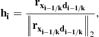 (12.122)
where ![]() . The blocking matrix,
. The blocking matrix, ![]() , lies in the null space of
, lies in the null space of ![]() (expect for
(expect for ![]() , where
, where ![]() . The weights,
. The weights, ![]() , are scalars equal to the Wiener weight minimizing the mean square error between
, are scalars equal to the Wiener weight minimizing the mean square error between ![]() and
and ![]() . In this figure, for the MWF output to equal the GSLC output, the processor must calculate all quantities, including the vector weight,
. In this figure, for the MWF output to equal the GSLC output, the processor must calculate all quantities, including the vector weight, ![]() . The MWF truncates the number of stages by simply dropping the lower leg of the last stage, setting the vector weight to all zeros (i.e.,
. The MWF truncates the number of stages by simply dropping the lower leg of the last stage, setting the vector weight to all zeros (i.e., ![]() ) so that
) so that ![]() , where
, where ![]() is the number of MWF stages. So, for
is the number of MWF stages. So, for ![]() .
.
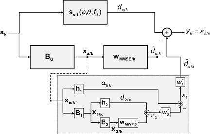
In the adaptive version of the MWF, the processor replaces the known covariance matrices and steering vectors with estimates. The quantities, ![]() , and, naturally,
, and, naturally, ![]() , are all expressible as linear transformations applied to
, are all expressible as linear transformations applied to ![]() and
and ![]() ; in the adaptive filter,
; in the adaptive filter, ![]() and
and ![]() . The implementation requires first calculating and applying
. The implementation requires first calculating and applying ![]() ; next, the processor implements the first stage, calculating
; next, the processor implements the first stage, calculating ![]() , and
, and ![]() ; with these first stage quantities in hand, the processor calculates the second stage quantities,
; with these first stage quantities in hand, the processor calculates the second stage quantities, ![]() , and
, and ![]() , then third stage quantities, and so forth, working out to the last stage; then, as noted above, the error signal in the last stage is set to
, then third stage quantities, and so forth, working out to the last stage; then, as noted above, the error signal in the last stage is set to ![]() , where
, where ![]() is the last stage; and, finally, the scalar weights,
is the last stage; and, finally, the scalar weights, ![]() , are solved from the outer (last) stage into the first stage.
, are solved from the outer (last) stage into the first stage.
While the computational loading of the MWF is generally high, the target signal-dependent nature of the stage decomposition identifies the interference subspace most greatly impacting the MMSE through the cross-correlation process, estimates it, and subtracts it out. This allows the MWF to converge towards the optimal solution with minimal use of available training data.
2.12.4.2 Reduced-dimension STAP
Reduced-dimension STAP (RD-STAP) methods take advantage of the structure of the clutter angle-Doppler region of support to minimize filter length, thus reducing computational burden and training sample requirements. A taxonomy of RD-STAP methods, organized similarly to the discussion in [10], is given in Figure 12.12.

RD-STAP methods apply deterministic, linear filtering operations and dimensionality reduction prior to adaptive filtering. A linear transformation, ![]() , where
, where ![]() is the length of the reduced dimension, describes these deterministic operations. Starting with the space-time snapshot,
is the length of the reduced dimension, describes these deterministic operations. Starting with the space-time snapshot, ![]() , the reduced-dimension snapshot is
, the reduced-dimension snapshot is
![]() (12.123)
(12.123)
Via this transformation, the null-hypothesis covariance matrix is
![]() (12.124)
(12.124)
and the target steering vector becomes
![]() (12.125)
(12.125)
The corresponding optimal weighting follows from (12.43) as
![]() (12.126)
(12.126)
The adaptive weighting usually follows by forming the sample covariance matrix of (12.49) from the reduced-dimension data,
![]() (12.127)
(12.127)
forming its inverse, and using ![]() in place of (12.125), viz.
in place of (12.125), viz.
![]() (12.128)
(12.128)
In this case, ![]() is a scalar that usually depends on estimated quantities.
is a scalar that usually depends on estimated quantities.
Motivations for RD-STAP include the following:
• The clutter exhibits a highly structured angle-Doppler region of support, as shown in Figure 12.13. In this figure, T1 and T2 are target locations and C1–C4 are clutter regions. Target T1 predominantly competes with clutter located at C3, and a spatial null within the corresponding Doppler filter suffices to mitigate clutter. Clutter at other locations—such as at C1, C2, and C4—has no significant bearing on target detection. Alternately, target T2 is impacted by clutter in the region of C1 and C4; a two-dimensional null, positioned in angle and Doppler, is needed to suppress mainlobe and near-in sidelobe clutter.
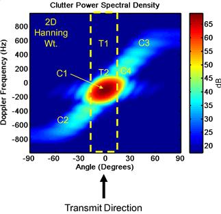
• The RMB rule of Section 2.12.2.4.2 applies to RD-STAP, with ![]() . It is not uncommon to have
. It is not uncommon to have ![]() , whereas
, whereas ![]() is reasonable. Thus, limited and potentially heterogeneous or nonstationary training sample support is reduced by a factor of 10–100 or more.
is reasonable. Thus, limited and potentially heterogeneous or nonstationary training sample support is reduced by a factor of 10–100 or more.
• The implicit inverse of the sample covariance matrix is ![]() , being reduced to
, being reduced to ![]() in the RD-STAP case. For each halving of the processor’s DoFs, computational burden decreases by a factor of eight. Real-time operation requires RD-STAP methods.
in the RD-STAP case. For each halving of the processor’s DoFs, computational burden decreases by a factor of eight. Real-time operation requires RD-STAP methods.
2.12.4.2.1 Post-Doppler STAP
Of the various RD-STAP methods, post-Doppler STAP techniques are most popular. Post-Doppler STAP is shown in the lower left and right of Figure 12.12, where the lower left box corresponds to the so-called “channel space,” post-Doppler methods that operate on space-Doppler data, and the lower right box characterizes the post-Doppler, (spatial) beamspace methods. The Extended Factored Algorithm (EFA) is an example of a “channel space,” post-Doppler method [36]. In EFA, each channel is Doppler filtered, and then the adaptive weighting of (12.128) is applied to the transformed data vector,
![]() (12.129)
(12.129)
where ![]() is the spatial snapshot corresponding to the qth Doppler bin output (i.e., the qth Doppler bin output from channel 1 through M stacked in a vector). Equation (12.129) shows, as an example, the case of five adjacent Doppler bins. The EFA output for the kth range bin and nth Doppler bin is then given by
is the spatial snapshot corresponding to the qth Doppler bin output (i.e., the qth Doppler bin output from channel 1 through M stacked in a vector). Equation (12.129) shows, as an example, the case of five adjacent Doppler bins. The EFA output for the kth range bin and nth Doppler bin is then given by ![]() , where
, where ![]() corresponds to the nth Doppler bin output. Figure 12.14 depicts the EFA processing architecture, where
corresponds to the nth Doppler bin output. Figure 12.14 depicts the EFA processing architecture, where ![]() is the EFA weight applied to the mth channel and qth Doppler bin. This figure shows the case of processing three adjacent Doppler bins; EFA typically employs three or five adjacent bins. The special case of one Doppler bin—where the processor only generates a spatial null—is known as Factored Time-Space (FTS) [10].
is the EFA weight applied to the mth channel and qth Doppler bin. This figure shows the case of processing three adjacent Doppler bins; EFA typically employs three or five adjacent bins. The special case of one Doppler bin—where the processor only generates a spatial null—is known as Factored Time-Space (FTS) [10].

Figure 12.15 describes EFA operation in the angle-Doppler domain. Each horizontal, rectangular box corresponds to a Doppler filter extent. The circles correspond to null locations EFA is able to generate. EFA can generate up to ![]() nulls, where
nulls, where ![]() is the number of temporal DoFs (the number of Doppler bins used in the adaptive combiner). The target location, T1, is shown close to mainlobe clutter. Nulling along the section of the clutter ridge in proximity to T1 is required for target detection. EFA is able to effectively suppress the clutter local to the target position. Its performance benchmarks very close to that of the space-time optimal solution, as will be shown in Section 2.12.5. FTS can generate up to
is the number of temporal DoFs (the number of Doppler bins used in the adaptive combiner). The target location, T1, is shown close to mainlobe clutter. Nulling along the section of the clutter ridge in proximity to T1 is required for target detection. EFA is able to effectively suppress the clutter local to the target position. Its performance benchmarks very close to that of the space-time optimal solution, as will be shown in Section 2.12.5. FTS can generate up to ![]() spatial nulls within the Doppler bin; as seen in this case, given the closeness of T1 to mainlobe clutter, only nulling sidelobe clutter is insufficient.
spatial nulls within the Doppler bin; as seen in this case, given the closeness of T1 to mainlobe clutter, only nulling sidelobe clutter is insufficient.
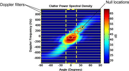
References [37,38] describe post-Doppler, (spatial) beamspace methods. The Joint Domain Localized (JDL) algorithm generalizes EFA by applying a beamspace transformation prior to Doppler filtering in Figure 12.14. JDL then combines ![]() spatial beams and
spatial beams and ![]() Doppler bins to suppress clutter, in a manner similar to a two-dimensional sidelobe canceler. For example, a common configuration is
Doppler bins to suppress clutter, in a manner similar to a two-dimensional sidelobe canceler. For example, a common configuration is ![]() and
and ![]() ; in this three beam configuration, the processor uses the eight angle-Doppler beams surrounding the center beam to estimate and coherently remove the clutter signal in this ninth angle-Doppler direction of interest, thereby exploiting the structure of the clutter local to the target position. JDL performance tends to benchmark well relative to the space-time optimal solution. A special case of JDL is given in [38], where the Doppler filtering is applied to sum and difference beams, and then “auxiliary” beams about the sum beam and Doppler bin of interest are adapted to coherently remove the clutter signal. This latter method has been called Sigma-Delta STAP. Reference [39] also includes germane discussion.
; in this three beam configuration, the processor uses the eight angle-Doppler beams surrounding the center beam to estimate and coherently remove the clutter signal in this ninth angle-Doppler direction of interest, thereby exploiting the structure of the clutter local to the target position. JDL performance tends to benchmark well relative to the space-time optimal solution. A special case of JDL is given in [38], where the Doppler filtering is applied to sum and difference beams, and then “auxiliary” beams about the sum beam and Doppler bin of interest are adapted to coherently remove the clutter signal. This latter method has been called Sigma-Delta STAP. Reference [39] also includes germane discussion.
Additional post-Doppler STAP methods based on PRI designs are given in [10].
2.12.4.2.2 Pre-Doppler STAP
Pre-Doppler STAP—sometimes called adaptive displaced phase center antenna (ADPCA)—involves processing overlapped sub-CPIs to mitigate clutter, then applying Doppler processing to the aggregated output [10,40]. It has particular application in those situations where the clutter response decorrelates during the course of the CPI, such as when the antenna array rotates. Figure 12.16 shows the pre-Doppler STAP, or ADPCA, architecture for the three pulse case.

The corresponding ADPCA data snapshot for three pulses is simply
![]() (12.130)
(12.130)
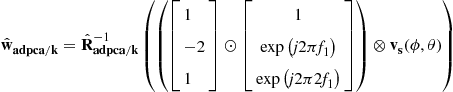 (12.131)
with ![]() the peak clutter Doppler times the PRI. The
the peak clutter Doppler times the PRI. The ![]() -by-
-by-![]() ADPCA covariance matrix estimate,
ADPCA covariance matrix estimate, ![]() , is an approximation to
, is an approximation to
![]() (12.132)
(12.132)
where ![]() is given in (12.130). The covariance inverse in the ADPCA weight vector provides a dynamic response to whiten ground clutter returns. The steering vector term in parentheses suppresses mainlobe clutter with the binominal weights, identified as
is given in (12.130). The covariance inverse in the ADPCA weight vector provides a dynamic response to whiten ground clutter returns. The steering vector term in parentheses suppresses mainlobe clutter with the binominal weights, identified as ![]() , while forming a beam in a specified angular direction; the steering vector incorporates an additional linear phase variation over the temporal pulses to steer the Doppler null in cases where clutter is not centered at 0 Hz.
, while forming a beam in a specified angular direction; the steering vector incorporates an additional linear phase variation over the temporal pulses to steer the Doppler null in cases where clutter is not centered at 0 Hz.
The performance of ADPCA is generally not as good as post-Doppler STAP techniques, thus limiting its use in practice. Performance benchmark results are given in Section 2.12.5.
2.12.4.3 Parametric adaptive matched filter
The parametric adaptive matched filtering (PAMF) employs multichannel, linear prediction to estimate the covariance matrix inverse [41]. We now discuss the PAMF based on [41,42].
Consider the LDU decomposition of the covariance matrix inverse,
![]() (12.133)
(12.133)
where ![]() , and
, and ![]() is diagonal. Since we are considering space-time data, a block LDU decomposition is required. In this case,
is diagonal. Since we are considering space-time data, a block LDU decomposition is required. In this case, ![]() takes the form, for the example of
takes the form, for the example of ![]() and
and ![]() ,
,
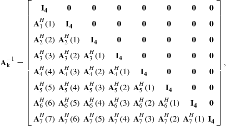 (12.134)
where ![]() are the 4-by-4 multi-channel linear prediction (MCLP) coefficients for the p-order filter and the nth lag,
are the 4-by-4 multi-channel linear prediction (MCLP) coefficients for the p-order filter and the nth lag, ![]() is the 4-by-4 zero matrix, and the realization index, k, is dropped for notational convenience [42]. The matrix
is the 4-by-4 zero matrix, and the realization index, k, is dropped for notational convenience [42]. The matrix ![]() is
is
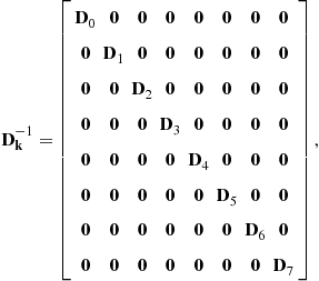 (12.135)
where ![]() is the 4-by-4 inverse of the MCLP error for the p-order filter. As noted in [42], the MCLP development, while not necessary, is useful and provides a framework to calculate
is the 4-by-4 inverse of the MCLP error for the p-order filter. As noted in [42], the MCLP development, while not necessary, is useful and provides a framework to calculate ![]() and
and ![]() .
.
The PAMF uses the LDU decomposition to approximate ![]() . For example, let the maximum MCLP filter order
. For example, let the maximum MCLP filter order ![]() , then
, then
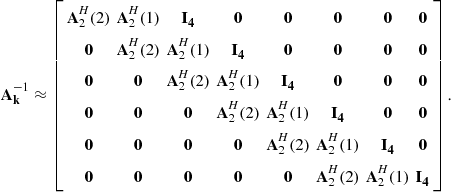 (12.136)
Extending the Wiener-Hopf equation to calculate the linear prediction coefficients, ![]() , and augmenting with the identity matrices shown in (12.136), gives an approximation to
, and augmenting with the identity matrices shown in (12.136), gives an approximation to ![]() . The linear prediction error terms are given as
. The linear prediction error terms are given as
 (12.137)
Generally, each of the diagonal blocks is inverted after solving for ![]() . The approximation to the covariance matrix inverse follows from (12.133).
. The approximation to the covariance matrix inverse follows from (12.133).
2.12.4.4 Summary of adaptive filter implementations
Table 12.3 summarizes the adaptive filter implementations discussed in this section. Performance assessment of a number of these methods is given in Section 2.12.5.2.

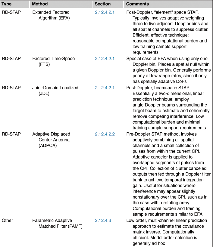
2.12.5 Application
In this section we consider the application of STAP to the important problem of radar detection in clutter. We employ the simulation models of Section 2.12.3 and some of the metrics from Section 2.12.2 to characterize the interference, algorithm performance, and STAP improvement over the non-adaptive processor.
Table 12.4 provides some of the parameters of the simulated, multi-channel radar system. Chosen parameters are similar to those of the Multi-Channel Airborne Radar Measurements (MCARM) system described in Section 2.12.8. Also, these are the same parameters used to generate Figures 12.1–12.3 in Section 2.12.1.

2.12.5.1 Interference characteristics
Using the models described in Section 2.12.3, we simulate clutter and noise for an eleven channel, thirty-two pulse airborne radar scenario. The clutter environment is homogeneous. Additional parameters are given in Table 12.4 and are similar in nature to a MCARM data collection referenced in Section 2.12.8. In this case, we simulated one CPI, where the aircraft experiences 6.78° of yaw. We focus our attention somewhat arbitrarily at a 32 km slant range for the analysis. Additionally, we simulated the eleven channel uniform linear array without array amplitude and phase errors. The antenna is steered to broad side: 0° azimuth and 0° elevation angle.
Figure 12.17 shows the PSD for this scenario. The PSD uses a Hanning weight in both space and time. The slight offset in peak clutter Doppler frequency in the look-direction from 0 Hz is due to platform yaw. The overall CNR is in the range of slightly greater than 50 dB. For comparison, Figure 12.18 shows the MVDR spectrum, clearly outlining the clutter angle-Doppler region of support. (Note: while MVDR provides units of power, it is widely known to be a poor estimator of the signal strength.) Figure 12.19 shows the eigenspectrum calculated using the known covariance matrix; the eigenspectrum displays the covariance matrix eigenvalues, sorted from largest to smallest. The noise eigenvalues are set to 0 dB, and those values greater than the noise floor correspond to the clutter signal. The largest eigenvalue is indicative of the CNR to within a few decibels, suggesting CNR in the range of 53–55 dB.
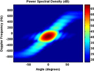
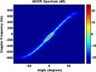
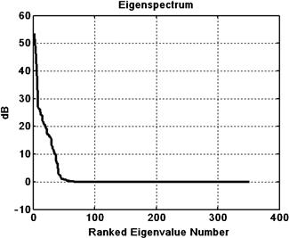
Considering the MVDR spectrum in Figure 12.18, we anticipate an optimal filter response that drives a deep null along the clutter angle-Doppler region of support. Figure 12.20 shows the optimal space-time filter response, steered to broadside and 400 Hz Doppler; the clutter null and peak gain is evident in the figure.

Figure 12.20 Optimal space-time frequency response, steered to array broadside and 400 Hz Doppler frequency.
Finally, Figure 12.21 shows the clairvoyant (known covariance) SINR loss, ![]() , over unambiguous Doppler
, over unambiguous Doppler ![]() in the broadside direction. The loss cut shows the impact of clutter on detection performance, with the null offset from 0 Hz due to the platform yaw. As seen from the figure, the null depth is slightly greater than 50 dB, consistent with the mainlobe CNR and the eigenspectrum of Figure 12.19. We will consider the performance of various STAP techniques relative to the clairvoyant SINR loss curve momentarily.
in the broadside direction. The loss cut shows the impact of clutter on detection performance, with the null offset from 0 Hz due to the platform yaw. As seen from the figure, the null depth is slightly greater than 50 dB, consistent with the mainlobe CNR and the eigenspectrum of Figure 12.19. We will consider the performance of various STAP techniques relative to the clairvoyant SINR loss curve momentarily.
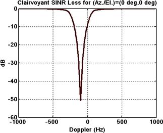
2.12.5.2 STAP algorithm performance
Based on the discussion in Section 2.12.4, we benchmark the performance of a number of STAP techniques using the scenario from the prior section. Again, we focus on a slant range of 32 km. Also, we consider clairvoyant loss, ![]() . For the homogeneous clutter scenario considered herein, the adaptive loss,
. For the homogeneous clutter scenario considered herein, the adaptive loss, ![]() , precisely follows the RMB rule: using sample support equal to twice the processor’s DoF yields, on average, 3 dB loss. The different techniques have different sample support requirements, based on their adaptive DoFs. An exception in this case involves the PAMF; the PAMF implementation averages over the pulse domain, and so can rely on less training data over range. However, this advantage is not unique to the PAMF, and other methods can also average over pulses (like the ADPCA technique) or employ smoothing techniques to effectively increase the sample support [43].
, precisely follows the RMB rule: using sample support equal to twice the processor’s DoF yields, on average, 3 dB loss. The different techniques have different sample support requirements, based on their adaptive DoFs. An exception in this case involves the PAMF; the PAMF implementation averages over the pulse domain, and so can rely on less training data over range. However, this advantage is not unique to the PAMF, and other methods can also average over pulses (like the ADPCA technique) or employ smoothing techniques to effectively increase the sample support [43].
Figure 12.22 compares the clairvoyant SINR loss of EFA, FTS, and JDL to the bound provided by the space-time optimal processor (STOP; the optimal space-time filter using the clairvoyant covariance matrix). In this case, the processors are configured as follows:
• FTS—uses all eleven channels and a Hanning weighting on the Doppler filters. Eleven adaptive spatial DoFs.
• EFA—uses all eleven spatial channels and three adjacent, Hanning-weighted Doppler filters. Thirty-three adaptive space-Doppler DoFs.
• JDL—uses three adjacent, uniform weighted spatial beams and three adjacent, Hanning-weighted Doppler filters. Nine total adaptive angle-Doppler DoFs. The beam spacing is three degrees (a little less than one-third of the full aperture 3 dB beamwidth).
From Figure 12.22, we find that EFA and JDL provide excellent performance potential relative to the achievable bound set by STOP. The FTS performance is disappointing, but not a surprise since this algorithm does not adaptively combine any temporal DoFs. One then might conclude JDL to be a better selection, since it only requires nine DoFs. However, the additional spatial DoFs afforded by EFA may prove beneficial when RFI or Doppler ambiguities are present. Thus, a number of analyses should take place before final algorithm selection.Figure 12.23 duplicates the aforementioned analysis for pre-Doppler STAP (ADPCA) and the PAMF. The processors are configured as follows:
• ADPCA—uses three adjacent pulses and all spatial channels for cancellation, then Doppler filters the resulting outputs using a Hanning weight. Thirty-three adaptive space-time DoFs. The implementation steers the temporal gain response to center the temporal steering vector null at −100 Hz, the center of mainlobe clutter.
• PAMF—uses a fourth-order filter model. No weighting is used on the Doppler steering vector.
The clairvoyant SINR loss curves in Figure 12.23 indicate that both ADPCA and PAMF provide very good performance, rivaling that of EFA and JDL in Figure 12.22.
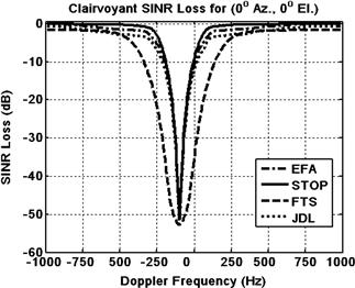

As a last example, Figure 12.24 shows the benchmark performance of the MWF using three, six, and twelve stages ![]() . As seen from the figure, the performance for
. As seen from the figure, the performance for ![]() or
or ![]() is poor, but very good capability is observed when
is poor, but very good capability is observed when ![]() . The computational loading of MWF, for the implementation used by the author, is significantly higher than the other methods examined.
. The computational loading of MWF, for the implementation used by the author, is significantly higher than the other methods examined.

2.12.5.3 STAP Comparison with nonadaptive solution
To conclude this section, we simply compare the performance of the space-time optimal filter to a nonadaptive processing scheme involving beamforming and Doppler processing. The nonadaptive filter implementation uses a Hanning temporal weight and uniform illumination spatially on receive. (Note: the transmit illumination uses a 30 dB Taylor weighting.) As seen from Figure 12.25, the space-time optimal filter provides a very significant performance advantage over the nonadaptive processor, thereby indicating the tremendous benefits of STAP.

2.12.5.4 Application summary
In this section we considered a typical airborne radar example. Clutter and noise models from Section 2.12.3 were used to simulate data snapshots and covariance matrices. The covariance matrices were used to assess the performance potential of several STAP techniques discussed in Section 2.12.4. From this analysis, we find that a number of the methods perform similarly well relative to the achievable performance bound. We caution the reader, however, that many other practical matters drive algorithm selection. Of the methods discussed, EFA often provides the best performance and greatest flexibility when considering a number of issues.
2.12.6 Challenges
Contemporary STAP research topics generally focus on challenges associated with covariance matrix estimation or mitigating computational burden. In this section we provide commentary on the former.
2.12.6.1 Heterogeneous clutter
Real world clutter environments are heterogeneous, thus tacitly undermining the IID assumption central to the development of (12.49) [44–46]. Heterogeneous clutter is a result of culturally-varying terrain type. Examples include: variation in clutter amplitude or spectral spread due to a mixture of clutter types; abrupt edges characteristic of clutter interfaces (e.g., between urban and rural regions); the presence of target-like signals in the training data (TSD) [45]; and, stationary, manmade objects resulting in strong, discrete responses. Each of the aforementioned effects is localized within the training set. Hence, the estimate of (12.49) captures the average behavior of the training data, thus potentially appearing mismatched to any particular cell under test. This mismatch translates to an erroneous, adaptive response relative to the optimal condition. SINR loss or threshold bias results in such instances. References [44–46] characterize in detail the nature of such system degradation.
As an example, distributed clutter is typically site-specific: the clutter reflectivity varies as a function of range and angle due to changes in the terrain features. Equation (12.70) accommodates site-specific simulation by modifying the term, ![]() , through access of a database to determine the clutter RCS,
, through access of a database to determine the clutter RCS, ![]() , in (12.67)–(12.69) (where the reference to the qth range ambiguity is added). Figure 12.26 compares actual and site-specific simulation of UHF radar data taken in the Delaware-Maryland-Virginia (Delmarva) Peninsula region; this region is dominated by rural clutter, bodies of water and rivers, and also covered by a number of roadways. As seen from Figure 12.26, the range and cross-range (Doppler, or angle) variation of the clutter response is evident and predictable. The clutter variation shown is one source of heterogeneity leading to covariance matrix estimation error.
, in (12.67)–(12.69) (where the reference to the qth range ambiguity is added). Figure 12.26 compares actual and site-specific simulation of UHF radar data taken in the Delaware-Maryland-Virginia (Delmarva) Peninsula region; this region is dominated by rural clutter, bodies of water and rivers, and also covered by a number of roadways. As seen from Figure 12.26, the range and cross-range (Doppler, or angle) variation of the clutter response is evident and predictable. The clutter variation shown is one source of heterogeneity leading to covariance matrix estimation error.
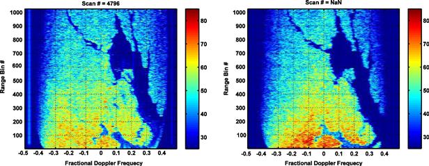
Figure 12.26 Comparison of measured (left) and simulated (right) multichannel UHF radar data (colorbar in decibels) (after [47]). © 2006 IEEE
Table 12.5 provides a summary of various sources of heterogeneous clutter and their impact on STAP performance. Of the effects listed, it is observed that target-like signals corrupting the secondary (training) data (TSD) and clutter discretes tend to lead to the greatest performance loss.
Table 12.5
Summary of Heterogeneous Clutter and STAP Impact
| Source | Description | Impact on STAP |
| Spatially-varying, distributed clutter RCS | Range-angle variation in clutter RCS leads to varying power across clutter angle-Doppler region of support | Over- or undernulled clutter. Overnulled clutter can lead to signal cancellation, whereas undernulling leads to clutter residue and degraded SINR |
| Spatially-varying, distributed clutter spectral spread | Range-angle variation of intrinsic clutter motion varies spectral spread across clutter angle-Doppler region of support | Training on regions where ICM is less than that of the application region leads to insufficient null width and an increase in clutter residual, whereas regions with ICM less than that present in the training set experience suppression of low speed targets |
| Clutter edges and shadowing | Gross variation in clutter type (e.g., land-sea interface) or regions of extended obscuration, predominantly in the mainlobe direction | Over- or undernulled clutter |
| Clutter discretes | Stationary objects with relatively large RCS, often manmade objects such as cars, utility poles, etc., also includes extended discretes, such as fence lines and train tracks | Increased false alarm rate, upward threshold bias leading to increase in missed detections |
| Target-like signals | Vehicles on roadways and within airspace, predominantly through the mainbeam | Signal cancellation due to nulling off the clutter ridge in angle-Doppler locations consistent with targets of interest |
A variety of techniques have been developed to enhance STAP detection performance given the challenges of heterogeneous clutter. We summarize some of the available methods in Table 12.6. As discussed in [47], the different approaches fall in one of two categories: indirect or direct. The indirect methods attempt to manipulate the training set to improve the covariance matrix estimate, oftentimes using knowledge of the platform motion or surrounding terrain or operating environment, whereas the direct methods attempt to modify the filter response using models and ancillary information. Both indirect and direct methods attempt to improve the instantaneous adaptive filter response to minimize heterogeneous clutter residue at the filter output; in this manner, STAP performance in complex, heterogeneous environments can approach that attainable in a homogeneous setting.
Table 12.6
STAP Techniques to Mitigate the Impact of Heterogeneous Clutter on Detection Performance
| Technique | Description | Reference |
| Nonhomogeneity Detector (NHD) | Data-dependent screening measure, tests training data for similarity to the average, selects homogeneous training samples | [50–52] |
| Power Selected Training (PST) | Data-dependent screening measure, selects training samples strongest in power to drive null as deeply as possible | [53,54] |
| Power Comparable Training (PCT) | Data-dependent screening measure, sorts data into tiles of similar power levels to match training data to cell under test | [55] |
| Power Variable Training (PVT) | Scale the power of the estimated covariance matrix’s dominant (clutter) subspace to match the power level in the cell under test, requires eigendecomposition | [56] |
| Map-aided training | Uses mapping data and distance measures to screen training samples | [24,57] |
| Covariance matrix taper (CMT) | Purposely spreads the estimated clutter response to increase null width | [58] |
| Subaperture smoothing | Exploits similar covariance structure among sub-apertures of a uniformly sampled spatial or temporal aperture to enhance the quantity of homogeneous training samples | [43,59] |
| Nonlinear, nonadaptive STAP | Employs a model of the clutter covariance matrix to suppress clutter | [60] |
| Color loading | Adds a scaled clutter covariance model to the covariance matrix estimate to emphasize the anticipated clutter response and enable localized training | [61,62] |
| Discrete Matched Filter (DMF) | Coherently removes clutter discrete signals using a modified version of the CLEAN algorithm | [47] |
| Signal and Clutter as Highly Independent Structured Modes (SCHISM) | Coherently removes distributed clutter returns using a modified version of the CLEAN algorithm | [63] |
| Adaptive Coherence Estimator (ACE) | Incorporates a statistical measure of the “whiteness” of the clutter residue in a particular cell under test to suppress clutter discretes? | [64] |
| Knowledge-Aided Parametric Covariance Estimation (KAPE) | Estimates parameters of a validated covariance matrix model, including clutter amplitude, spread, mainlobe centroid, and error components of the array manifold | [16,65] |
As an example of the degradation of heterogeneous interference effects, and the improvement potential of available STAP techniques, Figure 12.27 compares detection rates using MCARM Flight 5, Acquisition 575 data using block training (bins 200–320) versus intelligent training and filter selection (ITFS, [47]), where maps facilitate training data excision in regions overlaying certain roadways. As seen from the figure, TSD leads to excessive, additional loss in the lobed regions near ![]() 20 m/s; removing a specific highway using ITFS—as noted in the figure’s legend—fully mitigates this loss, raising the detection rate from roughly 55% to 98%.
20 m/s; removing a specific highway using ITFS—as noted in the figure’s legend—fully mitigates this loss, raising the detection rate from roughly 55% to 98%.

Figure 12.27 Estimated detection probability improvement over Doppler frequency using KA training on MCARM data (after [24]). © 2004 IEEE
2.12.6.2 Nonstationary clutter
STAP maximizes SINR by filtering ground clutter in the angle-Doppler domain. Radar geometry determines the filter null location in this higher-dimensional space. When the null location varies over range, the adaptive filter produces an incorrect frequency response. In the monostatic radar case, the angle-Doppler region of support can exhibit range variation when the velocity vector and array normal are non-orthogonal. This occurs for forward-looking arrays, or under conditions when the platform is yawed [48,49].
In sidelooking array radar, the spatial frequency measured by a uniform linear array is proportional to the corresponding Doppler frequency of a stationary clutter patch on the Earth’s surface. Specifically, normalized Doppler, ![]() , can be written
, can be written
![]() (12.138)
(12.138)
where ![]() is the platform velocity in the direction orthogonal to the array normal, T is PRI,
is the platform velocity in the direction orthogonal to the array normal, T is PRI, ![]() is wavelength,
is wavelength, ![]() is the cone angle measurement from the platform centerline to the clutter patch location, d is channel spacing, and
is the cone angle measurement from the platform centerline to the clutter patch location, d is channel spacing, and ![]() is spatial frequency. Spatial frequency is given by
is spatial frequency. Spatial frequency is given by
![]() (12.139)
(12.139)
Physically, the clutter iso-Doppler contours and the array beam traces align, translating to angle-Doppler behavior that is range invariant.
In the non-sidelooking radar case, the beam traces and iso-Dopplers of the ground clutter returns misalign at some ranges, mainly those where the range divided by the altitude is less than five [18,19]. The variation of the clutter response through the training set leads to an adaptive filter response with incorrect null placement, leading to increased clutter residue and degraded detection performance. References [48,49] discuss effective compensation methods.
Range varying angle-Doppler loci further exacerbates culturally induced heterogeneous clutter effects. For example, residue from clutter discretes further increase in the presence of adaptive filter null migration associated with the non-stationary clutter mechanism described in this section.
2.12.6.3 Bistatic STAP
Bistatic STAP development received considerable attention in the early-to-mid 2000s. Airborne bistatic radar involves a moving transmitter and receiver separated a considerable distance. The bistatic geometry and independent motion between transmitter and receiver leads to significant angle-Doppler variation over range [75,72].
Table 12.7 summarizes a number of recently developed bistatic STAP techniques, including a description of the approach and germane references. As seen from the table, the methods generally fall in one of three categories: localized processing (or training); data pre-warping, prior to STAP application; and, time-varying weights. Several of the bistatic STAP methods in Table 12.7 have proven extraordinarily effective, restoring performance to levels similar to that achievable in homogeneous clutter environments.
Table 12.7
Summary of Bistatic STAP Methods
| Bistatic STAP approach | Description | Reference |
| Localized processing | Simple strategy, attempts to choose training data in the vicinity of the cell under test to minimize nonstationary impacts | [66,67] |
| Time-varying weights | Employs truncated Taylor series expansion of the weight vector, presumes linear evolution in the weight vector elements over range | [68,69] |
| Doppler warping | Aligns a point of the clutter ridge for each bistatic range to a designated reference point (e.g., 0 Hz Doppler) using a range-varying, complex modulation prior to STAP application | [49] |
| Higher-order Doppler warping | Aligns sections of the clutter ridge to a reference ridge using a range varying modulation, a multi-point extension of the Doppler warping method prior to STAP application | [70] |
| Angle-Doppler compensation | Aligns “spectral centers,” or regions of maximum angle-Doppler return, over range using a complex, range-varying, space-time modulation prior to STAP application | [71] |
| Adaptive angle-Doppler compensation | Derives key information on clutter range variation directly from the data, applies a complex, space-time, range-varying modulation to the data to algin dominant clutter subspaces prior to STAP application | [72,73] |
| Registration of “direction-Doppler curves” | Uses curve fitting methods to warp the power spectral density of a given range sum to a reference prior to STAP application | [74] |
2.12.6.4 Conformal array STAP
A conformal array’s shape is compliant with the contours of the radar bearing platform. For example, Figure 12.28 depicts conformal antenna elements mounted to a chined nose cone; the short lines emanating from each dot representing an antenna element indicate the surface normal.
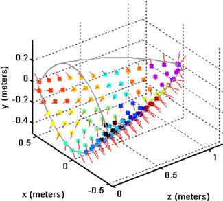
The curvature of the conformal array, coupled with the look-direction relative to the velocity vector, results in a nonstationary clutter angle-Doppler response [76–78]. SINR loss resulting from the nonstationary clutter response rivals that seen in bistatic radar examples. Hersey et al. [76] discusses several solutions to mitigate nonstationary clutter behavior based on adaptations of solutions developed for bistatic STAP implementation, including localized processing, localized processing with time-varying weights, angle-Doppler warping, and higher-order angle-Doppler warping. Additionally, Hersey et al. [76] develops a method called equivalent uniform linear array transformation which attempts to resample the data to a linear configuration. The conformal array STAP methods in [76] lead to significant performance enhancement.
2.12.7 Implementation
We discuss a generic, STAP-based, airborne radar detection architecture in this section. A flow diagram of the detection process is given in Figure 12.29.
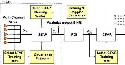
STAP is applied at the CPI level. As a result of target fading, the MTI radar typically transmits bursts of pulses at several different frequencies, where each burst comprises the CPI. Being a coherent signal processing technique, STAP operates on each CPI as indicated in the figure, essentially generating a range-Doppler map (RDM) at a receive angle consistent with the transmit direction: a space-time snapshot for each range bin, ![]() , is processed using a space-time weighting steered to a given angle and Doppler to yield a single pixel in the RDM,
, is processed using a space-time weighting steered to a given angle and Doppler to yield a single pixel in the RDM, ![]() . Each CPI is processed, generating aligned RDMs; the alignment may require additional processing steps, such as motion compensation. Then, the RDMs at the different frequencies are noncoherently summed in a step called post-detection integration (PDI; also called noncoherent addition, NCA). PDI boosts detection performance by taking advantage of the purposeful decorrelation created by frequency hopping to avoid target fading that adversely affects operation using a single coherent dwell. Frequency hopping forces the target to take on a Swerling 2 characteristic [1,7].
. Each CPI is processed, generating aligned RDMs; the alignment may require additional processing steps, such as motion compensation. Then, the RDMs at the different frequencies are noncoherently summed in a step called post-detection integration (PDI; also called noncoherent addition, NCA). PDI boosts detection performance by taking advantage of the purposeful decorrelation created by frequency hopping to avoid target fading that adversely affects operation using a single coherent dwell. Frequency hopping forces the target to take on a Swerling 2 characteristic [1,7].
After PDI, a detection threshold is set using a constant false alarm rate (CFAR) algorithm; the CFAR algorithm multiplies an estimate of the residual interference power by a threshold multiplier in an attempt at achieving a constant false alarm rate [1]. Pixel values crossing the detection threshold are declared targets. The signal processor then estimates the bearing and Doppler frequency of the threshold crossing generally using a maximum likelihood estimator. The corresponding SINR, bearing, Doppler, and range—among other potential characteristics—for each detection is then passed to an analyst or an automatic tracker. Figure 12.29 is meant to show the basic processing steps; it is common to incorporate additional functionality to cope with clutter heterogeneity or target motion through resolution cells, for instance.
The selection of the scalar, ![]() , in (12.44) is an important, practical consideration. It is common to use the adaptive matched filter (AMF) normalization [79],
, in (12.44) is an important, practical consideration. It is common to use the adaptive matched filter (AMF) normalization [79],
 (12.140)
The AMF normalization sets the residual interference-plus-noise floor to unity as ![]() , viz.
, viz.
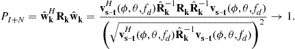 (12.141)
The AMF normalization accommodates variable training intervals and other segmentation of the weight estimation and application over range, minimizing shifts in the mean, residual interference-plus-noise power that otherwise leads to threshold bias and increased false alarm rate. More specifically, assuming the segmented interference-plus-noise environment is IID, the AMF normalization possesses CFAR properties: as power fluctuates from one weight application region to the next, the filter output is scaled by the inverse of the residual interference-plus-noise power so that a fixed detection threshold maintains a constant false alarm rate. This is seen by examining the AMF decision statistic,
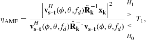 (12.142)
where ![]() is a fixed decision threshold. Moving the denominator of the decision statistic to the right, (12.142) is interpreted as the square of the filter output (the numerator term) compared to a threshold multiplier,
is a fixed decision threshold. Moving the denominator of the decision statistic to the right, (12.142) is interpreted as the square of the filter output (the numerator term) compared to a threshold multiplier, ![]() , scaled by the residual interference-plus-noise output power. This is the conventional view of CFAR in radar signal processing.
, scaled by the residual interference-plus-noise output power. This is the conventional view of CFAR in radar signal processing.
A virtually identical formulation of the AMF result is given in [80] and referred to as Modified Sample Matrix Inversion (MSMI).
A maximum likelihood estimate for target bearing and Doppler integrates seamlessly with the architecture in Figure 12.29 and use of the AMF normalization. This can be seen by expressing the alternative hypothesis of (12.2) as
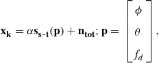 (12.143)
where ![]() is a complex constant, and
is a complex constant, and ![]() is the interference-plus-noise (total noise) vector. The objective is to estimate
is the interference-plus-noise (total noise) vector. The objective is to estimate ![]() with
with ![]() . Since
. Since ![]() , the joint probability density function (pdf) is
, the joint probability density function (pdf) is
![]() (12.144)
(12.144)
Given the likelihood function defined by (12.144), we first require an estimate for the complex constant. Equation (12.144) is maximal when
![]() (12.145)
(12.145)
is minimal. Differentiating (12.145) and setting the result to zero yields
 (12.146)
Substituting (12.146) into (12.145) leads to
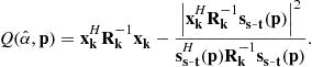 (12.147)
Differentiating (12.147) with respect to ![]() and setting the result to zero yields the maximum likelihood estimate (MLE),
and setting the result to zero yields the maximum likelihood estimate (MLE), ![]() . Consequently, the estimator is [81]
. Consequently, the estimator is [81]
 (12.148)
The MLE takes the form of an AMF normalized STAP cost surface and in practice ![]() replaces
replaces ![]() . Implementing the estimator requires a very fine grid search to find the peak of the likelihood function (via the MLE approach). The grid search—which essentially amounts to stepping the space-time steering vector over potential target angles and Dopplers—is computationally burdensome and can be sub-optimum. Specifically, if the step size is too large, the estimator can exhibit bias and increased variance. For this reason, numerical approximations to the MLE, which exhibit good practical performance, are commonly used.
. Implementing the estimator requires a very fine grid search to find the peak of the likelihood function (via the MLE approach). The grid search—which essentially amounts to stepping the space-time steering vector over potential target angles and Dopplers—is computationally burdensome and can be sub-optimum. Specifically, if the step size is too large, the estimator can exhibit bias and increased variance. For this reason, numerical approximations to the MLE, which exhibit good practical performance, are commonly used.
When processing multiple CPIs, the MLE appears as the sum of the individual cost surfaces at each frequency, where each cost surface takes the form of the term in parentheses in (12.148). An equivalent development for the multistatic radar case is given in [82].
STAP remains computationally challenging to implement. The weight calculation generally takes place in either the voltage domain using QR decomposition (QRD) or in the power domain using Cholesky factorization. Calculating the weight vector using QRD in the voltage domain seems favorable, since it essentially doubles the dynamic range in decibels over the power domain solution and avoids explicitly forming outer products in the covariance estimation step. Cholesky factorization in the power domain is also a common approach when considering all the details of real-time implementation on specific computing devices.
2.12.8 STAP data collection programs
In this section we highlight some measured data collection programs.
2.12.8.1 Multichannel Airborne Radar Measurements (MCARM)
In the mid-1990s, the US Air Force Rome Laboratory (now the Air Force Research Laboratory) contracted with Westinghouse Corporation (now Northrop Grumman) to build and fly a multi-channel, L-band radar under the Multi-Channel Airborne Radar Measurements (MCARM) Program [83]. The MCARM program produced a meaningful collection of multi-channel radar data over a range of clutter conditions to evaluate the performance potential of STAP and support continued technology development.
The salient parameters of the MCARM system are given in Table 12.8. As seen from the table, the system has relatively high peak power, an electrically modest aperture at L-band, relatively low range resolution, and built-in features to calibrate the antenna and radio frequency front-end. Additionally, as Figure 12.30 shows, MCARM has a highly flexible array configuration, supporting a range of study options, including planar array configuration, uniform linear array, and sum and difference channel analyses. Figure 12.31 shows the region of the Eastern United States—the Delmarva Peninsula—where several acquisitions were collected during MCARM Flight 5. As previously mentioned, this region is relatively flat, dominated by rural clutter and water, and covered by a number of roadways, including several highways. Results from Acquisition 575, in particular, have been presented in a number of papers, starting with [50].
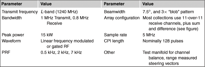
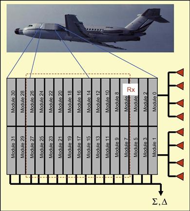
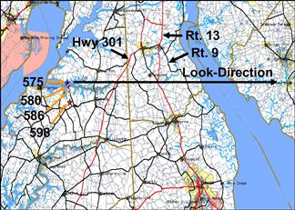
It is known that some of the MCARM acquisitions were previously made publicly releasable, as described in [84]. The Air Force Research Laboratory, Sensors Directorate, maintains the MCARM database.
2.12.8.2 Naval Research Laboratory (NRL) database
The Naval Research Laboratory (NRL) Adaptive Array Flight Test Database is decribed in [85]. Table 12.9 provides some flight test parameters. According to [85], the effort remarkably consisted of over thirty flights, collecting in excess of 2500 data files. Data were collected predominantly in the mountainous regions of Virginia and West Virginia, with urban clutter data collected in the vicinity of Washington, DC, and rural clutter data collected in North Carolina, Georgia, Ohio, and Indiana. Sea clutter data were collected over the Atlantic Ocean, east of Virginia, with some littoral clutter data also recorded.
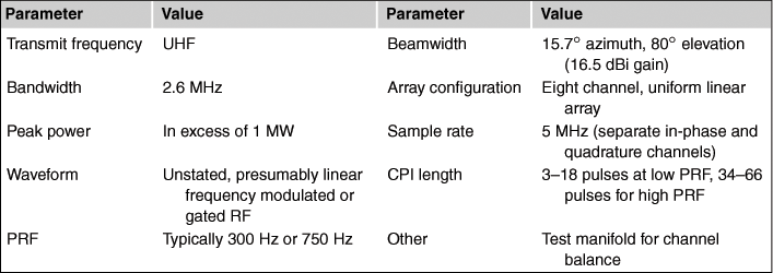
Lee and Staudaher [85] indicates a database was constructed, with data formatted for MATLAB® analysis, with the intent “that the database will provide the adaptive signal processing community with a valuable tool for validating both existing and future adaptive algorithms.”
2.12.8.3 Mountaintop database
According to [86,87], the Mountaintop Program goal sought to advance airborne early warning radar technology. Collection of surveillance radar clutter and jamming data from mountaintops at White Sands Missile Range, New Mexico, and Pacific Missile Range Facility, Hawaii, served as central objectives in this effort. The Mountaintop radar, known as the Radar Surveillance Technology Experimental Radar (RSTER), employed an inverse displaced phase center antenna (IDPCA) technique to give the appearance of platform motion. RSTER parameters are given in Table 12.10. In IDPCA, the system steps the transmit location to one (or three) of eighteen total transmit antenna columns.
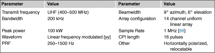
According to [87], Mountaintop RSTER data are archived using the Common Research Environment for STAP (CREST) database. Additionally, some data is accessible at the IEEE Signal Processing Information Base at Rice University [88].
2.12.8.4 Knowledge-aided sensor signal processing and expert reasoning (KASSPER) data
Improving the performance of STAP in complex clutter environments served as a primary aim of the DARPA KASSPER Program [89]. Under this program, DARPA funded the creation of several sets of synthetic, multichannel, multi-pulse, multi-range datacubes at X-band and L-band. The L-band datacube—KASSPER datacube #1, or KDC #1—is publicly releasable and was provided to attendees at the 2002 DARPA KASSPER Workshop [90]. Many of the L-band data parameters resemble those of the MCARM system described in Table 12.8, the exception mainly being the use of an eleven channel uniform linear array and typically fewer pulses in the CPI. Each of the KASSPER datacubes is a result of high-fidelity, site-specific clutter simulation. Dense moving targets are present in the data. A unique aspect of the simulation is the availability of truth information, including known covariance matrices on a range cell basis and target location data for some of the datasets (including the L-band datacube and some of the X-band cases).
Figure 12.32 shows MVDR spectra for KDC #1 range bins 102 and 500, with pre-steering applied to the antenna boresight. Additionally, the KASSPER datacubes included simulated antenna errors, with the true error vector provided with the data sets; the two-dimensional MVDR spectra in Figure 12.32 employ knowledge of the precise array manifold.

2.12.9 Summary
This tutorial describes a number of key aspects of STAP. Naturally, it is challenging to fully cover all the details of a topic so vast. Our goals for this effort are simpler: provide a concise, single reference to augment the available text books, reports, and papers on this important subject and highlight some of the more significant developments within the research community.
In this tutorial, we describe a number of approaches to design optimal filters. Of the methods described, all end up being closely related and ultimately maximize the probability of detection for a fixed probability of false alarm. We then discuss signal models for clutter, noise, radio frequency interference and target. These models form the basis for STAP algorithm development and analysis. STAP, as it turns out, refers to a collection of a number of practical techniques; we discuss several major algorithm themes, include post-Doppler STAP, pre-Doppler STAP, and parametric STAP. We further discuss a number of eigen- or subspace-based cancellation architectures, including Principle Components Inverse, the cross spectral metric, and the Multi-Stage Wiener Filter.
Using the simulation models and algorithm descriptions, we then characterize the performance of the various methods using SINR loss, a key performance metric in the STAP community, using a homogeneous clutter scenario. We find that, for the approach taken, all but one of the methods provides similarly good performance relative to the bound set by the optimal space-time filter.
Key challenges in the STAP research community center on modifying textbook principles to support real-world application. Invariably, the accurate estimation of the unknown clutter covariance matrix and implementing the adaptive filter in a real-time computing environment are driving considerations. In this vein, we briefly discuss the challenges of STAP application in heterogeneous clutter environments, for bistatic or conformal array configurations, and in the presence of otherwise nonstationary clutter.
A number of concepts are concisely summarized in Section 2.12.7, where we describe the end-to-end implementation of a basic MTI radar processor. STAP normalization and target parameter estimation is considered in this section.
We conclude the discussion by summarizing several STAP data collection programs, the characteristics of the various radar systems, and the type of data collected or generated.
Symbols and notation
We provide a key to some common notation used in this paper.
L number of available range bins
T pulse repetition interval (s)
![]() platform velocity vector (m/s, m/s, m/s)
platform velocity vector (m/s, m/s, m/s)
![]() hypothesized spatial steering vector
hypothesized spatial steering vector
![]() hypothesized temporal steering vector
hypothesized temporal steering vector
![]() hypothesized space-time steering vector
hypothesized space-time steering vector
![]() spatial data snapshot, kth range cell, nth pulse
spatial data snapshot, kth range cell, nth pulse
![]() space-time data snapshot, kth range cell
space-time data snapshot, kth range cell
![]() clutter space-time snapshot, kth range cell
clutter space-time snapshot, kth range cell
![]() RFI space-time snapshot, kth range cell
RFI space-time snapshot, kth range cell
![]() uncorrelated noise space-time snapshot, kth range cell
uncorrelated noise space-time snapshot, kth range cell
![]() target space-time snapshot, kth range cell
target space-time snapshot, kth range cell
![]() null-hypothesis covariance matrix (kth range cell)
null-hypothesis covariance matrix (kth range cell)
![]() receive noise covariance matrix
receive noise covariance matrix
![]() null-hypothesis covariance estimate, kth range cell
null-hypothesis covariance estimate, kth range cell
Acronyms
Following is a list of common acronyms:
ADPCA adaptive displaced phase center antenna
CFAR constant false alarm rate
CPI coherent processing interval
CREST Common Research Environment for STAP
FLAR forward-looking array radar
GLSC generalized sidelobe canceler
GMTI ground moving target indication
IDPCA inverse displaced phase center antenna processing
IID independent and identically distributed
KASSPER Knowledge-Aided Sensor Signal Processing and Expert Reasoning
MCARM Multi-Channel Airborne Radar Measurements
MCLP multichannel linear prediction
MDV minimum detectable velocity
MLE maximum likelihood estimate
MMSE minimum mean square error
MSMI modified sample matrix inversion
MPE minimum power eigencanceler
MNE minimum norm eigencanceler
MVDR minimum variance distortionless response
pdf probability density function
PDI post-detection integration
RFI radio frequency interference
RD-STAP reduced-dimension STAP
RSTER Radar Surveillance Technology Experimental Radar
SINR signal-to-interference-plus-noise ratio
STAP space-time adaptive processing
STOP space-time optimal processing
TSD targets in the secondary data
Relevant Theory: Statistical Signal Processing and Array Signal Processing
See Vol. 3, Chapter 5 Distributed Signal Detection
See Vol. 3, Chapter 19 Array Processing in the Face of Nonidealities
References
1. Richards M, ed. Principles of Modern Radar: Basic Principles. North Carolina: Sci-Tech Publishing, Inc.; 2010.
2. DiFranco JV, Rubin WL. Radar Detection. Dedham, MA: Artech-House; 1980.
3. Brennan LE, Reed IS. Theory of adaptive radar. IEEE Trans AES. 1973;9(2):237–252.
4. I.S. Reed, A brief history of adaptive arrays, Sudbury/Wayland Lecture Series (Raytheon Div. Education), Notes, 23 October 1985.
5. Klemm R. Doppler properties of airborne clutter. In: Proceedings of the Research and Technology Organization, North Atlantic Treaty Organization (RTO-NATO) Lecture Series 228—Military Applications of Space-Time Adaptive Processing, RTO-ENP-027. September 2002;2-1–2-24.
6. Entzminger JN, Fowler CA, Kenneally WJ. JointSTARS and GMTI: past, present and future. IEEE Trans AES. 1999;35(2):748–761.
7. Skolnik MI. Introduction to Radar Systems. second ed. New York, NY: McGraw Hill; 1980.
8. Levanon N. Radar Principles. New York: John Wiley & Sons; 1988.
9. Melvin WL. A STAP overview. Willett Peter, ed. IEEE AES Systems Magazine—Special Tutorials Issue. 2004;19(1):19–35.
10. J. Ward, Space-Time Adaptive Processing for Airborne Radar, Lincoln Laboratory Technical, Report, ESC-TR-94-109, December 1994.
11. Guerci JR. Space-Time Adaptive Processing for Radar. Norwood, MA: Artech House; 2003.
12. Haykin S. Adaptive Filter Theory. third ed. Upper Saddle River, NJ: Prentice-Hall; 1996.
13. Johnson DH, Dudgeon DE. Array Signal Processing: Concepts and Techniques. Englewood Cliffs, NJ: Prentice-Hall; 1993.
14. Griffiths LJ, Jim CW. An alternative approach to linearly constrained adaptive beamforming. IEEE Trans Antenn Propag. 1982;30(1):27–34.
15. Novak LM, Sechtin MB, Cardullo MJ. Studies of target detection algorithms that use polarimetric radar data. IEEE Trans AES. 1989;25(2):150–165.
16. Melvin WL, Showman GA. Knowledge-aided parametric covariance estimation. IEEE Trans AES 2006;1021–1042.
17. Reed IS, Mallett JD, Brennan LE. Rapid convergence rate in adaptive arrays. IEEE Trans AES. 1974;10(6):853–863.
18. Klemm R. Space-time adaptive processing: principles and applications. In: IEE Radar, Sonar, Navigation and Avionics 9. IEE Press 1998.
19. Klemm R. Principles of space-time adaptive processing IEE Radar, Sonar, Navigation and Avionics 12 second ed. UK: IEE Press; 2002; (Note: a 3rd edition of this text, published in 2006, is also available.).
20. Barton D. Land clutter models for radar design and analysis. Proc IEEE. 1985;73(2):198–204.
21. Billingsley JB. Low-Angle Radar Land Clutter: Measurements and Empirical Models. William Andrew Publishing, Inc. 2002.
22. Mailloux RJ. Phased Array Antenna Handbook. Boston, MA: Artech House; 1994.
23. Zatman M. How narrow is narrowband? IEE Proc Radar Sonar Navig. 1998;145(2):85–91.
24. Melvin WL, Showman GA, Guerci JR. A knowledge-aided GMTI detection architecture. Proceedings of the 2004 IEEE Radar Conference, Philadelphia, PA. 2004;26–29 ISBN: 0-7803-8235-8.
25. Rabinkin DV, Pulsone NB. Subband-domain signal processing for radar array systems. In: Proceedings of the SPIE Conference on Advanced Signal Processing Algorithms, Architectures, and Implementations IX, Denver, CO. July 1999;174–187.
26. Klemm R. Adaptive clutter suppression for airborne phased array radar. Proc IEE. 1983;130(1):125–132.
27. Gierull CH, Balaji B. Minimal sample support space-time adaptive processing with fast subspace techniques. IEE Proc Radar Sonar Navig. 2002;149(5):209–220.
28. Gabriel WF. Using spectral estimation techniques in adaptive processing antenna systems. IEEE Trans Antenn Propag. 1986;34(3):291–300.
29. Tufts DW, Kirsteins I, Kumaresan R. Data-adaptive detection of a weak signal. IEEE Trans AES. 1983;19(2):313–316.
30. Haimovich AM. The Eigencanceler: adaptive radar by eigenanalysis methods. IEEE Trans AES. 1996;32(2):532–542.
31. Hung EKL, Turner RM. A fast beamforming algorithm for large arrays. IEEE Trans AES. 1983;19(4):598–607.
32. Carlson BD. Covariance matrix estimation errors and diagonal loading in adaptive arrays. IEEE Trans AES. 1988;24(4):397–401.
33. Guerci JR, Goldstein JS, Reed IS. Optimal and adaptive reduced-rank STAP. IEEE Trans AES. 2000;36(2):647–661.
34. Berger SD, Welsh BM. Selecting a reduced-rank transformation for STAP—a direct form perspective. IEEE Trans AES. 1999;35(2):722–729.
35. Goldstein JS, Reed IS, Zulch PA. Multistage partially adaptive STAP CFAR detection algorithm. IEEE Trans AES. 1999;35(2):645–661.
36. DiPietro RC. Extended factored space-time processing for airborne radar. In: Proceedings of the 26th Asilomar Conference, Pacific Grove, CA. October 1992;425–430.
37. Wang H, Cai L. On adaptive spatial-temporal processing for airborne surveillance radar systems. IEEE Trans AES. 1994;30(3):660–670.
38. Brown R, Wicks M, Zhang Y, Zhang Q, Wang H. A space-time adaptive processing approach for improved performance and affordability. In: 1996;321–326. Proceedings of the 1996 IEEE National Radar Conference, Ann Arbor, Michigan, May 13–16 .
39. Klemm R. Antenna design for airborne MTI. In: Proceedings of the Radar 92, Brighton, UK. October 1992;296–299.
40. Blum R, Melvin W, Wicks M. An analysis of adaptive DPCA. In: 1996;303–308. Proceedings of the 1996 IEEE National Radar Conference, Ann Arbor, Michigan, May 13–16 .
41. Roman JR, Rangaswamy M, Davis DW, Zhang Q, Himed B, Michels JH. Parametric adaptive matched filter for airborne radar applications. IEEE Trans AES. 2000;36(2):677–692.
42. G.A. Showman, Personal, communication, 13 July 2003.
43. Fante RL, Barile EC, Guella TP. Clutter covariance smoothing by subaperture averaging. IEEE Trans AES. 1994;30(3):941–945.
44. Melvin WL. Space-time adaptive radar performance in heterogeneous clutter. IEEE Trans AES. 2000;36(2):621–633.
45. Melvin WL, Guerci JR. Adaptive detection in dense target environments. Proceedings of the 2001 IEEE Radar Conference Atlanta, GA, May 1–3 2001;187–192.
46. Melvin WL. STAP in heterogeneous clutter environments. In: IEE Press 2004;Klemm R, ed. The Applications of Space-Time Processing, IEE Radar, Sonar, Navigation and Avionics. 9.
47. Melvin WL, Guerci JR. Knowledge-aided sensor signal processing: a new paradigm for radar and other sensors. IEEE Trans AES 2006;983–996.
48. Kreyenkamp O, Klemm R. Doppler compensation in forward-looking STAP radar. IEE Proc Radar Sonar Navig. 2001;148(5):252–258.
49. Borsari G. Mitigating effects on STAP processing caused by an inclined array. In: Proceedings of the 1998 IEEE Radar Conference, Dallas, Tx. May 1998;135–140.
50. Melvin WL, Wicks MC, Brown RD. Assessment of multichannel airborne radar measurements for analysis and design of space-time processing architectures and algorithms. In: Proceedings of the 1996 IEEE National Radar Conference, Ann Arbor, Michigan, May 13–16,. 1996;130–135.
51. Melvin WL, Wicks MC. Improving practical space-time adaptive radar. In: Proceedings of the 1997 IEEE National Radar Conference, Syracuse, New York, May 13–15. 1997;48–53.
52. Chen P, Melvin WL, Wicks MC. Screening among multivariate normal data. J Multivariate Anal. 1999;69:10–29.
53. Rabideau DJ, Steinhardt AO. Improving the performance of adaptive arrays in non-stationary environments through data-adaptive training. Proceedings of the 30th Asilomar Conference, Pacific Grove, CA. November 1996;3–6:75–79.
54. Rabideau DJ, Steinhardt AO. Improved adaptive clutter cancellation through data-adaptive training. IEEE Trans Aerosp Electron Syst. 1999;35(3):879–891.
55. G.A. Showman, W.L. Melvin, Knowledge-aided discrete removal techniques, in: Proceedings of the 2005 DARPA ISIS/KASSPER Workshop, Las Vegas, NV, 22–24 February 2005, CD ROM.
56. Pulsone N. Improving ground moving target indication performance. In: Proceedings of the DARPA/AFRL KASSPER Workshop, 14–16 April 2003, Las Vegas, NV. 2003.
57. Berger SD, Melvin WL, Showman GA. Map-aided secondary data selection. In: Proceedings of the 2007 IEEE Radar Conference, Boston, MA. April 2007.
58. Guerci JR. Theory and application of covariance matrix tapers for robust adaptive beamforming. IEEE Trans Signal Process. 1999;47(4):977–985.
59. Pillai SU, Kim YL, Guerci JR. Generalized forward/backward subaperture smoothing techniques for sample starved STAP. IEEE Trans Signal Process. 2000;48(12):3569–3574.
60. Farina A, Lombardo P, Pirri M. Nonlinear nonadaptive space-time processing for airborne early warning radar. IEE Proc Radar Sonar Navig. 1998;145(1):9–18.
61. Bergin JS, Teixeira CM, Techau PM, Guerci JR. STAP with knowledge-aided data pre-whitening. In: Proceedings of the 2004 IEEE Radar Conference. April 2004;289–294.
62. Bergin JS, Teixeria CM, Techau PM, Guerci JR. Space-time beamforming with knowledge-aided constraints. In: Proceedings of the 2003 Adaptive Sensor Array Processing Workshop, MIT Lincoln Laboratory, Lexington, MA, March. 2003.
63. Letgers GR, Guerci JR. Physics-based airborne GMTI radar signal processing. In: Proceedings of the 2004 IEEE Radar Conference, Philadelphia, PA. April 2004;283–288. ISBN: 0-7803-8234-X.
64. Richmond CD. Statistical performance analysis of the adaptive sidelobe blanker detection algorithm. In: November 1997;872–876. Proceedings of the 31st Annual Asilomar Conference—Signal, Systems & Computers, Pacific Grove, CA. 2–5.
65. Melvin WL, Showman GA. Knowledge-aided physics-based signal processing for next-generation radar. In: Proceedings of the Asilomar Conference on Signals, Systems, Computers, Pacific Grove, CA. November 2007.
66. Melvin WL, Callahan MJ, Wicks MC. Adaptive clutter cancellation in bistatic radar. In: Proceedings of the 34th Asilomar Conference, Pacific Grove, CA. October 2000;1125–1130.
67. Himed B, Michels JH, Zhang Y. Bistatic STAP performance analysis in radar applications. In: Proceedings of the 2001 IEEE Radar Conference, Atlanta, GA. May 2001;198–203.
68. Hayward SD. Adaptive beamforming for rapidly moving arrays. In: Beijing, CN: IEEE Press; October 1996;480–483. Proceedings of the CIE International Conference on Radar. 8–10.
69. Kogon SM, Zatman MA. Bistatic STAP for airborne radar systems. In: Proceedings of the IEEE SAM, Lexington, MA. March 2000.
70. Pearson F, Borsari G. Simulation and analysis of adaptive interference suppression for bistatic surveillance radars. In: March 2001; Proceedings of the 2001 ASAP Symposium, Lexington, MA. 13.
71. Himed B, Zhang Y, Hajjari A. STAP with angle-Doppler compensation for bistatic airborne radars. In: Proceedings of the 2002 IEEE Radar Conference, Long Beach, CA, 22–25. April 2002; ISBN: 0-7803-7358-8.
72. Melvin WL, Davis ME. Adaptive cancellation method for geometry-induced non-stationary bistatic clutter environments. IEEE Trans AES 2007;651–672.
73. Melvin WL, Himed B, Davis ME. Doubly-adaptive bistatic clutter filtering. Proceedings of the 2003 IEEE Radar Conference, Huntsville, AL. May 2003;5–8:171–178.
74. Lapierre FD, Verly JG, Van Droogenbroeck M. New solutions to the problem of range dependence in bistatic STAP radars. Proceedings of the 2003 IEEE Radar Conference, Huntsville, AL. May 2003;5–8:452–459.
75. Melvin WL. Adaptive moving target indication. In: Willis N, Griffiths H, eds. Advances in Bistatic Radar. Sci-Tech Publishing 2007; (Chapter 11).
76. Hersey RK, Melvin WL, McClellan JH, Culpepper E. Adaptive ground clutter suppression for conformal array radar systems. IET Radar Sonar Navig. 2009;3(4):357–372.
77. Hersey RK, Melvin WL, Culpepper E. Adaptive filtering for conformal array radar. In: Proceedings of the IEEE Radar Conference, Rome, Italy. May 2008.
78. Hersey RK, Melvin WL, McClellan JH. Clutter-limited detection performance of multi-channel conformal arrays. Signal Process. 2004;84:1481–1500 (special issue on New Trends and Findings in Antenna Array Processing for Radar).
79. Robey FC, Fuhrman DR, Kelly EJ, Nitzberg R. A CFAR adaptive matched filter detector. IEEE Trans AES. 1992;28(1):208–216.
80. Chen WS, Reed IS. A new CFAR detection test for radar. Digital Signal Processing. vol. 1 Academic Press 1991.
81. Davis RC, Brennan LE, Reed IS. Angle estimation with adaptive arrays in external noise fields. IEEE Trans AES AES-12 1976;(2):179–186.
82. Melvin WL, Hancock R, Rangaswamy M, Parker J. Adaptive distributed radar. In: Proceedings of the 2009 International Radar Conference, Bordeaux, France. October 2009.
83. Fenner DK, Hoover WF. Test results of a space-time adaptive processing system for airborne early warning radar. In: May 1996;88–93. Proceedings of the 1996 IEEE National Radar Conference, Ann Arbor, MI. 13–16.
84. V. Cavo, MCARM/STAP Data Analysis, Final Technical Report, Air Force Research Laboratory, AFRL-SN-RS-TR-1999-48, May, Volume One (of Two), 1999.
85. Lee F, Staudaher F. The NRL adaptive array flight test database. In: Proceedings of the IEEE Adaptive Antenna Systems, Symposium. 1992;101–104.
86. Titi GW. An overview of the ARPA/Navy mountaintop program. In: Proceedings of the IEEE Adaptive Antenna Systems, Symposium. 1994.
87. G.W. Titi and D.F. Marshall, The ARPA/Navy Mountaintop Program: adaptive signal prcessing for airborne early warning radar, in: Proceedings of the 1996 IEEE International Conference on Acoustics, Speech, and Signal Processing (ICASSP), vol. 2, pp. 1165–1168.
88. <http://spib.rice.edu/spib/mtn_top.html>.
89. J.R. Guerci, Knowledge-aided sensor signal processing and expert reasoning, in: Proceedings of the 2002 Knowledge-Aided Sensor Signal Processing and Expert Reasoning (KASSPER) Workshop, Washington, DC, 3 April, 2002, CD ROM.
90. J.S. Bergin, P.M. Techau, (Electronic data) Workshop datacube, in: Proceedings of the 2002 KASSPER Conference, Washington, DC, 3 April 2002, CD ROM.