

2.21.3.3 Characterization of soils using polarimetric decomposition techniques
Polarimetric scattering being highly sensitive to the geometry and electromagnetic properties of a medium, polarimetric SAR data have been intensively used for estimating the moisture and roughness of soils. Some of the techniques proposed in the literature are directly based on polarimetric decomposition techniques.
2.21.3.4 A methods using  , and
, and  and the SPM model
This work, based on the ![]() decomposition has been presented in [37] and is based on the use of the Small Perturbation surface scattering Model (SPM) [38]. At order 1, this model permits to simulate the polarimetric response of a slightly rough surface:
decomposition has been presented in [37] and is based on the use of the Small Perturbation surface scattering Model (SPM) [38]. At order 1, this model permits to simulate the polarimetric response of a slightly rough surface:
![]() (21.133)
(21.133)
where ![]() stands for the carrier wavenumber,
stands for the carrier wavenumber, ![]() represents the standard of the rough surface heights,
represents the standard of the rough surface heights, ![]() is the stationary surface spectrum,
is the stationary surface spectrum, ![]() is the local angle of incidence,
is the local angle of incidence, ![]() is the surface dielectric constant, and
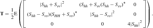
is the surface dielectric constant, and ![]() is a reflection symmetric coherency matrix. Due to the restriction of the model to the first order, roughness and dielectric properties can be easily separated, since roughness only affects the polarimetric span whereas the rest of polarimetric information parameters,
is a reflection symmetric coherency matrix. Due to the restriction of the model to the first order, roughness and dielectric properties can be easily separated, since roughness only affects the polarimetric span whereas the rest of polarimetric information parameters, ![]() in (21.133), depends on the incidence angle and dielectric constant only. At order 1, the cross-polarization is null,
in (21.133), depends on the incidence angle and dielectric constant only. At order 1, the cross-polarization is null, ![]() and the co-polarization channel are perfectly correlated. As a consequence, the entropy of
and the co-polarization channel are perfectly correlated. As a consequence, the entropy of ![]() is very close to 1 and does not fit observations at L or C bands. In order to overcome this limitation, it is proposed in [37] to introduce depolarization within the SPM model by artificially rotating
is very close to 1 and does not fit observations at L or C bands. In order to overcome this limitation, it is proposed in [37] to introduce depolarization within the SPM model by artificially rotating ![]() around the radar line of sight:
around the radar line of sight:
![]() (21.134)
(21.134)
where ![]() is a uniform pdf centered around
is a uniform pdf centered around ![]() and whose width equals
and whose width equals ![]() .
.
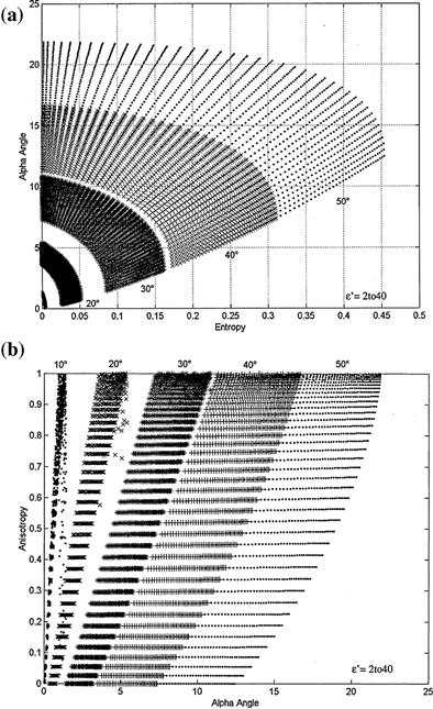
The eigendecomposition of Cloude and Pottier is then applied to ![]() to produce
to produce ![]() . Simulated values presented in Figure 21.41 show that and
. Simulated values presented in Figure 21.41 show that and ![]() may be used to estimate the dielectric constant, whereas the
may be used to estimate the dielectric constant, whereas the ![]() is not correlated with
is not correlated with ![]() . A look-up table procedure is used in [37] to estimate
. A look-up table procedure is used in [37] to estimate ![]() as the value that minimizes the distance between measured and simulated
as the value that minimizes the distance between measured and simulated ![]() values, whereas an empirical relation,
values, whereas an empirical relation, ![]() , is used to estimate the surface roughness. A polynomial relation
, is used to estimate the surface roughness. A polynomial relation ![]() is used to convert dielectric permittivity to volumetric moisture content. Results obtained using L band acquisitions over two sites are given in Figure 21.42.
is used to convert dielectric permittivity to volumetric moisture content. Results obtained using L band acquisitions over two sites are given in Figure 21.42.

2.21.3.5 A method using reflection symmetry and the IEM model
Another technique, introduced in [39,40], proposes an alternative approach, based on the IEM surface scattering model [41] and on the analytical computation of the eigenvalues on a reflection symmetric coherency matrix:
2.21.3.5.1 The SERD and the DERD parameters
Two eigenvalue-based parameters, the Single bounce Eigenvalue Relative Difference (SERD) and the Double bounce Eigenvalue Relative Difference (SERD) have been introduced in [39,40] to characterize natural media. Both parameters are derived from the eigenvalues of a coherency ![]() considering the reflection symmetry hypothesis:
considering the reflection symmetry hypothesis:
 (21.135)
In such a case, it is possible to derive the analytical expressions of the corresponding unsorted (NOS) eigenvalues given by [39,40]:
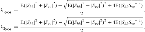 (21.136)
![]()
The first and second eigenvalues depend on the co-polarized backscattering coefficients and on the correlation between the vertical and horizontal channels (![]() ). In this case, the relation
). In this case, the relation ![]() always holds. The third eigenvalue corresponds to cross-polarized channel and is related to multiple scattering for rough surfaces. One may remark that the entropy remains invariant against any permutation within the set of eigenvalues.
always holds. The third eigenvalue corresponds to cross-polarized channel and is related to multiple scattering for rough surfaces. One may remark that the entropy remains invariant against any permutation within the set of eigenvalues.
In order to determine the scattering mechanisms, an analysis is led on the angles extracted from the first two eigenvectors ![]() and
and ![]() , associated to
, associated to ![]() and
and ![]() , respectively. The corresponding
, respectively. The corresponding ![]() angles verify the following property
angles verify the following property
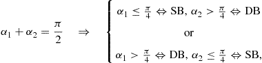 (21.137)
where SB stands for Single Bounce reflection and DB for Double Bounce reflection. The two eigenvalue-based parameters called the Single bounce Eigenvalue Relative Difference (SERD) and the Double bounce Eigenvalue Relative Difference (SERD) are built up to compare the relative importance of the different scattering mechanisms and are defined as:
![]() (21.138)
(21.138)
where ![]() and
and ![]() are the two eigenvalues respectively associated to the single bounce and to the double bounce scattering mechanisms. Due to the lack of sorting, SERD and DERD, cover a wider range than the anisotropy,
are the two eigenvalues respectively associated to the single bounce and to the double bounce scattering mechanisms. Due to the lack of sorting, SERD and DERD, cover a wider range than the anisotropy, ![]() , and are associated to specific scattering mechanisms.
, and are associated to specific scattering mechanisms.
The DERD parameter can be compared with the anisotropy ![]() , whereas the SERD parameter reveals useful with large entropy, in order to determine the nature and the importance of the different scattering mechanisms.
, whereas the SERD parameter reveals useful with large entropy, in order to determine the nature and the importance of the different scattering mechanisms.
2.21.3.5.2 Roughness and moisture retrieval
In order to characterize natural surfaces, the Integral Equation Model (IEM) is employed to derive a polarimetric coherency matrix [39,40]. This model natural accounts for depolarization and produce general reflection symmetric second order representations. Using this model, the DERD parameter can be compared to the polarimetric anisotropy ![]() that is usually employed as a surface roughness descriptor [37]. Figure 21.43 shows, both parameters variations versus the roughness indicator
that is usually employed as a surface roughness descriptor [37]. Figure 21.43 shows, both parameters variations versus the roughness indicator ![]() obtained using the IEM model for various dielectric constants,
obtained using the IEM model for various dielectric constants, ![]() , where k is radar wave number and
, where k is radar wave number and ![]() is the surface root mean square height.
is the surface root mean square height.

The DERD parameter is similar to the anisotropy ![]() for small roughness values, but presents a different behavior for high frequencies. These parameters are very sensitive to surface roughness relative to frequency, whereas the dependence on the dielectric constant
for small roughness values, but presents a different behavior for high frequencies. These parameters are very sensitive to surface roughness relative to frequency, whereas the dependence on the dielectric constant ![]() is less significant. For each dielectric constant
is less significant. For each dielectric constant ![]() value, one anisotropy
value, one anisotropy ![]() value corresponds to two different values of
value corresponds to two different values of ![]() , thus introducing an ambiguity for surface roughness extraction, whereas the DERD is strictly monotonic with
, thus introducing an ambiguity for surface roughness extraction, whereas the DERD is strictly monotonic with ![]() . An important difference between these two parameters is that the dynamic range of the DERD parameter is larger
. An important difference between these two parameters is that the dynamic range of the DERD parameter is larger ![]() than the anisotropy range
than the anisotropy range ![]() . It follows that the DERD parameter has now to be considered as a better surface roughness discriminator. Similar conclusions can be done on indoor measurements realized at the European JRC laboratory [40] and depicted in Figure 21.44.
. It follows that the DERD parameter has now to be considered as a better surface roughness discriminator. Similar conclusions can be done on indoor measurements realized at the European JRC laboratory [40] and depicted in Figure 21.44.
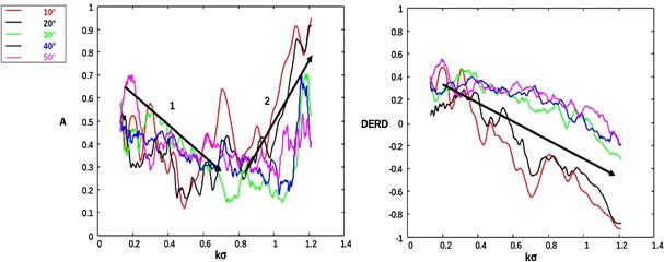
Figure 21.44 Values of A and DERD obtained from data sets acquired by the JRC, for different roughness conditions.
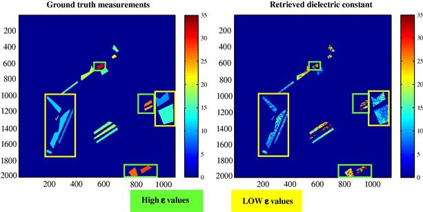
In order to avoid a bias on the mean ![]() [REF] that needs to be compensated using the entropy, only
[REF] that needs to be compensated using the entropy, only ![]() is used to retrieve
is used to retrieve ![]() by comparison with simulated
by comparison with simulated ![]() values. Results obtained over the test site of Alling are shown in Figure 21.45.
values. Results obtained over the test site of Alling are shown in Figure 21.45.
2.21.4 Selected topics in multidimensional polarimetric SAR signal processing
2.21.4.1 Coherent Time-Frequency characterization of complex polarimetric features
Conventional SAR image analysis and geophysical parameter retrieval techniques from strip-map (SAR) data generally assume that scenes are formed of static scatterers observed in the direction perpendicular to the flight track and at a fixed frequency, equal to the emitted signal carrier’s one. When imaging complex objects and media, potential variations of the signal measured during the SAR acquisition may strongly affect feature estimates derived from the resulting SAR data and may lead to erroneous interpretations. It is well known [42] that perturbations induced by the motion of a scatterer may highly modify its SAR response in terms of reflectivity, spatial localization and focusing. Static objects with anisotropic geometrical structures or having a frequency selective response may show a varying electromagnetic behavior as they are illuminated from different positions or at different frequency components during SAR integration. The resulting SAR response being well described by the spatial convolution of an conventional scene SAR image with specific functions accounting for each effect, non ideal features can be easily detected and characterized in the spectral domain.
This section presents different techniques for detecting scatterers having a varying response during the SAR acquisition and characterizing the underlying physical phenomenon that generates these variations. These approaches are based on specific coherent Time-Frequency (TF) decompositions that analyze the response of scatterers by locally estimating the spectral content of their SAR response. These TF techniques can be applied on already focused SAR images and not only on raw SAR signal, and were designed in order to deal with already focused SAR images and not only raw SAR signals and to perform a two-dimensional (2D) rangeazimuth coherent and revertible analysis, i.e., the original SAR image can be reconstructed from local spectral estimates. A physical interpretation of the spectral decomposition in the azimuth and range directions as well as the use of polarimetric SAR data permit to characterize the backscattering properties complex media in a refined way compared to classical techniques and estimate some of their physical features.
2.21.4.1.1 Principles of coherent Time-Frequency analysis of SAR data
2.21.4.1.1.1 SAR image spectral content
As depicted in Figure 21.46, a SAR measurement consists in repeatedly emitting a signal, ![]() , in the across track direction and receiving the echo from the observed scene,
, in the across track direction and receiving the echo from the observed scene, ![]() , at different locations
, at different locations ![]() along the acquisition track. A scatterer
along the acquisition track. A scatterer ![]() located at coordinates
located at coordinates ![]() is observed for different values of the azimuth look angle,
is observed for different values of the azimuth look angle, ![]() , defined by
, defined by ![]() , defined
, defined ![]() being the varying radar-scatterer distance. The range of the azimuth angle is defined by the antenna aperture, whereas the emitted signal is characterized by a bandpass spectrum centered around a carrier frequency
being the varying radar-scatterer distance. The range of the azimuth angle is defined by the antenna aperture, whereas the emitted signal is characterized by a bandpass spectrum centered around a carrier frequency ![]() , with bandwidth
, with bandwidth ![]() .
.
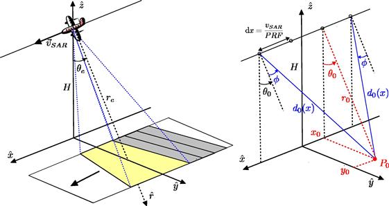
Figure 21.46 Geometrical configuration of a SAR acquisition. Repeated emission-reception of signals, with a rectangular antenna aperture (left). Observation of a scatterer ![]() from different positions along the acquisition track, with corresponding azimuth look angles.
from different positions along the acquisition track, with corresponding azimuth look angles.
After base-band conversion, the received signal can be focused to produce a 2-D coherent image in the azimuth-range domain, ![]() , that represents a reconstruction of the coherent reflectivity of the scene. Under simplifying assumptions and considering ideal acquisition conditions [21], a coherent SAR image may be formulated as convolution of the scene coherent reflectivity,
, that represents a reconstruction of the coherent reflectivity of the scene. Under simplifying assumptions and considering ideal acquisition conditions [21], a coherent SAR image may be formulated as convolution of the scene coherent reflectivity, ![]() and the SAR 2-D impulse response,
and the SAR 2-D impulse response, ![]() and may be represented in both spatial and spectral domains as:
and may be represented in both spatial and spectral domains as:
![]() (21.139)
(21.139)
where ![]() is the 2-D Fourier transform of the SAR image
is the 2-D Fourier transform of the SAR image ![]() and
and ![]() represents the convolution operator. The spectral coordinates
represents the convolution operator. The spectral coordinates ![]() , representing two-way wavenumbers in range and azimuth, are illustrated in Figure 21.47 and can be formulated as [43]:
, representing two-way wavenumbers in range and azimuth, are illustrated in Figure 21.47 and can be formulated as [43]:
![]() (21.140)
(21.140)
where ![]() is the emitted signal wavenumber and can be related to the electrical frequency using,
is the emitted signal wavenumber and can be related to the electrical frequency using, ![]() , through the wave propagation velocity,
, through the wave propagation velocity, ![]() , as
, as ![]() .
.
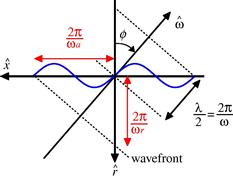
Figure 21.47 Decomposition of a plane wave propagating along ![]() into azimuth and range components. A spherical wave may be represented as a sum of plane waves with varying azimuth orientation
into azimuth and range components. A spherical wave may be represented as a sum of plane waves with varying azimuth orientation ![]() .
.
For an ideal scene, whose reflectivity is uniformly distributed over the spectral domain, the resolutions of the SAR image are driven by the impulse response of the SAR system and are given by
![]() (21.141)
(21.141)
where ![]() stands for the processed azimuthal aperture, whose maximal value is set by the acquisition antenna characteristics.
stands for the processed azimuthal aperture, whose maximal value is set by the acquisition antenna characteristics.
It is worth noting that the direct relation between a SAR image and the reflectivity of scene in (21.139), as well as the physical meaning of the spectral coordinates in (21.140) are valid when dealing with coherent Single Look Complex (SLC) SAR data sets, i.e., each pixel of the SAR image corresponds to a complex number whose modulus is proportional to the focused reflectivity and whose absolute phase depends on the observed medium as well as on the measurement phase history. Transforming an SLC image to an incoherent one, like an intensity image ![]() , involves an irremediable loss of information and interpretation.
, involves an irremediable loss of information and interpretation.
2.21.4.1.1.2 Time frequency decomposition
The T-F decompositions technique selected here is based on the use of a 2-D windowed Fourier transform, or 2-D Gabor transform. This kind of transformation permits to decompose a two-dimensional signal, ![]() , with
, with ![]() a 2-D location, into different spectral components, using a convolution with an analyzing function
a 2-D location, into different spectral components, using a convolution with an analyzing function ![]() , as follows [44]:
, as follows [44]:
![]() (21.142)
(21.142)
where ![]() indicates a position in frequency, and
indicates a position in frequency, and ![]() represents the decomposition result around the spatial and frequency locations
represents the decomposition result around the spatial and frequency locations ![]() and
and ![]() . The application of a Fourier transform to (21.142) shows that the spectrum of
. The application of a Fourier transform to (21.142) shows that the spectrum of ![]() is given by the product of the original signal spectrum and the transform of the analyzing function
is given by the product of the original signal spectrum and the transform of the analyzing function ![]() shifted around the frequency vector
shifted around the frequency vector ![]() :
:
![]() (21.143)
(21.143)
It is clear from Eqs. (21.142) and (21.143) that this time frequency approach may be used to characterize, in the spatial domain, behaviors corresponding to particular spectral components of the signal under analysis, selected by the analyzing function ![]() . Among the wide variety of existing TF analysis methods, the simple atomic decomposition selected in this study presents some interesting properties. It is linear, and hence preserves the coherence and energy of signals, it is not affected by artifacts related to cross-terms and may be inverted, i.e., depending on the analyzing function
. Among the wide variety of existing TF analysis methods, the simple atomic decomposition selected in this study presents some interesting properties. It is linear, and hence preserves the coherence and energy of signals, it is not affected by artifacts related to cross-terms and may be inverted, i.e., depending on the analyzing function ![]() may be reconstructed from a set of TF samples
may be reconstructed from a set of TF samples ![]() , provided that some sampling conditions in spatial and spectral domains are satisfied. The resolutions of the analysis in space and frequency are not independent, and their product is fixed by the Heisenberg-Gabor uncertainty relation, given in 1-D by [44]
, provided that some sampling conditions in spatial and spectral domains are satisfied. The resolutions of the analysis in space and frequency are not independent, and their product is fixed by the Heisenberg-Gabor uncertainty relation, given in 1-D by [44]
![]() (21.144)
(21.144)
This relation specifies that the space-frequency resolution product equals a constant ![]() , determined by
, determined by ![]() . An analyzing function with an excessively narrow spectral bandwidth would involve an excellent spectral resolution but might then lead to a meaningless analysis in the space domain owing to a bad localization, i.e., increasing the description ability of the analysis in one domain worsens its accuracy in the dual one. The nature of the analyzing function is generally chosen so as to preserve resolution while maintaining sufficiently low side-lobe amplitudes in the space domain.
. An analyzing function with an excessively narrow spectral bandwidth would involve an excellent spectral resolution but might then lead to a meaningless analysis in the space domain owing to a bad localization, i.e., increasing the description ability of the analysis in one domain worsens its accuracy in the dual one. The nature of the analyzing function is generally chosen so as to preserve resolution while maintaining sufficiently low side-lobe amplitudes in the space domain.
2.21.4.1.1.3 Time-Frequency decomposition of SAR images
The timefrequency approach presented here deals with processed SAR images, denoted ![]() with
with ![]() , rather than raw data. This type of data is better accessible to common users and is generally processed through compensation procedures to reduce the effects of acquisition errors. In practice the simple SAR image model given in (21.139) needs to be completed in order to account for additional weighting terms, mainly due to the antenna pattern and side-lobe reduction functions, as [45]
, rather than raw data. This type of data is better accessible to common users and is generally processed through compensation procedures to reduce the effects of acquisition errors. In practice the simple SAR image model given in (21.139) needs to be completed in order to account for additional weighting terms, mainly due to the antenna pattern and side-lobe reduction functions, as [45]
![]() (21.145)
(21.145)
with ![]() . The synopsis of the TF decomposition based on the spectral definition on (21.143) is given in Figure 21.48.
. The synopsis of the TF decomposition based on the spectral definition on (21.143) is given in Figure 21.48.
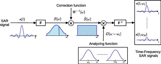
The first step consists of correcting for potential spectral imbalances, represented by ![]() in Eq. (21.145), in the original, full-resolution SAR image. This can be achieved by calculating average image spectra in range and azimuth and then multiplying the full-resolution spectrum
in Eq. (21.145), in the original, full-resolution SAR image. This can be achieved by calculating average image spectra in range and azimuth and then multiplying the full-resolution spectrum ![]() by the inverse of the estimated 2-D weighting function. The TF decomposition is then conducted by multiplying the corrected spectrum by the Fourier transform of the analyzing function and going back to the spatial domain. The resulting still focused SAR image
by the inverse of the estimated 2-D weighting function. The TF decomposition is then conducted by multiplying the corrected spectrum by the Fourier transform of the analyzing function and going back to the spatial domain. The resulting still focused SAR image ![]() has a lower resolution than the original SAR data and depicts the scene behavior over the 2D frequency domain located in the neighborhood of
has a lower resolution than the original SAR data and depicts the scene behavior over the 2D frequency domain located in the neighborhood of ![]() . As it might be observed in (21.145), the use of processed data limits the spectral exploration range to the one of the reference function used for raw data processing and focusing. In order to emphasize the physical interpretation of coherent SAR image analysis, one may simplify the wavenumber expressions given in (21.140) using narrow beamwidth and bandwidth approximations
. As it might be observed in (21.145), the use of processed data limits the spectral exploration range to the one of the reference function used for raw data processing and focusing. In order to emphasize the physical interpretation of coherent SAR image analysis, one may simplify the wavenumber expressions given in (21.140) using narrow beamwidth and bandwidth approximations
![]() (21.146)
(21.146)
Time-Frequency decomposition in the azimuth direction consists of deriving a set of images containing different parts of the SAR Doppler spectrum with a reduced resolution, but corresponding to different azimuth look angles. This kind of analysis can be applied to detect objects or media with anisotropic behaviors, like scatterers with complex geometrical structures, human- made objects, or natural media having periodic structures in the case of agricultural areas, or linear alignments of strong scatterers [45]. In the range direction, TF analysis permits to compare the response of a scene observed at different frequencies, contained within the emitted signal spectral domain, and can be used to detect and characterize media with frequency-sensitive responses, like resonating spherical or cylindrical objects, periodic structures, or coupled scatterers with interfering characteristics.
Polarimetric SLC SAR images can be easily decomposed by applying the presented approach independently over each polarization channel. Usual polarimetric representations may then be reconstructed to study the polarimetric behavior of a scene around specific spectral locations.
 (21.147)
where spatial locations, ![]() , have been omitted.
, have been omitted.
2.21.4.1.2 Characterization of natural environments with non-stationary polarimetric SAR responses
2.21.4.1.2.1 Discrimination of non-stationary POLSAR responses
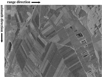
Discrete Time-Frequency decomposition in range and azimuth. As shown in (21.147), the timefrequency decomposition can be applied around any frequency location inscribed within the rangeazimuth frequency range defined by the SAR transfer function ![]() . Nevertheless, it is often useful to first process the analysis around a limited (discrete) set of frequency locations to appreciate the global behavior of the scene under observation and emphasize changes from one subspectral image to another by minimizing their correlation, The polarimetric SAR data set under study has been acquired by the DLR E-SAR sensor, at L band, over the Alling test site in Germany. The original image resolution is 2 m in range and 1 m in azimuth, corresponding to an azimuthal variation of the look angle of approximately
. Nevertheless, it is often useful to first process the analysis around a limited (discrete) set of frequency locations to appreciate the global behavior of the scene under observation and emphasize changes from one subspectral image to another by minimizing their correlation, The polarimetric SAR data set under study has been acquired by the DLR E-SAR sensor, at L band, over the Alling test site in Germany. The original image resolution is 2 m in range and 1 m in azimuth, corresponding to an azimuthal variation of the look angle of approximately ![]() and a chirp bandwidth of 75 MHz. Figure 21.49 shows the full- resolution span image corresponding to the total polarimetric backscattered power. The considered scene is mainly composed of agricultural fields and forest. An urban area is located at the bottom left corner of the image.
and a chirp bandwidth of 75 MHz. Figure 21.49 shows the full- resolution span image corresponding to the total polarimetric backscattered power. The considered scene is mainly composed of agricultural fields and forest. An urban area is located at the bottom left corner of the image.
The decomposition in the azimuth direction is performed using independent subspectra and keeping the range resolution to its original value. Figure 21.50 shows results obtained over an area corresponding to plowed fields. Images of the span, H, and ![]() parameters are represented for different azimuthal look angles and for the full-resolution case. It can be observed in Figure 21.50 that large variations in the scattering mechanism nature,
parameters are represented for different azimuthal look angles and for the full-resolution case. It can be observed in Figure 21.50 that large variations in the scattering mechanism nature, ![]() , and degree of randomness, H, occur while the azimuth look angle changes. For particular azimuth look angles, some fields show a sudden change of behavior: the span reaches a maximum value, whereas the polarimetric indicators H and
, and degree of randomness, H, occur while the azimuth look angle changes. For particular azimuth look angles, some fields show a sudden change of behavior: the span reaches a maximum value, whereas the polarimetric indicators H and ![]() are characterized by low values. The stripes in the span image, indicating that coherent constructive and destructive interferences occur within the pixels, are characteristic for Bragg resonant scattering over periodic surfaces [45].
are characterized by low values. The stripes in the span image, indicating that coherent constructive and destructive interferences occur within the pixels, are characteristic for Bragg resonant scattering over periodic surfaces [45].

Figure 21.50 Polarimetric parameters at full resolution (center) and after 1-D TF analysis in the azimuth (left) and range (right) directions.
Other types of media may also have nonstationary polarimetric features during the azimuthal integration. It was observed that some point targets and linear structures, such as diffracting edges or road berms, have significant backscattering pattern variations as the look angle changes. In particular, metallic link fencing was found to present a scattering mechanism ranging from single-bounce up to double-bounce scattering, depending on the SAR azimuthal look angle. In general, nonstationary targets have strongly anisotropic shapes, or facets acting like directional scatterers, involving changes in the underlying scattering mechanism and in the total backscattered power.
In contrast, forested areas have a stationary behavior during the SAR integration. Backscattering from forested areas at L band is known to be dominated by volume diffusion, which corresponds to the scattering over randomly distributed anisotropic constituents. The coherent integration of the randomly scattered waves leads to a response that is characterized by a high intensity and low degree of polarization, but with isotropic behavior.
Detection of non-stationary polarimetric TF behaviors. Each pixel of the SAR scene is associated with a set of R independent target vectors, ![]() with
with ![]() , derived from independent range-azimuth subspectra, i.e., subspectra selected using non-overlapping functions
, derived from independent range-azimuth subspectra, i.e., subspectra selected using non-overlapping functions ![]() . Under the classical speckle affected scattering hypothesis, these target vectors follow independent complex Gaussian multivariate distributions,
. Under the classical speckle affected scattering hypothesis, these target vectors follow independent complex Gaussian multivariate distributions, ![]() . The stationary aspect of the scattering behavior of each pixel may then be studied by comparing the second order statistics of
. The stationary aspect of the scattering behavior of each pixel may then be studied by comparing the second order statistics of ![]() for different spectral locations, i.e., by testing the following hypothesis:
for different spectral locations, i.e., by testing the following hypothesis:
![]() (21.148)
(21.148)
As it is shown in [46] this hypothesis can be tested easily using sample coherency matrices obtained from ![]() independent realizations or looks of each TF target vector,
independent realizations or looks of each TF target vector, ![]() :
:
 (21.149)
The TF stationary behavior of ![]() is evaluated by means of a Maximum Likelihood (ML) ratio,
is evaluated by means of a Maximum Likelihood (ML) ratio, ![]() , built from the R independent sample coherency matrices as follows:
, built from the R independent sample coherency matrices as follows:
![]() (21.150)
(21.150)
Replacing the likelihoods in (21.150) by their expression and the expectations by their ML estimates, on gets the following simple expression [45]
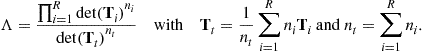 (21.151)
The hypothesis is accepted and the pixel under test is considered to have a stationary polarimetric TF behavior, with an arbitrarily chosen probability of false alarm ![]() , if
, if ![]() , where the relation between the threshold value and the probability of false alarm,
, where the relation between the threshold value and the probability of false alarm, ![]() , has been derived in [45]. The ML ratio and nonstationary pixel map shown in Figure 21.51 indicate that an important number of pixels have a nonstationary behavior during the duration of the SAR acquisition. Most of the varying scatterers belong to agricultural fields affected by Bragg resonance. Complex targets and diffracting edges, whose scattering characteristics highly depend on the observation position, are discriminated over built-up areas and linear alignment of scatterers.
, has been derived in [45]. The ML ratio and nonstationary pixel map shown in Figure 21.51 indicate that an important number of pixels have a nonstationary behavior during the duration of the SAR acquisition. Most of the varying scatterers belong to agricultural fields affected by Bragg resonance. Complex targets and diffracting edges, whose scattering characteristics highly depend on the observation position, are discriminated over built-up areas and linear alignment of scatterers.
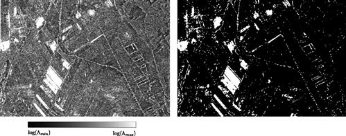
Figure 21.51 Discrimination of non-stationary scatterers. Image of the ML ratio in log-scale (left), non-stationary pixel map (right). Non stationary pixels are represented in white (For interpretation of the references to color in this figure legend, the reader is referred to the web version of this book.).
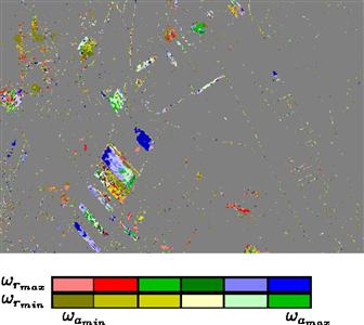
The ML ratio based detection approach may be further developed to determine nonstationary scattering behavior position in the range Doppler spectrum by comparing the contributions of each subspectrum image in the global ML ratio information [45]. It can be observed from the localization results displayed in Figure 21.52 on many fields affected by Bragg resonance that some groups of pixels, belonging to the same field, have a maximum anisotropic behavior in different subapertures. This is a consequence of the sliding effects of Bragg resonance on periodic structures, that is described in the next section.
2.21.4.1.2.2 Analysis of Bragg resonant scattering over natural soils using a polarimetric 2-D TF continuous decomposition
In the scene under examination, Bragg resonance over agricultural fields is an important source of polarimetric variations. Bragg resonance is due to the coherent summation of simultaneously constructive contributions from a set of scatterers and is likely to happen during the observation of periodic surfaces or randomly irregular surfaces with a strong periodic component, as described in 1-D in Figure 21.53 A random surface, ![]() , with a quasi-periodic component in the
, with a quasi-periodic component in the ![]() direction, can be described as
direction, can be described as
![]() (21.152)
(21.152)
where ![]() and
and ![]() are the spatial period and amplitude, respectively, of the periodic component of
are the spatial period and amplitude, respectively, of the periodic component of ![]() , and the random perturbation term,
, and the random perturbation term, ![]() , corresponds to an isotropic stationary random rough surface. This component is fully described by
, corresponds to an isotropic stationary random rough surface. This component is fully described by ![]() , the standard deviation of its zero mean Gaussian height probability density function, and
, the standard deviation of its zero mean Gaussian height probability density function, and ![]() , its correlation function. The Bragg resonance condition can be written as a function of the incident wavelength,
, its correlation function. The Bragg resonance condition can be written as a function of the incident wavelength, ![]() , as
, as
![]() (21.153)
(21.153)
where ![]() corresponds to the local amplitude of the ground wave vector at the,
corresponds to the local amplitude of the ground wave vector at the, ![]() is an unknown integer number indicating the mode of the resonance,
is an unknown integer number indicating the mode of the resonance, ![]() is the local angle of incidence and
is the local angle of incidence and ![]() the azimuthal angular difference between the observation position and the normal to the rows of the periodic surface. In the case of SAR measurements,
the azimuthal angular difference between the observation position and the normal to the rows of the periodic surface. In the case of SAR measurements, ![]() can be decomposed as
can be decomposed as ![]() , where
, where ![]() represents the orientation of the surface with respect to the normal to the SAR platform flight track, and
represents the orientation of the surface with respect to the normal to the SAR platform flight track, and ![]() with the angle of observation in the azimuthal spectrum, as defined in (21.140). Yueh et al. [47] developed several approaches to model the scattering of electromagnetic waves from randomly perturbed periodic surfaces. Their study reports that the influence of the resonating modes on the total backscattering response varies significantly with the surface parameters. As it can be seen in Figure 21.53, for a large surface correlation length,
with the angle of observation in the azimuthal spectrum, as defined in (21.140). Yueh et al. [47] developed several approaches to model the scattering of electromagnetic waves from randomly perturbed periodic surfaces. Their study reports that the influence of the resonating modes on the total backscattering response varies significantly with the surface parameters. As it can be seen in Figure 21.53, for a large surface correlation length, ![]() , and for low values of the azimuth orientation angle,
, and for low values of the azimuth orientation angle, ![]() , almost all the intensity peaks corresponding to different resonance modes can be discriminated. As
, almost all the intensity peaks corresponding to different resonance modes can be discriminated. As ![]() increases, the scattering pattern becomes smoother and only a few dominant resonance peaks can be observed. In the presence of resonance, the co-polarization returns
increases, the scattering pattern becomes smoother and only a few dominant resonance peaks can be observed. In the presence of resonance, the co-polarization returns ![]() and
and ![]() have almost identical values, characterized by a high intensity. As the resonant effect decreases, i.e., for high values of
have almost identical values, characterized by a high intensity. As the resonant effect decreases, i.e., for high values of ![]() , these polarimetric channels have distinct responses, with a significantly reduced amplitude. According to the resonance condition enounced in (21.153) similar anisotropic fields with different locations in range,
, these polarimetric channels have distinct responses, with a significantly reduced amplitude. According to the resonance condition enounced in (21.153) similar anisotropic fields with different locations in range, ![]() , or differently oriented, i.e., with different
, or differently oriented, i.e., with different ![]() values may resonate at different azimuthal frequencies. If the resonance conditions cannot be satisfied for any azimuthal angle within the antenna aperture or if the surface scattering characteristics do not show a resonance peak, they also might not resonate at all [48].
values may resonate at different azimuthal frequencies. If the resonance conditions cannot be satisfied for any azimuthal angle within the antenna aperture or if the surface scattering characteristics do not show a resonance peak, they also might not resonate at all [48].
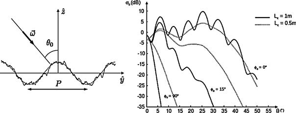
Figure 21.53 Example of randomly perturbed periodic surface (left) and its associated backscattering coefficient, at L-band, with ![]() , and
, and ![]() .
.
Moreover, some fields may have parts resonating at different positions in the azimuthal frequency domain due to the joint dependence of the resonance condition on the incidence and azimuth angles, as seen in (21.153). This phenomenon is illustrated in Figure 21.54, where the location of a resonance peak is plotted as a function of the range and azimuth frequencies. As the azimuthal look angle, ![]() , varies, the set of incidence angles
, varies, the set of incidence angles ![]() satisfying Eq. (21.153) changes, leading to the apparition of sliding resonating stripes in the
satisfying Eq. (21.153) changes, leading to the apparition of sliding resonating stripes in the ![]() . The width of the resonating stripes is fixed by the width of the analyzing function in the azimuth and range directions,
. The width of the resonating stripes is fixed by the width of the analyzing function in the azimuth and range directions, ![]() or equivalently
or equivalently ![]() .
.
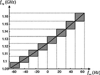
Figure 21.54 Location of resonance peaks in the ![]() plane. The solid line indicates the location of a resonance peak for a periodic surface characterized by P = 0.6 m and observed at L band. Gray areas indicate the location of potential resonance areas for each range-azimuth sub-spectrum.
plane. The solid line indicates the location of a resonance peak for a periodic surface characterized by P = 0.6 m and observed at L band. Gray areas indicate the location of potential resonance areas for each range-azimuth sub-spectrum.
A range-azimuth continuous Time-Frequency analysis is performed over three points ![]() , located at different range positions inside a plowed field [48]. As depicted in Figure 21.55, results can be represented, for each point, in the rangeazimuth frequency plane. The results of the timefrequency analysis, as shown in Figure 21.55, demonstrate that all three points under investigation do not have a stationary range and azimuth scattering behavior. Some
, located at different range positions inside a plowed field [48]. As depicted in Figure 21.55, results can be represented, for each point, in the rangeazimuth frequency plane. The results of the timefrequency analysis, as shown in Figure 21.55, demonstrate that all three points under investigation do not have a stationary range and azimuth scattering behavior. Some ![]() couples show high span values corresponding to low
couples show high span values corresponding to low ![]() and
and ![]() . These observations agree with the predictions of the scattering model developed by Yueh et al. [47]. As the surface resonates, the co-polarization signals tend to be similar, involving a low
. These observations agree with the predictions of the scattering model developed by Yueh et al. [47]. As the surface resonates, the co-polarization signals tend to be similar, involving a low ![]() value, typical for surface reflection. This scattering mechanism is weighted by a strong intensity and dominates secondary intensities, potentially corresponding to multiple scattering terms, and results in a very low entropy value. This nonstationary behavior was found to have a preponderant influence on the polarimetric properties of resonating field at full resolution. Here,
value, typical for surface reflection. This scattering mechanism is weighted by a strong intensity and dominates secondary intensities, potentially corresponding to multiple scattering terms, and results in a very low entropy value. This nonstationary behavior was found to have a preponderant influence on the polarimetric properties of resonating field at full resolution. Here, ![]() and
and ![]() values are significantly lower than those for similar fields that remained unaffected by Bragg resonance. The oblique resonating stripes, shown in the different range frequency planes in Figure 21.55, illustrate well the dependence of the resonance condition on both range and azimuth frequencies, as shown in Figure 21.54.
values are significantly lower than those for similar fields that remained unaffected by Bragg resonance. The oblique resonating stripes, shown in the different range frequency planes in Figure 21.55, illustrate well the dependence of the resonance condition on both range and azimuth frequencies, as shown in Figure 21.54.
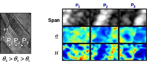
Figure 21.55 Location of test points ![]() ,
, ![]() , and
, and ![]() and range azimuth frequency representation plane (left) and representation of polarimetric characteristics in this domain.
and range azimuth frequency representation plane (left) and representation of polarimetric characteristics in this domain.
It can also be observed that as the incidence angle increases, from ![]() to
to ![]() , the oblique resonating stripe slides from low azimuth frequencies to higher ones. This displacement of the resonance locations is due to the dependence of the Bragg condition on the incidence angle and corroborates the analysis of the Bragg resonance as presented in Figure 21.54. Polarimetric indicators of pixels that do not belong to resonating stripes are unaffected by the Bragg resonance and have values similar to those observed over stationary fields.
, the oblique resonating stripe slides from low azimuth frequencies to higher ones. This displacement of the resonance locations is due to the dependence of the Bragg condition on the incidence angle and corroborates the analysis of the Bragg resonance as presented in Figure 21.54. Polarimetric indicators of pixels that do not belong to resonating stripes are unaffected by the Bragg resonance and have values similar to those observed over stationary fields.
2.21.4.1.3 TF polarimetric characterization of specific scatterers
2.21.4.1.3.1 Detection of point-like scatterers using the Internal Hermitian Product (IHP)
This approach, developed by Souyris et al. [49], was the first of a series or works on coherent TF analysis that fully exploit the physical nature of SAR signal together with polarimetric diversity. Its objective is to assess the joint use of the magnitude and the phase of a SAR polarimetric image for point target detection and analysis. The detection principle is based on the fact that scattering by point like scatterers is a coherent process, i.e., during the SAR integration waves follow a specular path. Their T-F response, after an adequate phase compensation should ideally be constant, in practice remain coherent. Over speckle affected environments, scattering is due to wave diffusion by a large number of scatterers in a random and spatially uncorrelated way. In consequence their spectral response should show a low level of correlation.
Single polarization IHP. A natural way to detect the presence of a correlated signal, i.e., a target, embedded in uncorrelated noise, i.e., the clutter, is to compute the normalized correlation between two samples:
 (21.154)
In an ideal configuration, ![]() , where
, where ![]() represents the ideally constant target response and
represents the ideally constant target response and ![]() the uncorrelated clutter contribution
the uncorrelated clutter contribution ![]() if the samples originate from independent spectra. In this case the TF normalized correlation writes
if the samples originate from independent spectra. In this case the TF normalized correlation writes
![]() (21.155)
(21.155)
where it was assumed that the variance of the clutter response ![]() was constant over the spectral domain. The correlation is than a function of the Signal to Clutter power Ratio (SCR), i.e., when a coherent object with a strong responses is illuminated, it can be detected by thresholding
was constant over the spectral domain. The correlation is than a function of the Signal to Clutter power Ratio (SCR), i.e., when a coherent object with a strong responses is illuminated, it can be detected by thresholding ![]() . As reported in [49], such an approach may lead to poor result if the SCR is not high enough and another approach is proposed, based on the IHP, defined as
. As reported in [49], such an approach may lead to poor result if the SCR is not high enough and another approach is proposed, based on the IHP, defined as
![]() (21.156)
(21.156)
It is simply the un-normalized correlation between two signal samples. As it is shown on Figure 21.56 this approach permits to improve the contrast between a target and its background. One may argue that such an approach may be more associated to strong scatterer selection, based on their TF coherence properties, rather than detection, since the amplitude IHP is not normalized.
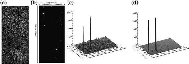
Figure 21.56 (a) original L-band SAR image acquired by the ONERA/RAMSES sensor at L band, (b) 2-look IHP image, and (c) 3-D view of the upper part of the image, (d) 3-D view of the upper part of the IHP image. From [49].
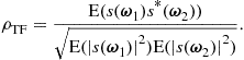
Polarimetric IHP. The IHP concept is exported to the polarimetric case [49] using the definition of the polarimetric correlation used in polarimetric SAR interferometry (POL-inSAR) [15]
![]() (21.157)
(21.157)
where ![]() ,
, ![]() and
and ![]() is a projection unitary vector that permits to select one or a linear combination of polarization channels. This vector is then tuned over the space of unitary 3-element complex vectors to find the optimal value,
is a projection unitary vector that permits to select one or a linear combination of polarization channels. This vector is then tuned over the space of unitary 3-element complex vectors to find the optimal value, ![]() , that maximizes
, that maximizes ![]() . The polarimetric properties of the target response are then given by
. The polarimetric properties of the target response are then given by ![]() that may be processed through classical decomposition techniques to obtain specific polarimetric indicators. An example of application to polarimetric SAR data is given in Figure 21.57.
that may be processed through classical decomposition techniques to obtain specific polarimetric indicators. An example of application to polarimetric SAR data is given in Figure 21.57.
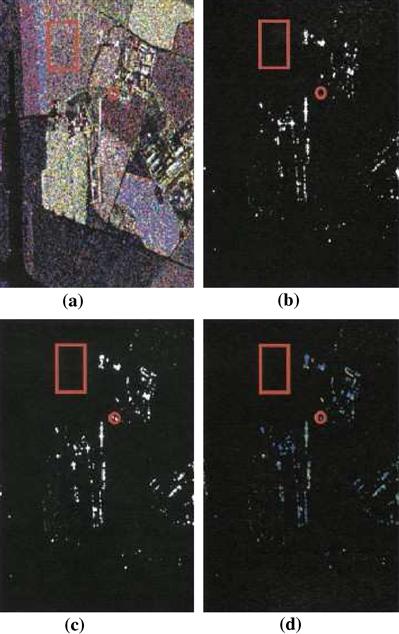
Figure 21.57 Polarimetric 2L-IHP. (Red circle) Test over point targets. (Red square) Test over speckle. (a) ONERA/RAMSES polarimetric SAR scene (5-m resolution, L-band) Red is HH. Green is HV. Blue is VV. (b) 2L-IHP, polarization HH. (c) POL-2L-IHP of the SAR scene. (d) Detected target analysis. Red indicates a dominant odd number of reflections. Green a dipole-like scattering. Blue a dominant double-bounce effects. From [49] (For interpretation of the references to color in this figure legend, the reader is referred to the web version of this book.).
2.21.4.1.3.2 Detection of coherent scatterers and their polarimetric characteristics
Persistent Scatterers (PS), whose response remain constant along time, are of particular interest for differential interferometry applications to subsidence monitoring [50]. Since it is likely that scatterers having stable TF responses, i.e., when observed from different positions and different frequencies, remain stable in time too, studies were led to investigate which types of constructions or objects actually behave as Coherent Scatterers.
2.21.4.1.3.3 CS detection based on TF entropy
In [51] the normalized correlation approach of (21.154) is compared to a new stability indicator, the TF entropy, ![]() . Unlike (21.154), this indicator can handle more than two samples at a time. The signal of a given polarization channel is sampled at
. Unlike (21.154), this indicator can handle more than two samples at a time. The signal of a given polarization channel is sampled at ![]() different spectral locations, over independent or slightly overlapping spectral domains to create a TF signal vector,
different spectral locations, over independent or slightly overlapping spectral domains to create a TF signal vector, ![]() and estimate its
and estimate its ![]() covariance matrix,
covariance matrix, ![]() :
:
![]() (21.158)
(21.158)
Similarly to the single-image polarimetric case, a TF entropy can be computed as [51]
 (21.159)
where ![]() is the
is the ![]() eigenvalue of
eigenvalue of ![]() . If different TF samples are maximally correlated, the TF entropy equals
. If different TF samples are maximally correlated, the TF entropy equals ![]() , whereas for totally uncorrelated signals having the same amplitude,
, whereas for totally uncorrelated signals having the same amplitude, ![]() tends toward
tends toward ![]() . The analysis conducted over the city of Dresden indicates that many CS can be found over all the polarimetric channels (Figures 21.58 and 21.59). In the central part of the image is located the city center of Dresden, whereas in the central upper part a park with forested and vegetated areas can be recognized. Note that individual buildings and building blocks oriented parallel to the azimuth direction are characterized by a strong dihedral component, while buildings/blocks that have an orientation angle with respect to azimuth flight direction are characterized by a strong cross-polarized scattering component. One may note the position of the CSs in the region of the park (in the walking promenades and on the central place within the park) and in the dense urbanized areas (on the corners of buildings, along the streets, and on the two bridges over the Elbe River).
. The analysis conducted over the city of Dresden indicates that many CS can be found over all the polarimetric channels (Figures 21.58 and 21.59). In the central part of the image is located the city center of Dresden, whereas in the central upper part a park with forested and vegetated areas can be recognized. Note that individual buildings and building blocks oriented parallel to the azimuth direction are characterized by a strong dihedral component, while buildings/blocks that have an orientation angle with respect to azimuth flight direction are characterized by a strong cross-polarized scattering component. One may note the position of the CSs in the region of the park (in the walking promenades and on the central place within the park) and in the dense urbanized areas (on the corners of buildings, along the streets, and on the two bridges over the Elbe River).

Figure 21.58 (a) Color-coded polarimetric image of Dresden. (b) Detected coherent scatterers (in red) in HH polarization, superimposed to the intensity image. From [51] (For interpretation of the references to color in this figure legend, the reader is referred to the web version of this book.).

Figure 21.59 (Left) Detected CSs in lexicographic polarimetric basis. (Central upper) Details of the park region. (Central lower) Details of a dense urban area. (Right upper) Ikonos image of the Groer Garten Park. (Right lower) Ikonos image of the dense urban area. From [51].
The detected CS are characterized, in general, by high amplitudes, and low polarimetric entropy values. Their majority has a man-made character, a fact that predicts a relative high temporal stability. Because of their strong polarized behavior polarimetric acquisition diversity increases significantly the performance of CSs detection. Indeed for the Dresden data set the number of detected CSs by using fully polarimetric data, and an optimization similar to (21.157), is by a factor up to ten higher compared to the number of CSs detected by using single-polarization data. The fact that the majority of the CSs is not depolarizing, and can be described by its scattering matrix, makes polarimetric information essential for the characterization, interpretation, and information extraction from individual CSs [51].
2.21.4.1.3.4 CS detection based on multiple criteria
In [52], a study of High Resolution X-band images is conducted over urban structures. The stability of the TF responses using a feature vector containing the coefficient of variation of the signal intensity, the TF entropy and gradient-based indicators of the stability of the continuous TF response. A statistical analysis of this feature vector is led to discriminate scatters having a coherent or unstable behavior in frequency, in azimuth or in both directions. A polarimetric analysis is led over specific objects. At such a high resolution, the TF behavior of objects could be used for their recognition using automatic techniques. An illustration is given in Figure 21.60.
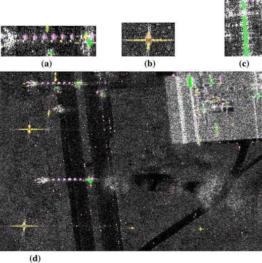
Figure 21.60 Examples of target point classification. Resolution 10 cm. (Red) Frequency invariant. (Purple) Range variant. (Green) Azimuth variant. (Gray levels) 2-D variant. (a) Resonant in range (ladder). (b) Frequency invariant (trihedral). (c) Azimuth variant (building corner). (d) Classification on the entire scene. From [52] (For interpretation of the references to color in this figure legend, the reader is referred to the web version of this book.).
2.21.4.1.4 Polarimetric Time-Frequency characterization of a dense urban area
2.21.4.1.4.1 Polarimetric Time-Frequency features
Figure 21.61 shows a color-coded polarimetric SAR image of the city of Dresden acquired by DLR’s E-SAR sensor data at L-band. The scene is mainly composed of built-up areas including vegetation spots. A forest and a park can be seen on the left part of the image and a river with smooth banks is located on the right part.
Polarimetric properties of media are generally investigated through a decomposition of second order multivariate polarimetric representations. The resulting parameters provide information on the media geometrical structure and on the underlying scattering mechanisms. Two parameters, obtained from the well known eigenvector-based decomposition introduced in [13] are displayed in Figure 21.62.
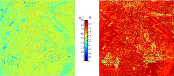
The entropy image shown in Figure 21.62 reveals that the polarimetric behavior of most of the scene is highly random. Over urban areas, the polarimetric response is composed of a large number of different polarimetric contributions originating from complex building structures as wall as from surrounding vegetation. The resulting high entropy involves that an interpretation of polarimetric indicators may not be relevant. Over buildings aligned with the flight track direction, the entropy has intermediate values and the ![]() parameter reveals the presence of dominant single and double bounce reflexions. Buildings which do not face the radar track are characterized by a strong cross-polarization component and high entropy and can hardly be discriminated from vegetated areas.
parameter reveals the presence of dominant single and double bounce reflexions. Buildings which do not face the radar track are characterized by a strong cross-polarization component and high entropy and can hardly be discriminated from vegetated areas.
Figure 21.63 presents a continuous TF analysis in the azimuth direction of three different media: a building facing the radar, an oriented building, and a forested area. The SPAN, corresponding to the sum of the intensities in all polarimetric channels, and the polarimetric ![]() angle are computed for the different media at each frequency location and mean values are then estimated over pixels belonging to the object.
angle are computed for the different media at each frequency location and mean values are then estimated over pixels belonging to the object.
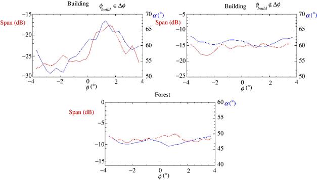
Figure 21.63 Continuous TF analysis in the azimuth direction (SPAN in red, ![]() in blue) (For interpretation of the references to color in this figure legend, the reader is referred to the web version of this book.).
in blue) (For interpretation of the references to color in this figure legend, the reader is referred to the web version of this book.).
A non stationary behavior is clearly visible in Figure 21.63 with a sudden a large variation of both SPAN and ![]() levels with the observation angle in azimuth
levels with the observation angle in azimuth ![]() . This anisotropic behavior is due to the highly directional patterns of coherent scattering mechanisms which may occur as the radar faces a large artificial structure, such as a building [53]. This particular effect can only be observed if the building orientation with respect to the radar flight track falls within the processed antenna azimuth aperture.
. This anisotropic behavior is due to the highly directional patterns of coherent scattering mechanisms which may occur as the radar faces a large artificial structure, such as a building [53]. This particular effect can only be observed if the building orientation with respect to the radar flight track falls within the processed antenna azimuth aperture.
On the contrary, oriented buildings and vegetated areas, like forest patches, show stationary behaviors. The identification of buildings from their TF response thus requires an additional criterion to complement the stationarity information. It is known that man-made objects are likely to have a coherent response, whereas natural media may be considered as random. The discrimination of such responses can be achieved by studying the coherence of the backscattered polarimetric signal in the Time-Frequency domain and requires the use of an adequate TF polarimetric SAR (PolSAR) signal model.
2.21.4.1.4.2 PolSAR TF signal modeling and analysis
PolSAR data TF model. The proposed TF signal model [54] is given by the following expression, where the spatial coordinates, ![]() , have be omitted:
, have be omitted:
![]() (21.160)
(21.160)
The signal ![]() contains the full coherent polarimetric polarization information and can be associated to a well-known scattering vector [13]:
contains the full coherent polarimetric polarization information and can be associated to a well-known scattering vector [13]:
![]() (21.161)
(21.161)
where ![]() represents an element of the
represents an element of the ![]() scattering matrix
scattering matrix ![]() sampled at the frequency coordinates
sampled at the frequency coordinates ![]() .
.
The signal described in (21.160) is composed of two contributions:
• The term ![]() is highly coherent and can be associated to a deterministic or almost deterministic target response. Depending on the structure of the observed object, the response can remain constant during the SAR acquisition, or can be non-stationary if the backscattering behavior is sensitive to the azimuth angle of observation or illumination frequency.
is highly coherent and can be associated to a deterministic or almost deterministic target response. Depending on the structure of the observed object, the response can remain constant during the SAR acquisition, or can be non-stationary if the backscattering behavior is sensitive to the azimuth angle of observation or illumination frequency.
• The second term, ![]() , represents the response of distributed environments. It is uncorrelated, but may follow a non-stationary behavior in particular cases, e.g., vegetated terrains with a strong topography, very dense environments whose response results from the sum of a large number of uncorrelated contributions.
, represents the response of distributed environments. It is uncorrelated, but may follow a non-stationary behavior in particular cases, e.g., vegetated terrains with a strong topography, very dense environments whose response results from the sum of a large number of uncorrelated contributions.
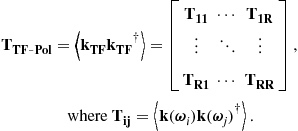
This composite model may be tested using ![]() second order statistics:
second order statistics:
• The coherence of ![]() can be used to determine the dominant component within the pixel under consideration. A high value indicates that
can be used to determine the dominant component within the pixel under consideration. A high value indicates that ![]() is the most important term in (21.160), and a low one corresponds to scattering from an incoherent, distributed, medium.
is the most important term in (21.160), and a low one corresponds to scattering from an incoherent, distributed, medium.
• The stability of the dominant component can then be tested by studying the stationarity of the variance of ![]() .
.
Second order statistics. Due to the signal high dimensionality, usual scalar tools are not well adapted to the study of second-order TF polarimetric statistics. A polarimetric TF target vector is built by gathering the PolSAR information sampled at ![]() spectral coordinates
spectral coordinates ![]() .
.
![]() (21.162)
(21.162)
The sampling coordinates, ![]() , and the frequency domain resolution of the analyzing function
, and the frequency domain resolution of the analyzing function ![]() are chosen so that the
are chosen so that the ![]() sub-spectra do not overlap and span the whole full resolution spectrum [48]. A polarimetric TF sample covariance matrix,
sub-spectra do not overlap and span the whole full resolution spectrum [48]. A polarimetric TF sample covariance matrix, ![]() , is then computed as follows
, is then computed as follows
 (21.163)
Non-stationary pixel discrimination. Stationarity is assessed by testing the fluctuations of the variance of the signal at the different spectral locations [46,48]. In the polarimetric case, the signal sample variance is given by a ![]() polarimetric coherency matrix, i.e., by the diagonal terms of the
polarimetric coherency matrix, i.e., by the diagonal terms of the ![]() matrix:
matrix: ![]() . The polarimetric TF response is considered as stationary if the sample
. The polarimetric TF response is considered as stationary if the sample ![]() matrices, assumed to follow independent complex Wishart distributions
matrices, assumed to follow independent complex Wishart distributions ![]() with
with ![]() looks, have the same expectation
looks, have the same expectation ![]() . The corresponding hypothesis is given by:
. The corresponding hypothesis is given by:
![]() (21.164)
(21.164)
The corresponding Maximum Likelihood (ML) ratio is:
![]() (21.165)
(21.165)
The likelihood terms in (21.165) are maximized by replacing the expectation matrices by the ML estimates and the hypothesis is tested using the resulting ML test [45], which takes the following form:
![]() (21.166)
(21.166)
Figure 21.64 presents a log-image of the ![]() parameter on the Dresden test site, obtained with four spectral coordinates in the azimuth direction over the Dresden test site.
parameter on the Dresden test site, obtained with four spectral coordinates in the azimuth direction over the Dresden test site.
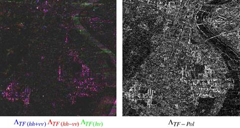
Figure 21.64 Non stationary TF behavior indicator, ![]() , computed separately for different polarimetric channels (left) simultaneously using the whole polarimetric information (right).
, computed separately for different polarimetric channels (left) simultaneously using the whole polarimetric information (right).
The ![]() parameter reach high values over natural areas indicating a stationary spectral behavior. Over buildings,
parameter reach high values over natural areas indicating a stationary spectral behavior. Over buildings, ![]() decreases, pointing out the invalidity of the stationary hypothesis over such objects. Highly anisotropic pixels, such as those corresponding to the wall-ground dihedral reflection or specular reflection from oriented roofs are clearly identified in Figure 21.64 due to their very low stationary aspect.
decreases, pointing out the invalidity of the stationary hypothesis over such objects. Highly anisotropic pixels, such as those corresponding to the wall-ground dihedral reflection or specular reflection from oriented roofs are clearly identified in Figure 21.64 due to their very low stationary aspect.
Coherent pixel discrimination. In [51], the eigenvalues of a single-polarization covariance matrix have been used to derive a coherency indicator. These eigenvalues carry information on the correlation structure, but are also sensitive to potential PolSAR fluctuations due to non-stationarity. A solution has been proposed in order to overcome this limitation and to jointly use all the polarimetric channels [54]. Under the hypothesis of uncorrelated spectral responses, the off-diagonal terms of the TF covariance matrix verify:
![]() (21.167)
(21.167)
The corresponding ML ratio is given by:
![]() (21.168)
(21.168)
This ML ratio expression can be rewritten as:
![]() (21.169)
(21.169)
with
 (21.170)
![]()
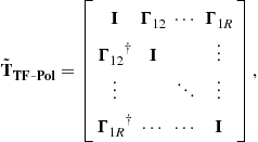
The normalized covariance matrix, ![]() results from the whitening of the TF polarimetric covariance matrix by the separate polarimetric information at each frequency location. This representation is then insensitive to spectral polarimetric intensity variations and is characterized by its off-diagonal matrices
results from the whitening of the TF polarimetric covariance matrix by the separate polarimetric information at each frequency location. This representation is then insensitive to spectral polarimetric intensity variations and is characterized by its off-diagonal matrices ![]() which can be viewed as an extension of the scalar normalized correlation coefficient to the polarimetric case. The ML ratio in (21.168) is a function of the eigenvalues of
which can be viewed as an extension of the scalar normalized correlation coefficient to the polarimetric case. The ML ratio in (21.168) is a function of the eigenvalues of ![]() , which reflect the correlation structure: flat for decorrelated responses (
, which reflect the correlation structure: flat for decorrelated responses (![]() ), heterogeneous for correlated ones. Taking into account
), heterogeneous for correlated ones. Taking into account ![]() peculiar form, a correlation indicator, named TF-Pol coherence, can be defined as [54]:
peculiar form, a correlation indicator, named TF-Pol coherence, can be defined as [54]:
![]() (21.171)
(21.171)
Figure 21.65 presents an image of ![]() over the Dresden test site, computed from four spectral locations in the azimuth direction.
over the Dresden test site, computed from four spectral locations in the azimuth direction.

Figure 21.65 TF coherence indicator, ![]() , computed separately for different polarimetric channels (left) simultaneously using the whole polarimetric information (right).
, computed separately for different polarimetric channels (left) simultaneously using the whole polarimetric information (right).
As expected, the TF-Pol coherence is high over buildings due to the presence of strong coherent reflectors. It can be also noticed that buildings are identified independently of their orientation.
2.21.4.1.4.3 PolSAR TF analysis
PolSAR TF classification. The stationarity and coherence indicators derived above can be merged to classify the scene. Both ![]() and
and ![]() parameters are thresholded and combined into four classes. The application of the fusion strategy over the Dresden site is shown in Figure 21.66.
parameters are thresholded and combined into four classes. The application of the fusion strategy over the Dresden site is shown in Figure 21.66.

Figure 21.66 TF polarimetric classification. Classification scheme (left) results obtained over Dresden (right).
The resulting map permits a good estimation of building locations. A physical interpretation can be given for each of the four classes:
• Coherent and stationary pixels (white class): The ![]() term in (21.160) is dominant and constant during the SAR acquisition. This kind of behavior corresponds to strong scatterers with an isotropic response, like oriented buildings, lamp-posts, ….
term in (21.160) is dominant and constant during the SAR acquisition. This kind of behavior corresponds to strong scatterers with an isotropic response, like oriented buildings, lamp-posts, ….
• Coherent and non stationary pixels (yellow class): The ![]() contribution dominates but varies during the measure, causing fluctuation of the signal with the azimuth angle of observation. This anisotropic effect is characteristic of buildings facing the radar track, whose response is affected by a strong and highly directive pattern, mainly due double bounce reflections or specular single bounce reflection over roofs tilted toward the radar.
contribution dominates but varies during the measure, causing fluctuation of the signal with the azimuth angle of observation. This anisotropic effect is characteristic of buildings facing the radar track, whose response is affected by a strong and highly directive pattern, mainly due double bounce reflections or specular single bounce reflection over roofs tilted toward the radar.
• Incoherent and stationarity pixels (green class): The uncorrelated component ![]() dominates and has stable second order statistics. This class corresponds to natural environments (forests, fields, grass areas, …) of distributed artificial media such as roads, roof tops, terraces, …
dominates and has stable second order statistics. This class corresponds to natural environments (forests, fields, grass areas, …) of distributed artificial media such as roads, roof tops, terraces, …
• Incoherent and non-stationary pixels (red class): This class indicates the presence of complex scattering contributions, which change during the SAR integration, and sum-up in an incoherent way, like in layover areas.
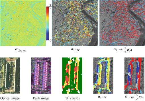
TF cleaning of PolSAR data. As it was shown in Figure 21.62, the full resolution PolSAR information can hardly be used to analyze the scene geophysical properties due to a very high entropy inherent to the study of dense environments. The proposed PolSAR TF analysis technique can also be used to improve in a significant way the interpretation of polarimetric indicators. The most coherent TF scattering mechanisms is described by the first eigenvector of ![]() , which can be transformed back to the H-V polarimetric basis using a matrix
, which can be transformed back to the H-V polarimetric basis using a matrix ![]() , satisfying
, satisfying ![]() . From this eigenvector, one can extract an
. From this eigenvector, one can extract an ![]() parameter which shows a much more contrasted and relevant information than the original full resolution parameter
parameter which shows a much more contrasted and relevant information than the original full resolution parameter ![]() . Figure 21.67 shows different images of a building of the scene. A comparison between the T-F classification results and the optical image reveals that both the double bounce reflexion is considered as a non-stationary and coherent scattering mechanism, whereas the roof layover is seen as non-stationary and uncorrelated, due to the superposition of the roof and ground contributions. A thresholding of
. Figure 21.67 shows different images of a building of the scene. A comparison between the T-F classification results and the optical image reveals that both the double bounce reflexion is considered as a non-stationary and coherent scattering mechanism, whereas the roof layover is seen as non-stationary and uncorrelated, due to the superposition of the roof and ground contributions. A thresholding of ![]() with respect to
with respect to ![]() , permits to easily separate these two different mechanisms and could be used to get a rough estimate of the building height. Such an information might be useful to interferometric phase unwrapping algorithms which generally face ambiguity issues over urban areas.
, permits to easily separate these two different mechanisms and could be used to get a rough estimate of the building height. Such an information might be useful to interferometric phase unwrapping algorithms which generally face ambiguity issues over urban areas.
2.21.4.2 Analysis of volumetric media using polarimetric SAR interferometry
2.21.4.2.1 A brief introduction to SAR interferometry
2.21.4.2.1.1 Relation between interferometric phase and the height of a scatterer
The geometrical configuration of an interferometric acquisition, depicted in Figure 21.68, shows two sensors, located at slightly different positions, that measure the coherent SAR response of a scatterer. The relative positions of the sensors is measured by the baseline ![]() and the angle
and the angle ![]() . After focusing of the SAR signals and co-registration of the SAR images, the response of the scatterer is given by
. After focusing of the SAR signals and co-registration of the SAR images, the response of the scatterer is given by
![]() (21.172)
(21.172)
where ![]() represents the absolute and unknown phase of the reponse of each object. For a small baseline and if the acquisitions are made within a sufficiently short amount of time, the amplitude and phase of the object responses may be considered identical,
represents the absolute and unknown phase of the reponse of each object. For a small baseline and if the acquisitions are made within a sufficiently short amount of time, the amplitude and phase of the object responses may be considered identical, ![]() . In this case, the interferometric phase difference, or interferogram, is given by
. In this case, the interferometric phase difference, or interferogram, is given by
![]() (21.173)
(21.173)
This interferometric phase being proportional to the path difference, ![]() , it is sensitive to both the elevation of the scatterer with respect to a reference plane and to the range distance
, it is sensitive to both the elevation of the scatterer with respect to a reference plane and to the range distance ![]() . A local linearization permits to isolate the elevation-dependent part
. A local linearization permits to isolate the elevation-dependent part ![]() :
:
![]() (21.174)
(21.174)
where ![]() can be computed from the geometrical configuration and hence compensated and
can be computed from the geometrical configuration and hence compensated and ![]() is given by
is given by
![]() (21.175)
(21.175)
One may note that the estimation of the interferometric phase as the argument of a complex exponential may imply a wrapping due to the limited domain of definition of the ![]() operator. As a consequence
operator. As a consequence
![]() (21.176)
(21.176)
This ambiguity can generally be overcome using phase unwrapping techniques.
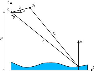
2.21.4.2.1.2 Interferometric coherence
Over homogeneous distributed environments, the acquired are random variables whose statistics may be studied using the 2-element vector, ![]() , following a complex normal distribution,
, following a complex normal distribution, ![]() , where the covariance matrix
, where the covariance matrix ![]() may be written as
may be written as
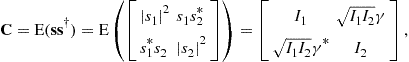 (21.177)
where
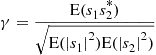 (21.178)
is called the interferometric coherence and may be used to estimate the interferometric phase ![]() . Using
. Using ![]() independent realizations, or looks, of
independent realizations, or looks, of ![]() , ML estimates may be computed as [21,22]
, ML estimates may be computed as [21,22]
 (21.179)
In addition to the need of a large number of looks, ![]() , a good estimate of the interferometric phase requires a large value of the modulus of the coherence, since
, a good estimate of the interferometric phase requires a large value of the modulus of the coherence, since ![]() when
when ![]() and
and ![]() reaches a maximum as
reaches a maximum as ![]() .
.
The coherence may be modeled as a product of a large number of contributions, as, for instance:
![]() (21.180)
(21.180)
Each element represent a potential source of decorrelation between the acquired signals, due to the presence of additive noise, errors during the acquisition, processing and referencing of the signals, to changes of the scenes between the acquisitions, to spectral shifts induced by acquisition geometry and to vertical decorrelation induced by the presence of a volumic medium. Very few of these can be compensated a posteriori and each of them may influence the phase estimation accuracy since
![]() (21.181)
(21.181)
2.21.4.2.1.3 The random volume over ground model for a single polarization channel
The last term of the coherence decomposition in (21.180) is related to the structure of the observed medium through an integral relation [15,55–58]
 (21.182)
where ![]() represents the equivalent density of coherent reflectivity in the elevation direction. The interferometric coherence may then be used to guess some characteristics of the vertical structure of the observed volume, provided that the other terms in (21.180) are known or compensated. In order to estimate the possibilities of such an approach, one may use a simple model of a homogeneous Random semi-transparent Volume lying over a Ground consisting of a rough surface, the RVOG model, depicted in Figure 21.69[56,58].
represents the equivalent density of coherent reflectivity in the elevation direction. The interferometric coherence may then be used to guess some characteristics of the vertical structure of the observed volume, provided that the other terms in (21.180) are known or compensated. In order to estimate the possibilities of such an approach, one may use a simple model of a homogeneous Random semi-transparent Volume lying over a Ground consisting of a rough surface, the RVOG model, depicted in Figure 21.69[56,58].
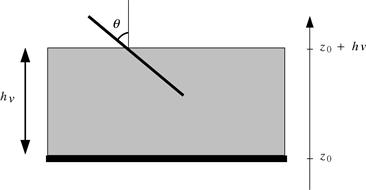
The volume is assumed to be made of particles having the same reflectivity ![]() and the same constant extinction properties. i.e.,
and the same constant extinction properties. i.e.,
![]() (21.183)
(21.183)
then
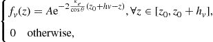 (21.184)
where the factor ![]() account for round-trip attenuation. The ground reflectivity distribution is then given by
account for round-trip attenuation. The ground reflectivity distribution is then given by
![]() (21.185)
(21.185)
The intensities backscattered by the ground and the volume are given by
![]() (21.186)
(21.186)
The general unresolved expression of the coherence is then
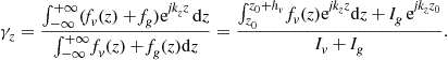 (21.187)
In order to provide a physical interpretation for expression (21.187), cases with different levels of complexity can be investigated.
Case 0: Transparent volume. In this extremely simple case, the volume response is null, i.e., ![]() . The coherence
. The coherence
![]() (21.188)
(21.188)
has a unitary modulus and its argument provides the elevation of the ground.
Case 1: Lossless volume and no ground. The extinction of waves when they travel through the volume is null, ![]() and the ground reflectivity is null,
and the ground reflectivity is null, ![]() . In this case
. In this case ![]() represents the coherence behavior of the volume only
represents the coherence behavior of the volume only
![]() (21.189)
(21.189)
The coherence argument indicates exactly the absolute elevation of the center of the volume, whereas its modulus depends on its width ![]() . This case is illustrated in Figure 21.70.
. This case is illustrated in Figure 21.70.
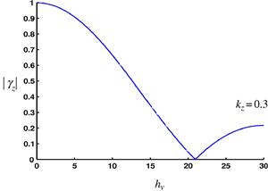
Case 2: Volume with constant linear extinction and no ground. The extinction ![]() is constant over the volume and the ground reflectivity is null,
is constant over the volume and the ground reflectivity is null, ![]() . The expression of the coherence is
. The expression of the coherence is
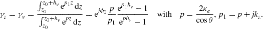 (21.190)
The magnitude and phase behaviors of ![]() are illustrated in Figure 21.71 for different values of extinction. For a quasi-null extinction, the coherence magnitude has a sinc-like shape and the phase center is located at the center of the volume. As the extinction increases, the magnitude pattern becomes flatter and close to
are illustrated in Figure 21.71 for different values of extinction. For a quasi-null extinction, the coherence magnitude has a sinc-like shape and the phase center is located at the center of the volume. As the extinction increases, the magnitude pattern becomes flatter and close to ![]()
![]() when
when ![]() is large. The phase center moves then towards the higher interface of the volume. This behavior is due to the fact that as
is large. The phase center moves then towards the higher interface of the volume. This behavior is due to the fact that as ![]() increases the wave penetration depth inside the volume decreases and the particles that participate more to the scattering phenomenon are those located near the upper interface. For reduced penetration depths, the decorrelation induced by the numerator of (21.190) becomes negligible.
increases the wave penetration depth inside the volume decreases and the particles that participate more to the scattering phenomenon are those located near the upper interface. For reduced penetration depths, the decorrelation induced by the numerator of (21.190) becomes negligible.
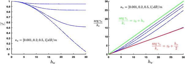
Case 3: Volume with constant linear extinction and ground. The extinction ![]() is constant over the volume and the ground reflectivity is non null. The expression of the coherence is [55,56,58]
is constant over the volume and the ground reflectivity is non null. The expression of the coherence is [55,56,58]
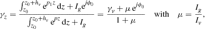 (21.191)
where ![]() , called the ground to volume intensity ratio, can be considered as a key parameter of the RVOG coherence which steers the coherence
, called the ground to volume intensity ratio, can be considered as a key parameter of the RVOG coherence which steers the coherence ![]() between to extreme behaviors,
between to extreme behaviors, ![]() for
for ![]() and
and ![]()
![]() . For intermediate values a single coherence term is not sufficient for analyzing the RVOG model.
. For intermediate values a single coherence term is not sufficient for analyzing the RVOG model.
2.21.4.2.2 Pol-inSAR representations
Polarimetric and interferometric signals consist of two polarimetric target vectors, ![]() , acquired from slightly different positions. As it has been mentioned for polarimetric TF signal processing, the computation of the correlation between multivariate signals requires to use projectors. The Pol-inSAR coherence has then been defined by Cloude and Papathanassiou as:
, acquired from slightly different positions. As it has been mentioned for polarimetric TF signal processing, the computation of the correlation between multivariate signals requires to use projectors. The Pol-inSAR coherence has then been defined by Cloude and Papathanassiou as:
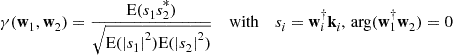 (21.192)
and ![]() is a projection unitary vector that permits to select one or a linear combination of polarization channels. This coherence can be obtained from the
is a projection unitary vector that permits to select one or a linear combination of polarization channels. This coherence can be obtained from the ![]() POL-inSAR coherency matrix, defined as:
POL-inSAR coherency matrix, defined as:
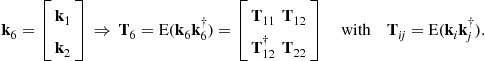 (21.193)
The coherence can then be expressed as
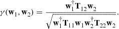 (21.194)
Cloude and Papthanassiou have found the projections defining the optimal scattering mechanisms that maximize ![]() [15]. Nevertheless using different projection vectors
[15]. Nevertheless using different projection vectors ![]() is, in general not recommended. Indeed the phase and magnitude of coherences computed between different polarimetric channels depend on the interferometric configuration, but also on the polarimetric correlation within each separate image. In general, the POL-inSAR coherence is simplified to
is, in general not recommended. Indeed the phase and magnitude of coherences computed between different polarimetric channels depend on the interferometric configuration, but also on the polarimetric correlation within each separate image. In general, the POL-inSAR coherence is simplified to
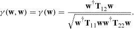 (21.195)
2.21.4.2.3 Polarimetric RVOG model
The principles of a polarimetric solution to the RVOG model are given in Figure 21.72.
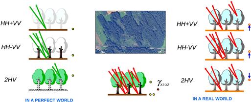
Figure 21.72 Ideal and realistic scattering configuration over a volumetric natural environment (Courtesy of Dr. Kostas Papthanassiou).
The objective is to isolate specific polarimetric scattering mechanisms ![]() and
and ![]() that null
that null ![]() or
or ![]() , respectively. In an ideal world,
, respectively. In an ideal world, ![]() and
and ![]() , and a priori knowledge on the domain of variation of
, and a priori knowledge on the domain of variation of ![]() permits to estimate
permits to estimate ![]() with a reasonable precision. In general, such RVOG polarimetric eigen-mechanisms do not exist, i.e.,
with a reasonable precision. In general, such RVOG polarimetric eigen-mechanisms do not exist, i.e., ![]() . An original solution, proposed in [58], is summarized in the following. It is based on the hypothesis that the reflectivity and extinction within the volume do not depend on polarization:
. An original solution, proposed in [58], is summarized in the following. It is based on the hypothesis that the reflectivity and extinction within the volume do not depend on polarization:
![]() (21.196)
(21.196)
This hypothesis correspond to a azimuthal symmetric form for the coherency matrix an is then reasonable for a dense volume of uniformly oriented particles. Under this hypothesis, the only polarization-dependent parameter is the response of the ground ![]() . The polarimeric version of the coherence given in (21.191) can be expressed as:
. The polarimeric version of the coherence given in (21.191) can be expressed as:
![]() (21.197)
(21.197)
This relation can be written under the following form
![]() (21.198)
(21.198)
which is the parametric equation of a line segment, between ![]() and
and ![]() in the complex plane. This means that when the RVOG model is valid, complex coherences obtained for arbitrary polarimetric projection vectors are located on a line segment in the complex plane, as illustrated on Figure 21.73.
in the complex plane. This means that when the RVOG model is valid, complex coherences obtained for arbitrary polarimetric projection vectors are located on a line segment in the complex plane, as illustrated on Figure 21.73.
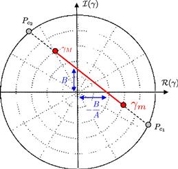
2.21.4.2.4 Estimation of the height of a RVOG using POL-inSAR data
2.21.4.2.4.1 Vegetation bias removal
In practice the ground to volume intensity ratio ![]() never reaches the limits of its domain of definition
never reaches the limits of its domain of definition ![]() , i.e.,
, i.e., ![]() . For a ground contribution with a sufficiently low entropy, there exist a scattering mechanism, typically HV, so that
. For a ground contribution with a sufficiently low entropy, there exist a scattering mechanism, typically HV, so that ![]() and in this case
and in this case ![]() . Due to the lack of polarization selectivity of volume scattering, the extremity of the line segment corresponding to
. Due to the lack of polarization selectivity of volume scattering, the extremity of the line segment corresponding to ![]() cannot be used to estimate the ground elevation. Cloude and Papathanassiou proposed to overcome this problem by extrapolating the line segment until it intercepts the unitary circle, since the RVOG model for a transparent medium,
cannot be used to estimate the ground elevation. Cloude and Papathanassiou proposed to overcome this problem by extrapolating the line segment until it intercepts the unitary circle, since the RVOG model for a transparent medium, ![]() . This physical interpretation permits to reduce an important elevation bias linked with the completely depolarized volume response.
. This physical interpretation permits to reduce an important elevation bias linked with the completely depolarized volume response.
2.21.4.2.4.2 Practical vegetation height estimation
In [55], Cloude proposes a theoretically sub-optimal but practically robust method to estimate the height of a volume from POL-inSAR data sets.
Line segment. From a L-look sample Pol-inSAR coherency matrix, estimate the line parameters, e.g., ![]() and
and ![]() in Figure 21.73. It is recommended to use the analytical expressions provided in [59] instead of a least-square fit based on sample coherences generated from (21.195) and a set of pre-defined or random projection vectors. Indeed the approach in [59] is immediate and corresponds to the generation of an infinite number of coherences.
in Figure 21.73. It is recommended to use the analytical expressions provided in [59] instead of a least-square fit based on sample coherences generated from (21.195) and a set of pre-defined or random projection vectors. Indeed the approach in [59] is immediate and corresponds to the generation of an infinite number of coherences.
Volume and ground coherences. This can be done by selecting one of the segment extremity ![]() and
and ![]() as
as ![]() , e.g., one may chose the one closer to
, e.g., one may chose the one closer to ![]() . Extrapolate the other extremity of the segment to the unitary circle in order to determine
. Extrapolate the other extremity of the segment to the unitary circle in order to determine ![]() .
.
Estimate the height assuming an infinite extinction. As mentioned earlier, for an infinite extinction value, the phase center of ![]() correspond to the upper interface of the volume. Then
correspond to the upper interface of the volume. Then
![]() (21.199)
(21.199)
It is unlikely that ![]() , so
, so ![]() will indeed correspond to a phase center located within the volume. This value might underestimate the true volume height.
will indeed correspond to a phase center located within the volume. This value might underestimate the true volume height.
Estimate the height assuming an null extinction. For a null extinction, the volume coherence magnitude as a sinc-like shape. The corresponding height might be estimated as
![]() (21.200)
(21.200)
It is also unlikely that ![]() , i.e., that the phase center is at its lowest possible elevation. This value might underestimate the true volume height.
, i.e., that the phase center is at its lowest possible elevation. This value might underestimate the true volume height.
Empirical linear combination. The final height estimate is
![]() (21.201)
(21.201)
Recommended ![]() value: 0.4
value: 0.4
This semi-empirical approach reveals more robust than a theoretically more correct one, since it combines uses separate estimates based on the modulus and phase of ![]() , linearly combines estimates with opposed biases and does not use numerical values of the extinction that main cause severe artifacts. Examples of results obtained over forested areas using polarimetric and interferometric SAR processing are given in Figures 21.74 and 21.75.
, linearly combines estimates with opposed biases and does not use numerical values of the extinction that main cause severe artifacts. Examples of results obtained over forested areas using polarimetric and interferometric SAR processing are given in Figures 21.74 and 21.75.
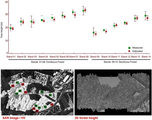
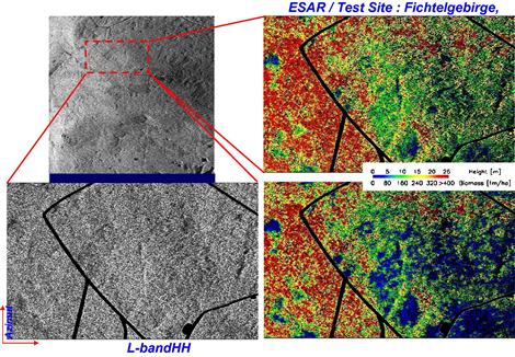
2.21.4.3 Analysis of volumetric media using polarimetric SAR tomography
2.21.4.3.1 Basics of SAR Tomographic imaging
SAR tomographic imaging, using Multi-Baseline Interferometry (MB-InSAR), is based on the acquisition of ![]() SAR signals along slightly shifted trajectories
SAR signals along slightly shifted trajectories ![]() , as illustrated on Figure 21.76. Each pair of trajectories is separated by a baseline. After focusing, compensating and georeferencing the acquired signals,
, as illustrated on Figure 21.76. Each pair of trajectories is separated by a baseline. After focusing, compensating and georeferencing the acquired signals, ![]() 2-D SAR images are obtained,
2-D SAR images are obtained, ![]() , where
, where ![]() represents the azimuth location and
represents the azimuth location and ![]() , the proximal distance of a given point.
, the proximal distance of a given point.
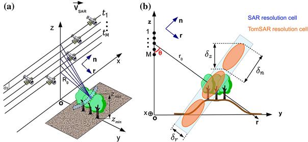
Figure 21.76 Geometrical configuration of an MB-InSAR measurement (a), SAR and TomSAR resolutions cells (b).
As shown on Figure 21.76, due to its intrinsic cylindrical ambiguity, classical 2-D SAR imaging is not well adapted to the characterization of volumic media. For a given focusing position ![]() , the focused SAR results from the coherent integration of the reflectivity density
, the focused SAR results from the coherent integration of the reflectivity density ![]() of the considered medium.
of the considered medium.
![]() (21.202)
(21.202)
where ![]() represents one resolution cell with a cylindrical slice layer shape, whose upper and lower limits are defined by the observed volumic media. The resolution cell limits are given by:
represents one resolution cell with a cylindrical slice layer shape, whose upper and lower limits are defined by the observed volumic media. The resolution cell limits are given by:
![]() (21.203)
(21.203)
with ![]() and
and ![]() the SAR resolution in azimuth and distance respectively.
the SAR resolution in azimuth and distance respectively.
The formulation in (21.202) assumes that ![]() is is a function of the elevation position only, i.e.,
is is a function of the elevation position only, i.e., ![]() and
and ![]() are have sufficiently low values and variations in these directions within a resolution cell may be neglected. The vertical wavenumber,
are have sufficiently low values and variations in these directions within a resolution cell may be neglected. The vertical wavenumber, ![]() accounts for variations of the interferometric phase from one image to the other and can be calculated from the geometric configuration of the acquisition. The purpose of Tomographic SAR (TomSAR) imaging, illustrated on Figure 21.76, is to improve the vertical resolution of the SAR measurement in order to estimate the volumic density of the reflectivity
accounts for variations of the interferometric phase from one image to the other and can be calculated from the geometric configuration of the acquisition. The purpose of Tomographic SAR (TomSAR) imaging, illustrated on Figure 21.76, is to improve the vertical resolution of the SAR measurement in order to estimate the volumic density of the reflectivity ![]() in a more accurate way. To do so, the
in a more accurate way. To do so, the ![]() acquired SAR signals
acquired SAR signals ![]() , obtained for different numbers of vertical waves
, obtained for different numbers of vertical waves ![]() are used in the frame of a classical problem of spectral estimation, for which a series of solutions can be applied [60,61]. Using Multi-Baseline Polarimetric Interferometry (MB-PolInSAR), Polarimetric Tomographic SAR (PolTomSAR) imaging can provide the observed medium more precise localization and more detailed physical features. The first airborne TOMSAR experiment was conducted by the DLR using their ESAR sensor at L band over the test site of Oberpfaffenhofen [62]. The data set consist of 14 SAR images acquired over quasi-parallel tracks within a short period of time. This study revealed the fantastic power analysis of the combination of 3-D imaging with SAR. Some results of this work are presented in Figure 21.76 where it is shown that tomography can be used to reliably locate scatterers in elevation, estimate building heights and image forest canopies. Tomograms performed over different polarimetric channels can be combined to appreciate the 3-D polarimetric behavior of the media under observation.
are used in the frame of a classical problem of spectral estimation, for which a series of solutions can be applied [60,61]. Using Multi-Baseline Polarimetric Interferometry (MB-PolInSAR), Polarimetric Tomographic SAR (PolTomSAR) imaging can provide the observed medium more precise localization and more detailed physical features. The first airborne TOMSAR experiment was conducted by the DLR using their ESAR sensor at L band over the test site of Oberpfaffenhofen [62]. The data set consist of 14 SAR images acquired over quasi-parallel tracks within a short period of time. This study revealed the fantastic power analysis of the combination of 3-D imaging with SAR. Some results of this work are presented in Figure 21.76 where it is shown that tomography can be used to reliably locate scatterers in elevation, estimate building heights and image forest canopies. Tomograms performed over different polarimetric channels can be combined to appreciate the 3-D polarimetric behavior of the media under observation.
Recently, other studies were performed to characterized natural volumetric media, i.e., forested areas, using SAR tomography combined with polarization diversity [63–65]. Similarly to the RVOG model mentioned above, the POLTOMSAR reponse of a forest is assumed to be made of two main components related to the ground and volume contribution. A specific Kronecker structure is then used to extract the vertical and polarimetric features of both components from a set of polarimetric images. Despite its mathematical exactness, the estimated components are affected by an ambiguity and several solutions are possible. Fortunately, both the spatial and polarimetric domains covered by these possible solutions shrinks considerably as the number of images increases, i.e., as vertical resolution improves. One may note that this ambiguous aspect is common to all POL-inSAR techniques for such an application. Examples of tomograms obtained over volumetric environments are shown in Figures 21.77 and 21.78.
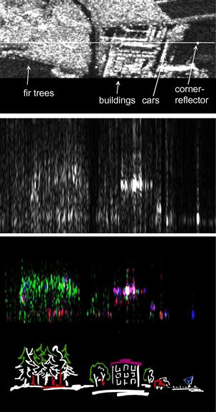
Figure 21.77 First airborne tomographic SAR experiment: HH SAR image at L band of the DLR buildings and surroundings (top) HH intensity tomogram estimated over a linear path indicated on the SAR image (middle) Color coded tomogram obtained from estimates performed over the Pauli basis polarimetric channels (bottom). Courtesy of Dr. Andreas Reigber.
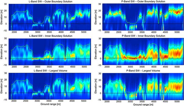
Figure 21.78 Polarimetric SAR tomograms of a boreal forest performed at L (left) and P (right) over data acquired by the DLR within the BioSAR campaign. From top to bottom are represented different solutions that all fit very well with the H100 height obtained through LIDAR measurements and denoted by the green line. Courtesy of Dr. Stefano Tebaldini.
2.21.4.3.2 Tomographic signal models
2.21.4.3.2.1 TomSAR signal models
Considering an azimuth-range resolution cell that contains ![]() backscattering contributions from scatterers located at different heights and assuming no decorrelation between the different acquisitions, the received data vector,
backscattering contributions from scatterers located at different heights and assuming no decorrelation between the different acquisitions, the received data vector, ![]() , can be formulated as follows:
, can be formulated as follows:
 (21.204)
where ![]() indicates one of the
indicates one of the ![]() independent realizations of the signal acquisition, also called looks. The source signal vector,
independent realizations of the signal acquisition, also called looks. The source signal vector, ![]() , contains the unknown complex reflection coefficient of the
, contains the unknown complex reflection coefficient of the ![]() scatterers, and
scatterers, and ![]() represents the complex additive noise, assumed to be Gaussianly distributed with zero mean variance
represents the complex additive noise, assumed to be Gaussianly distributed with zero mean variance ![]() , and to be white in time and space with, i.e.,
, and to be white in time and space with, i.e., ![]() and
and ![]() . The steering vector
. The steering vector ![]() contains the interferometric phase information associated to a source located at the elevation position
contains the interferometric phase information associated to a source located at the elevation position ![]() above the reference focusing plane and is given by:
above the reference focusing plane and is given by:
![]() (21.205)
(21.205)
where ![]() is the two-way vertical wavenumber between the master and the
is the two-way vertical wavenumber between the master and the ![]() th acquisition tracks. The corresponding perpendicular baseline
th acquisition tracks. The corresponding perpendicular baseline ![]() is aligned with the cross-range direction. The carrier wavelength is represented by
is aligned with the cross-range direction. The carrier wavelength is represented by ![]() , whereas
, whereas ![]() stands for the incidence angle and
stands for the incidence angle and ![]() is the slant range distance between the master track and the scatterer. The steering matrix
is the slant range distance between the master track and the scatterer. The steering matrix ![]() consists of
consists of ![]() steering vectors corresponding each to a backscattering source:
steering vectors corresponding each to a backscattering source:
![]() (21.206)
(21.206)
with ![]() , the vector of unknown source heights.
, the vector of unknown source heights.
Considering now interferometric decorrelation between different acquisitions, the initial model in (21.204) may be reformulated as a sum of contributions from random sources [60]:
 (21.207)
where ![]() accounts for both the reflection coefficient of the
accounts for both the reflection coefficient of the ![]() th source,
th source,![]() and its potential variations between the interferometric acquisitions or over the
and its potential variations between the interferometric acquisitions or over the ![]() realizations. Depending on the type of scatterer under observation, the source signal
realizations. Depending on the type of scatterer under observation, the source signal ![]() possesses varying statistical properties. The resulting composite signal
possesses varying statistical properties. The resulting composite signal ![]() may then follow different scattering behaviors [66].
may then follow different scattering behaviors [66].
• Distributed scatterers: The media are characterized by a scattering response having a random behavior conferred by the speckle effect. Under some assumptions summarized in [67]. the scattered signal may be modeled using a multiplicative random term following a centered complex gaussian distribution with unitary variance
![]() (21.208)
(21.208)
where ![]() represents the multiplicative speckle term and
represents the multiplicative speckle term and ![]() is the complex response of the
is the complex response of the ![]() th scatterer, its reflectivity being given by
th scatterer, its reflectivity being given by ![]() . The
. The ![]() covariance matrix
covariance matrix ![]() describes the interferometric coherence and, for a well calibrated acquisition system, contains unitary diagonal elements, whereas off-diagonal terms depend on the acquisition conditions This kind of source signal is well adapted to the modeling of scattering over natural environments, like rough surfaces, ground and volumetric environments.
describes the interferometric coherence and, for a well calibrated acquisition system, contains unitary diagonal elements, whereas off-diagonal terms depend on the acquisition conditions This kind of source signal is well adapted to the modeling of scattering over natural environments, like rough surfaces, ground and volumetric environments.
• Deterministic scatterers: The backscattered source signal is frozen over all the observations and presents no decorrelation between the different acquisitions. For a well calibrated system, its form is given by
![]() (21.209)
(21.209)
This behavior is generally related to specular scattering mechanisms and can be observed over coherent scatterers like calibrators, facets facing the radar, double-bounce reflections over dihedral-like objects having smooth surfaces (like ground-trunk interactions and double bounce reflections between an object and the ground), or may be linked to resonant behaviors over quasi-periodic media [48].
• Hybrid scatterers: Consist of a mixture of coherent and distributed scatterers [48]. In such cases, a hybrid MB-InSAR signal model, introduced by Sauer et al. [68], may be used to describe the received signal, as it includes both deterministic and distributed contributions:
 (21.210)
This type of signals can be frequently encountered when dealing with intermediate-resolution SAR images.
2.21.4.3.2.2 PolTomSAR signal model
The polarimetric response of a scatterer is fully described by its (![]() ) complex scattering matrix
) complex scattering matrix ![]() . The scattering matrix can be vectorized using, for instance, the Pauli basis matrix set
. The scattering matrix can be vectorized using, for instance, the Pauli basis matrix set ![]() [12], in order to build a target vector
[12], in order to build a target vector ![]()
![]() (21.211)
(21.211)
where ![]() represents the polarimetric span [12] of the scatterer response, and
represents the polarimetric span [12] of the scatterer response, and ![]() represents a unitary polarimetric target vector, i.e.,
represents a unitary polarimetric target vector, i.e., ![]() . In an MB-PolInSAR configuration, the array response may be represented by re-arranging the
. In an MB-PolInSAR configuration, the array response may be represented by re-arranging the ![]() acquired polarimetric signals,
acquired polarimetric signals, ![]() with
with ![]() the track index, under the form of a
the track index, under the form of a ![]() element vector,
element vector, ![]() , composed of 3 MB-inSAR components, each related to a polarization channel:
, composed of 3 MB-inSAR components, each related to a polarization channel:
![]() (21.212)
(21.212)
where ![]() , with
, with ![]() , represents the MB-InSAR response for the
, represents the MB-InSAR response for the ![]() th polarimetric channel, i.e.,
th polarimetric channel, i.e., ![]() . Using this convention of representation, the polarimetric steering vector and steering matrix are given by:
. Using this convention of representation, the polarimetric steering vector and steering matrix are given by:
![]() (21.213)
(21.213)
where ![]() is the polarimetric target vector of the
is the polarimetric target vector of the ![]() th source and
th source and ![]() . A polarimetric steering vector can be defined using five real coefficients given by the elevation,
. A polarimetric steering vector can be defined using five real coefficients given by the elevation, ![]() and the real and imaginary parts of two complex numbers defining a unitary 3-element polarimetric complex vector whose absolute phase is arbitrary. Similarly to the Single Polarization (SP) expression given in (21.204), the received MB-PolInSAR signal
and the real and imaginary parts of two complex numbers defining a unitary 3-element polarimetric complex vector whose absolute phase is arbitrary. Similarly to the Single Polarization (SP) expression given in (21.204), the received MB-PolInSAR signal ![]() may be formulated as
may be formulated as
![]() (21.214)
(21.214)
where similarly to the SP case, ![]() represents a realization of the complex amplitude of the
represents a realization of the complex amplitude of the ![]() th source. Diverse model assumptions given for SP signals, can be similarly used for PolTomSAR signals.
th source. Diverse model assumptions given for SP signals, can be similarly used for PolTomSAR signals.
2.21.4.3.3 Tomographic focusing techniques
The objective of tomographic focusing is to estimate the reflectivity, scattering vector, and height ![]() of each source using the acquired data sets. The source characteristics can be estimated from the covariance matrix of the received signal
of each source using the acquired data sets. The source characteristics can be estimated from the covariance matrix of the received signal ![]() . In practice, for a locally Gaussian statistical behavior, a maximum likelihood estimate of
. In practice, for a locally Gaussian statistical behavior, a maximum likelihood estimate of ![]() may be computed from
may be computed from ![]() independent locations surrounding the pixel under analysis, as
independent locations surrounding the pixel under analysis, as
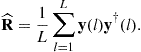 (21.215)
Under the hypothesis of a uniform true reflectivity and for a sufficient number of looks, ![]() may be used instead of
may be used instead of ![]() to perform tomography. The number of sources,
to perform tomography. The number of sources, ![]() , is in general unknown and needs to be estimated from the measured data. Some commonly used Model Order (MO) selection techniques based on statistical approaches, e.g., ITC, MDL, AIC [69–71], may be used to determine
, is in general unknown and needs to be estimated from the measured data. Some commonly used Model Order (MO) selection techniques based on statistical approaches, e.g., ITC, MDL, AIC [69–71], may be used to determine ![]() . Once
. Once ![]() is determined, the eigenstructure matrices can be estimated from the sample covariance matrix
is determined, the eigenstructure matrices can be estimated from the sample covariance matrix
![]() (21.216)
(21.216)
where ![]() and
and ![]() are respectively estimated signal and noise subspaces.
are respectively estimated signal and noise subspaces.
2.21.4.3.3.1 Single polarization tomography
Using MB-InSAR data sets acquired for a given polarization channel, Single Polarization (SP) tomography can be derived from the data covariance matrix ![]() using classical mono-dimensional estimators like Beamforming, Capon and MUSIC estimator as well as multi-dimensional methods like maximum likelihood estimators and weighted subspace fitting approaches.
using classical mono-dimensional estimators like Beamforming, Capon and MUSIC estimator as well as multi-dimensional methods like maximum likelihood estimators and weighted subspace fitting approaches.
Mono-dimensional estimators. These approaches determine ![]() , an estimate of the elevation of the scatterers under observation, as the coordinates of the
, an estimate of the elevation of the scatterers under observation, as the coordinates of the ![]() largest local maxima of an continuous objective function
largest local maxima of an continuous objective function ![]() :
:
![]() (21.217)
(21.217)
For the classical Beamformer and Capon spectral estimation techniques, the objective function is given by the continuous estimate of the reflectivity, ![]() , defined as
, defined as
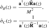 (21.218)
Once the set of scatterer elevation, ![]() , is estimated using (21.217), the corresponding reflectivities can be obtained from (21.218). The selection of discrete sources from peaks of the reflectivity spectrum confers to the Beamformer and Capon estimation techniques an important sensitivity to the acquisition configuration, and in particular to the presence of spurious sidelobes related to an irregular baseline sampling. The Beamformer is known to show a low resolution and may then overlook some closely spaced scatterers, whereas Capon’s technique possesses an improved resolution but a reduced radiometric accuracy.
, is estimated using (21.217), the corresponding reflectivities can be obtained from (21.218). The selection of discrete sources from peaks of the reflectivity spectrum confers to the Beamformer and Capon estimation techniques an important sensitivity to the acquisition configuration, and in particular to the presence of spurious sidelobes related to an irregular baseline sampling. The Beamformer is known to show a low resolution and may then overlook some closely spaced scatterers, whereas Capon’s technique possesses an improved resolution but a reduced radiometric accuracy.
MUSIC is a subspace based mono-dimensional technique, whose objective function is a measure of the orthogonality between a steering vector ![]() and the estimated noise subspace
and the estimated noise subspace ![]() and is given by:
and is given by:
![]() (21.219)
(21.219)
Once ![]() , is determined by inserting (21.219) in (21.217), a Least-Square (LS) estimate of the complex reflectivity vector
, is determined by inserting (21.219) in (21.217), a Least-Square (LS) estimate of the complex reflectivity vector ![]() can be obtained [60,61].
can be obtained [60,61].
Nonparametric approaches like Beamforming and Capon, are generally used to globally appreciate the structure of a volumetric medium and the main trends of the continuous reflectivity distribution in elevation. For the analysis of discrete spectral components, they may fail to discriminate closely spaced scatterers due either to their limited resolution, or to the presence of side lobes that may induce an erroneous estimation of the source location. MUSIC generally presents better performances for the analysis of discrete sources, related to a better resolution. Nevertheless, like all parametric methods, MUSIC is sensitive to data modeling errors, and in particular those related to the estimated number of sources ![]() . Moreover, MUSIC is known to work well in the case of uncorrelated scatterers, but its performance may degrade significantly in the presence of correlated scatterers since the source signal covariance matrix tends to be singular [72]. One of the main advantages of such techniques resides in the low numerical complexity of the mono-dimensional optimization described in (21.217).
. Moreover, MUSIC is known to work well in the case of uncorrelated scatterers, but its performance may degrade significantly in the presence of correlated scatterers since the source signal covariance matrix tends to be singular [72]. One of the main advantages of such techniques resides in the low numerical complexity of the mono-dimensional optimization described in (21.217).
Multi-dimensional estimators. Maximum likelihood (ML) estimators are multi-dimensional techniques, generally given by
![]() (21.220)
(21.220)
with the likelihood function ![]() . In the case of distributed scatterers, the Stochastic ML (SML) can be derived [73]:
. In the case of distributed scatterers, the Stochastic ML (SML) can be derived [73]:
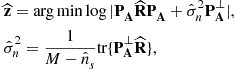 (21.221)
where ![]() represents the orthogonal projector on the null space of
represents the orthogonal projector on the null space of ![]() . Considering deterministic scatterers, the cost function (21.220) results in the Deterministic ML (DML) estimator[74]
. Considering deterministic scatterers, the cost function (21.220) results in the Deterministic ML (DML) estimator[74]
![]() (21.222)
(21.222)
Weighted Noise subspace fitting (NSF) estimator is derived by fitting the estimated noise subspace ![]() with
with ![]() in the weighted LS sense as follows:
in the weighted LS sense as follows:
![]() (21.223)
(21.223)
whereas the weighted Signal Subspace Fitting (SSF) cost function is given by:
![]() (21.224)
(21.224)
where the fitting matrix ![]() is replaced by its LS estimate
is replaced by its LS estimate ![]() . Both cost functions may be used to estimate the elevation of the scatters using a
. Both cost functions may be used to estimate the elevation of the scatters using a ![]() -dimensional minimization:
-dimensional minimization:
![]() (21.225)
(21.225)
where the suffix WSF indicates ones of the methods, NSF or SSF, mentioned above. It has been shown in [75], that any hermitian positive semi definite weighting matrix ![]() yields consistent parameter estimates. In particular, a consistent estimate of
yields consistent parameter estimates. In particular, a consistent estimate of ![]() permits to obtain minimum variance estimates, which asymptotically reach the Cramr-Rao lower bound [73]. Such a value is given for each case:
permits to obtain minimum variance estimates, which asymptotically reach the Cramr-Rao lower bound [73]. Such a value is given for each case:
 (21.226)
Compared with the mono-dimensional ones, multi-dimensional methods ML estimators are more robust, leading to global optima, but at an expensive computational cost. Regarding weighted subspace fitting techniques, the appropriate selection of certain weighting matrices can provide these estimators an optimal estimation accuracy as ML techniques at a reduced computational cost.
Numerical examples. In order to demonstrate the performance of the aforementioned tomographic estimators, two scatterers are assumed to locate at ![]() and
and ![]() , acquired respectively by a multibaseline configuration with
, acquired respectively by a multibaseline configuration with ![]() acquisitions. The baselines are assumed to be evenly distributed and between each successive acquisitions, the difference of vertical wavenumbers is supposed to be
acquisitions. The baselines are assumed to be evenly distributed and between each successive acquisitions, the difference of vertical wavenumbers is supposed to be ![]() . Assuming these two scatterers with equal reflectivity, the covariance matrix of source signals is given by
. Assuming these two scatterers with equal reflectivity, the covariance matrix of source signals is given by
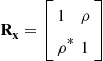
and ![]() . Varying the correlation factor
. Varying the correlation factor ![]() can respectively represent the source covariance matrix of coherent (
can respectively represent the source covariance matrix of coherent (![]() ), distributed (
), distributed (![]() ), and hybrid scatterers (
), and hybrid scatterers (![]() ). In order to study the vertical resolution, these estimators are used in the height estimation of uncorrelated signals (
). In order to study the vertical resolution, these estimators are used in the height estimation of uncorrelated signals (![]() ) with varying the height difference of two scatterers
) with varying the height difference of two scatterers ![]() . Figure 21.79a shows when
. Figure 21.79a shows when ![]() , MUSIC estimator degrades significantly due to closely spaced scatterers. SSF and NSF estimators both provide very good resolution with
, MUSIC estimator degrades significantly due to closely spaced scatterers. SSF and NSF estimators both provide very good resolution with ![]() . Whereas, Capon’s method can provide a good height estimate when
. Whereas, Capon’s method can provide a good height estimate when ![]() . Now simulating a 256-look sample data covariance matrix with varying
. Now simulating a 256-look sample data covariance matrix with varying ![]() from
from ![]() to
to ![]() , RMSE of the estimated
, RMSE of the estimated ![]() is plotted with respect to the correlation factor
is plotted with respect to the correlation factor ![]() in Figure 21.79b. The NSF estimator provides the most accurate estimate for uncorrelated or partially correlated signals (
in Figure 21.79b. The NSF estimator provides the most accurate estimate for uncorrelated or partially correlated signals (![]() ), while the SSF estimator copes well with highly correlated signals (
), while the SSF estimator copes well with highly correlated signals (![]() ). MUSIC cannot deal with highly correlated sources due to the quasi-singularity of
). MUSIC cannot deal with highly correlated sources due to the quasi-singularity of ![]() .
.

2.21.4.3.3.2 Fully polarimetric tomography
Fully Polarimetric (FP) tomography is implemented by jointly using fully polarimetric data sets acquired in a Polarimetric MB-InSAR configuration. It is a useful tool to extract both the scatterer’s vertical location and its scattering mechanism. Similar to the SP case, the FP tomography is derived from the data covariance matrix ![]() using some mono-dimensional and multi-dimensional FP spectral estimators.
using some mono-dimensional and multi-dimensional FP spectral estimators.
Mono-dimensional estimators. The elevation and scattering mechanisms of the different scatterers are estimated as the coordinates of the ![]() largest local maxima of a polarimetric objective function
largest local maxima of a polarimetric objective function ![]() .
.
![]() (21.227)
(21.227)
Similarly to the SP case, the Beamformer and Capon objective functions are given by continuous estimates of the reflectivity ![]() , with
, with
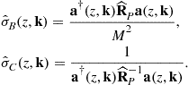 (21.228)
The direct local maximization of the FP objective function in (21.227) would require searching solutions in a 5-D argument space. Rewriting the polarimetric steering vector as
![]() (21.229)
(21.229)
permits to formulate reduce the search dimension to one, since
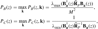 (21.230)
where ![]() represents the minimum and maximum eigenvalue of the positive semi-definite matrix
represents the minimum and maximum eigenvalue of the positive semi-definite matrix ![]() . Once the
. Once the ![]() elevations, are determined from the local maxima of (21.230), the corresponding scattering mechanisms can be estimated from:
elevations, are determined from the local maxima of (21.230), the corresponding scattering mechanisms can be estimated from:
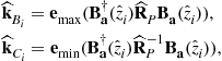 (21.231)
where ![]() indicates the eigenvector of
indicates the eigenvector of ![]() associated with
associated with ![]() , respectively. A similar approach may be applied to concentrate the FP MUSIC objective function:
, respectively. A similar approach may be applied to concentrate the FP MUSIC objective function:
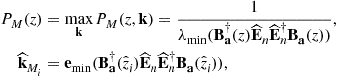 (21.232)
where ![]() represent here the eigenvectors of
represent here the eigenvectors of ![]() spanning its noise space. The reflectivity of the sources can be estimated, using a L-look polarimetric LS approach.
spanning its noise space. The reflectivity of the sources can be estimated, using a L-look polarimetric LS approach.
These estimators are considered as mono-dimensional, since the estimation of the elevation and the scattering mechanism is jointly realized by eigendecomposition. Such methods are computationally efficient but may reach some of the limitations mentioned in the SP case.
Multi-dimensional estimators. The ML estimators are formulated in the FP case using the polarimetric steering matrix ![]() , represented by:
, represented by:
To directly optimize the FP ML estimators, the estimation of ![]() optimal elevations
optimal elevations ![]() and target vectors
and target vectors ![]() , requires an optimization over a
, requires an optimization over a ![]() -dimensional space, and implies an excessive computational burden.
-dimensional space, and implies an excessive computational burden.
Polarimetric WSF estimators are given by:
Directly minimizing the FP-SSF estimator also suffers ![]() computational cost, but the FP-NSF estimator can maintain the computational cost as the SP case, using an analytic solution proposed in [66]. Compared with SP tomography, polarimetric tomography can provide more accurate localization of scatterers in the vertical direction due to the polarization diversity. The observed media can be further characterized in terms of both vertical location and scattering mechanism.
computational cost, but the FP-NSF estimator can maintain the computational cost as the SP case, using an analytic solution proposed in [66]. Compared with SP tomography, polarimetric tomography can provide more accurate localization of scatterers in the vertical direction due to the polarization diversity. The observed media can be further characterized in terms of both vertical location and scattering mechanism.
Numerical examples. Under the same baseline configuration as the SP case in Section (2.21.4.3.3.1), a 256-look sample covariance matrix is derived from received fully polarimetric data sets in the MB-PolInSAR configuration, which contains both height and polarimetric information. Assuming the above two scatterers with the canonical surface scattering, i.e., ![]() , Figure 21.80a shows RMSE of height estimation w.r.t.
, Figure 21.80a shows RMSE of height estimation w.r.t. ![]() : FP-Capon estimator still cannot accurately separate two scatterers due to a limited resolution; FP-NSF estimator provides the most precise height estimate; FP-MUSIC estimator degrades its performance for highly correlated scatterers. To study the role that polarization diversity plays in source separation, we denote Polarization Difference Angle
: FP-Capon estimator still cannot accurately separate two scatterers due to a limited resolution; FP-NSF estimator provides the most precise height estimate; FP-MUSIC estimator degrades its performance for highly correlated scatterers. To study the role that polarization diversity plays in source separation, we denote Polarization Difference Angle ![]() with
with ![]() . We keep the same surface scattering for the scatterer at 0 m and vary the scattering mechanism of the scatterer at 4 m to increase the polarization difference angle. As shown in Figure 21.80b, with
. We keep the same surface scattering for the scatterer at 0 m and vary the scattering mechanism of the scatterer at 4 m to increase the polarization difference angle. As shown in Figure 21.80b, with ![]() increasing, polarization diversity between two scatterers improves the height resolution, especially for FP-Capon estimator which reaches the same resolution as MUSIC when
increasing, polarization diversity between two scatterers improves the height resolution, especially for FP-Capon estimator which reaches the same resolution as MUSIC when ![]() . FP-NSF estimator performs best over all the polarization difference angle.
. FP-NSF estimator performs best over all the polarization difference angle.
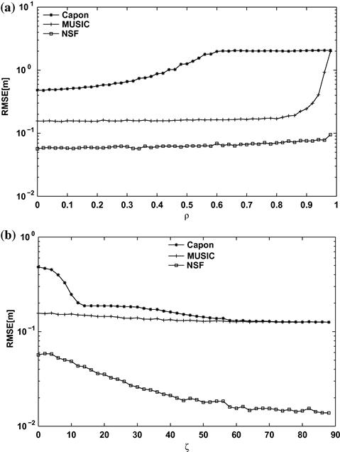
2.21.4.3.4 Applications
Using MB-PolInSAR data sets, TomSAR and PolTomSAR techniques are applied to retrieve the distribution of the backscattered power in the vertical direction, leading to 3-D images of observed scenes. These techniques permit to analyze volumic structures like forests, sand, snow, ice, etc. Some examples are given to illustrate the potentials of tomographic techniques in the applications of urban, forestry remote sensing and underfoliage imaging.
2.21.4.3.4.1 Urban remote sensing
High-resolution (HR) tomographic techniques are applied to analyze dense urban areas in terms of scatterers’ heights and their scattering mechanisms. Diverse scattering patterns can be encountered over dense urban environments, such as double bounce reflection at the wall-ground interaction, surface scattering from the roof and the ground, volumic scattering or a mixture of several scattering patterns. Conventional tomographic estimators may reach some limitations. The proposed model-adaptive FP-NSF estimator in [66,76] illustrates an undeniable performance using L-band intermediate-resolution dualbaseline FP data sets acquired over Dresden, Germany, by the DLR ESAR sensor. Over a test line, the ![]() tomograms obtained by FP-MUSIC and FP-NSF estimators with model order equal to 2 are shown in Figure 21.81. The heights of buildings are validated against LIDAR data as shown in [77]. FP-MUSIC estimator suffers spurious sidelobes (blue1 circle), whereas FP-NSF estimator illustrates precisely the vertical profile of buildings without any sidelobe. The 3-D reconstructions of an urban zone are depicted in Figure 21.82.
tomograms obtained by FP-MUSIC and FP-NSF estimators with model order equal to 2 are shown in Figure 21.81. The heights of buildings are validated against LIDAR data as shown in [77]. FP-MUSIC estimator suffers spurious sidelobes (blue1 circle), whereas FP-NSF estimator illustrates precisely the vertical profile of buildings without any sidelobe. The 3-D reconstructions of an urban zone are depicted in Figure 21.82.

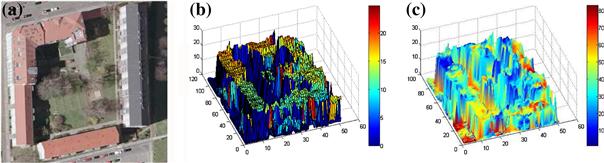
2.21.4.3.4.2 Forestry remote sensing
In the forest scenario, the canopy consists of a large number of elementary scatterers distributed in the vertical direction and is characterized by a continuous spectrum, whereas the ground is an impenetrable medium that possesses an isolated localized phase center and is characterized by a discrete spectrum. So the vertical distribution of backscattered power from forested areas leads to a mixed spectrum. The performance of conventional tomographic estimators may degrade due to their lack of adaptation to the type of spectrum. A novel hybrid tomographic approach is proposed to deal with the mixed spectrum and provides robust estimates for both tree top heights ![]() and the underlying ground topography
and the underlying ground topography ![]() [77].
[77].
Using P-band data sets (including 6 tracks) acquired over a test area of Paracou, French Guiana, by the ONERA SETHI sensor, the tree top and the ground elevation over an azimuth cut are estimated by the hybrid spectral approach (in gray) and the corresponding Lidar profiles (in black) are drawn over the normalized Capon tomograms in Figure 21.83. It can be observed that the estimated profiles coincide well with the Lidar ones. The ground elevation is precisely estimated using HH data sets, but still overestimated in VV and HV polarization. The forest top heights are well-estimated over all polarization channels. Using FP data sets, the results are similar to those obtained by HH data. Using HH data sets, Figure 21.84 depicts the estimated ![]() and
and ![]() over a test zone as well as the corresponding Lidar data in ground range. Globally, the estimated
over a test zone as well as the corresponding Lidar data in ground range. Globally, the estimated ![]() and
and ![]() match well with the Lidar ones in terms of texture and heights, except for some overestimated areas due to topographic effects that may influence scattering responses.
match well with the Lidar ones in terms of texture and heights, except for some overestimated areas due to topographic effects that may influence scattering responses.
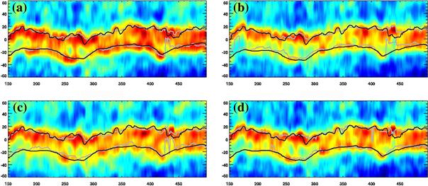
Figure 21.83 Tree top heights and underlying ground topography by TomSAR approaches. Black line: Lidar profiles. Gray line: estimated profiles by TomSAR. Vertical: height (m). Horizontal: azimuth (bin) (a) HH, (b) VV, (c) HV, and (d) FP (For interpretation of the references to color in this figure legend, the reader is referred to the web version of this book.).
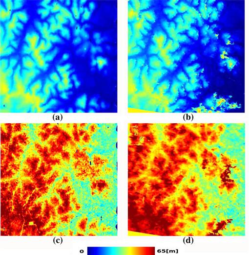
2.21.4.3.4.3 Underfoliage imaging
For the study of under-foliage imaging, Capon’s method has been applied to extract the shape of objects and canopy profile [78], but considering the complex structure of such objects, HR approaches are required to discriminate their closely spaced scattering features in the vertical direction. The performance of these spectral analysis techniques is conditioned by the statistical nature of the scattering response of the observed objects, as it has been shown in [79,80]. Under-foliage objects may be described by a deterministic response embedded within a speckle affected environment and hence associated to a series of complex scattering centers. To distinguish under-foliage objects, Figure 21.85 illustrates the ![]() tomograms over a test line with a truck beneath the canopy [81], using L-band PolInSAR data sets acquired over Dornstetten, Germany. The 3-D tomogram of the area, performed over azimuth bins and for varying range positions using the SP-SSF approach. Limiting the reconstruction height to 4 m above the terrain permits to isolate the under-foliage truck response (Figure 21.86a). Its reconstructed shape is similar to the uncovered one, with a reflectivity slightly higher (about 5 dB more) than the surrounding environment one. Complementary to distinct the objects in reflectivity, a 3-D reconstruction using FP-NSF estimator, permits to visualize the corresponding scattering pattern by
tomograms over a test line with a truck beneath the canopy [81], using L-band PolInSAR data sets acquired over Dornstetten, Germany. The 3-D tomogram of the area, performed over azimuth bins and for varying range positions using the SP-SSF approach. Limiting the reconstruction height to 4 m above the terrain permits to isolate the under-foliage truck response (Figure 21.86a). Its reconstructed shape is similar to the uncovered one, with a reflectivity slightly higher (about 5 dB more) than the surrounding environment one. Complementary to distinct the objects in reflectivity, a 3-D reconstruction using FP-NSF estimator, permits to visualize the corresponding scattering pattern by ![]() value. To better visualize the underlying truck response, the height is limited to 4 m above the ground and the reflectivity is limited to values inferior to 43 dB (Figure 21.86b). It shows that the truck outside the forest has a strong double bounce reflection at the ground-truck interaction, and the shape of the truck beneath the canopy is a precisely reconstructed with an
value. To better visualize the underlying truck response, the height is limited to 4 m above the ground and the reflectivity is limited to values inferior to 43 dB (Figure 21.86b). It shows that the truck outside the forest has a strong double bounce reflection at the ground-truck interaction, and the shape of the truck beneath the canopy is a precisely reconstructed with an ![]() value about
value about ![]() due to the sidelobe effect from the canopy. Using PolTomSAR techniques, the under-foliage truck can be well described both in terms of shape and scattering pattern.
due to the sidelobe effect from the canopy. Using PolTomSAR techniques, the under-foliage truck can be well described both in terms of shape and scattering pattern.
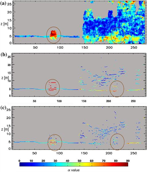
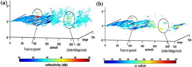
2.21.5 Conclusion and trends
As it has been mentioned in the introduction of this chapter, SAR polarimetry is a multi-disciplinary subject, with well-established theoretical foundations and tight connections with applied electromagnetism, multivariate signal processing, ![]()
Polarization diversity is particularly well adapted to SAR remote sensing since it provides both, a dimension over which one may filter out undesirable responses (or select responses of interest), and a very good way to characterize physical parameters of objects or media. Specific estimation techniques, adapted to the random nature of radar signals, have been developed to provide in an unsupervised way features that correspond to canonical scattering behaviors which can be efficiently used to determine a wide range of physical properties.
A comparison of a polarimetric color-coded SAR image with a single polarization one permits to realize that fully polarimetric measurements bring a lot more information and hence shall reveal much more useful. The most famous and widely used applications of SAR polarimetry mainly concern qualitative approaches, i.e., whose output parameter is not the estimate of the value of a physical parameter. Indeed, numerous polarization-based methods have been developed for object, or natural matter (like snow, water, ![]() ), or structure detection, environment classification and mapping in general, hazard monitoring, vegetation observation,
), or structure detection, environment classification and mapping in general, hazard monitoring, vegetation observation, ![]() For such applications, radar polarimetry provides very efficient tools that require among the smallest levels of supervision, i.e., that can be implemented in a quasi automatic way within badly known environments.
For such applications, radar polarimetry provides very efficient tools that require among the smallest levels of supervision, i.e., that can be implemented in a quasi automatic way within badly known environments.
Concerning quantitative approaches, the situation is slightly different. For some applications related to parameters that can be well separated by polarimetry, e.g., azimuthal orientation, or whose level of robustness may be estimated from the signal itself, radar polarimetry is a much valuable measuring approach. For some others, a reliable estimation may reveal difficult depending on the environment of the measure. For known conditions, a solution among the wide range offered by polarimetry can generally be found. In the opposite case, radar polarimetry may become a victim of the qualities of polarization. Polarization is widely used as diversity mode due to its good sensitivity to many of the electromagnetic properties of observed media. Estimating one particular parameter among the large number of other factors that modify the polarization of a wave and for a wide range of configurations can be problematic. Polarimetric measurements present a low dimensionality, 9 at most, while they do not possess any intrinsic structure, i.e., a target vector may be represented by an amplitude and a unitary vector. For applications, like those based on coherent spatial diversity, clutter echoes have low rank, whereas in the polarimetric case the clutter may occupy an important part of the eigen-space if the observed echos do not have sufficiently similar characteristics.
Current trends in SAR polarimetry correspond to different possible solutions considered to maintain polarimetry robustness to a high level even in particularly unfavorable configurations. Some solutions use external information provided by other types of sensors, like hyperspectral or other types of measurements.
Other particularly efficient solutions rely on incoherent diversity modes, based on the use of several spectral bands (carriers frequencies) or incidence angles or acquisition dates ![]() This solution is strongly encouraged by the development of space-borne sensors delivering time series of data sets.
This solution is strongly encouraged by the development of space-borne sensors delivering time series of data sets.
Finally coherent diversity modes, mainly based on spatial diversity using two (interferometry) or more (tomography) images have shown spectacular results. In particular, forest structure estimation using single or multi-baseline POL-inSAR acquisitions can give very good results when polarimetric only measurements are quasi-useless.
Anyway, one should avoid doing predictions about the future of radar polarimetry, since the historical review given in the introduction clearly mentions that radar polarimetry is regularly deeply modified by a surprising discovery!
This is why we really enjoy this research field.
References
1. Boerner WM. Inverse methods in electromagnetic imaging. In: Germany, Holland, Dordrecht: Reidel, Bad windsheim; 1983;Boerner Wolfgang M, ed. Nato Advanced Research Workshop on Inverse Methods in Electromagnetic Imaging. vol. 1–2.
2. G. Sinclair, Modification of the radar target equation for arbitrary targets and arbitrary polarization, Technical Report Report 302–19, The Ohio State University Research Foundation, Antenna Laboratory, 1948.
3. Sinclair S. The transmission and reception of elliptically polarized waves. Proc IRE. 1950;38(2):148–151.
4. E.M. Kennaugh, Effects of the type of polarization on echo characteristics, Technical Report 381–1 394–24, Antenna Laboratory, The Ohio State University Research Foundation, 1949.
5. Deschamps GA. Geometrical representation of the polarization of a plane electromagnetic wave. Proc IRE. 1951;39(5):540–544.
6. J. Huynen, Phenomenological theory of radar targets, PhD Thesis, Drukkerij Bronder-Offset NV, 1970.
7. Cloude SR. Group theory and polarisation algebra. OPTIK. 1986;75:26–36.
8. Freeman A. Sar calibration: an overview. IEEE Trans Geosci Remote Sens. 1992;30(6):1107–1121.
9. Freeman A, Durden S. A three-component scattering model for polarimetric sar data. IEEE Trans Geosci Remote Sens. 1998;36(3):963–973.
10. van Zyl J. Unsupervised classification of scattering behavior using radar polarimetry data. IEEE Trans Geosci Remote Sens. 1989;27(1):36–45.
11. Lee JS, Jurkevich L, Dewaele P, Wambacq P, Oosterlinck A. Speckle filtering of sar images: a review. Remote Sens Rev. 1994;8:313–340.
12. Cloude S, Pottier E. A review of target decomposition theorems in radar polarimetry. IEEE Trans Geosci Remote Sens. 1996;34(2):498–518.
13. Cloude S, Pottier E. An entropy based classification scheme for land applications of polarimetric sar. IEEE Trans Geosci Remote Sens. 1997;35(1):68–78.
14. Yamaguchi Y, Boerner W-M, Eom H, Sengoku M, Motooka S, Abe T. On characteristic polarization states in the cross-polarized radar channel. IEEE Trans Geosci Remote Sens. 1992;30(5):1078–1080.
15. Cloude S, Papathanassiou K. Polarimetric sar interferometry. IEEE Trans Geosci Remote Sens. 1998;36(5):1551–1565.
16. Lueneburg E. Direct and Inverse Electromagnetic Scattering. In: Harlow, UK: Addison Wesley Longman; 1996; Pittman Research Notes in Mathematic Series. vol. 361 Chapter Radar polarimetry: A revision of basc concepts.
17. Kostinski A, Boerner W. On foundations of radar polarimetry. IEEE Trans Antennas Propag. 1986;34(12):1395–1404.
18. Lee JS, Pottier E. Polarimetric Radar Imaging: From Basics to Applications. CRC Press 2008.
19. Lueneburg E. Principles of radar polarimetry. Proc IEICE Trans Electron Theory. 1995;10:1339–1345.
20. Cloude S. Lie groups in electromagnetic wave propagation and scattering. J Electromagnet Waves Appl. 1992;6(8):947–974.
21. Bamler R, Hartl P. Synthetic aperture radar interferometry. Inverse probl. 1998;14.
22. Lee J-S, Hoppel K, Mango S, Miller A. Intensity and phase statistics of multilook polarimetric and interferometric sar imagery. IEEE Trans Geosci Remote Sens. 1994;32(5):1017–1028.
23. Touzi R. A review of speckle filtering in the context of estimation theory. IEEE Trans Geosci Remote Sens. 2002;40(11):2392–2404.
24. S.R. Cloude, Polarimetry: the characterization of polarization effects in EM scattering, PhD Thesis, University of Birmingham, England, 1986.
25. Yamaguchi Y, Moriyama T, Ishido M, Yamada H. Four-component scattering model for polarimetric sar image decomposition. IEEE Trans Geosci Remote Sens. 2005;43(8):1699–1706.
26. Freeman A. Fitting a two-component scattering model to polarimetric sar data from forests. IEEE Trans Geosci Remote Sens. 2007;45(8):2583–2592.
27. Neumann M, Ferro-Famil L, Reigber A. Estimation of forest structure, ground, and canopy layer characteristics from multibaseline polarimetric interferometric sar data. IEEE Trans Geosci Remote Sens. 2009;48(3):1086–1104.
28. van Zyl J, Arii M, Kim Y. Model-based decomposition of polarimetric sar covariance matrices constrained for nonnegative eigenvalues. IEEE Trans Geosci Remote Sens. 2011;49(9):3452–3459.
29. Arii M, van Zyl J, Kim Y. Adaptive model-based decomposition of polarimetric sar covariance matrices. IEEE Trans Geosci Remote Sens. 2011;49(3):1104–1113.
30. Arii M, van Zyl J, Kim Y. A general characterization for polarimetric scattering from vegetation canopies. IEEE Trans Geosci Remote Sens. 2010;48(9):3349–3357.
31. Paladini R, Ferro-Famil L, Pottier E, Martorella M, Berizzi F, Dalle Mese E. Lossless and sufficient ![]() -invariant decomposition of random reciprocal target. IEEE Trans Geosci Remote Sens. 2012;99:1–15.
-invariant decomposition of random reciprocal target. IEEE Trans Geosci Remote Sens. 2012;99:1–15.
32. Ferro-Famil L, Pottier E, Lee JS. Unsupervised Classification of Natural Scenes form Polarimetric Interferometric SAR data. In: Frontiers of Remote Sensing Information Processing. World Scientific Publishing 2003;105–137.
33. Lee J-S, Jansen R, Schuler D, Ainsworth T, Marmorino G, Chubb S. Polarimetric analysis and modeling of multifrequency sar signatures from gulf stream fronts. IEEE J Oceanic Eng. 1998;23(4):322–333.
34. Lee J-S, Schuler D, Ainsworth T, Krogager E, Kasilingam D, Boerner W-M. On the estimation of radar polarization orientation shifts induced by terrain slopes. IEEE Trans Geosci Remote Sens. 2002;40(1):30–41.
35. Schuler D, Lee J-S, De Grandi G. Measurement of topography using polarimetric sar images. IEEE Trans Geosci Remote Sens. 1996;34(5):1266–1277.
36. Lee JS, Grunes MR, Pottier E, Ferro-Famil L. Unsupervised terrain classification preserving polarimetric scattering characteristics. IEEE Trans Geosci Remote Sens. 2004;42(4):722–731.
37. Hajnsek I, Pottier E, Cloude S. Inversion of surface parameters from polarimetric sar. IEEE Trans Geosci Remote Sens. 2003;41(4):727–744.
38. Fung A. Microwave Scattering and Emission Models and Their Applications. Artech House Remote Sensing Library, Artech House 1994; In: <http://books.google.fr/books?id=MHxtQgAACAAJ>; 1994.
39. Allain S, Ferro-Famil L, Pottier E. Relevant polarimetric parameters for surface parameter retrieval using multi-frequency sar data. In: Proceedings of the Fourth International Symposium on Retrieval of Bio- and Geophysical Parameters from SAR Data for Land Applications. 2004.
40. Allain S, Martinez CL, Ferro-Famil L, Pottier E. New eigenvalue-based parameters for natural media characterization. In: Proceedings of the IGARSS. 2005.
41. Chen K, Wu T-D, Tsang L, Li Q, Shi J, Fung A. Emission of rough surfaces calculated by the integral equation method with comparison to three-dimensional moment method simulations. IEEE Trans Geosci Remote Sens. 2003;41(1):90–101.
42. Leducq P, Ferro-Famil L, Pottier E. Matching-pursuit-based analysis of moving objects in polarimetric sar images. IEEE Geosci Remote Sens Lett. 2008;5(2):123–127.
43. Gatelli F, Guamieri A, Parizzi F, Pasquali P, Prati C, Rocca F. The wavenumber shift in sar interferometry. IEEE Trans Geosci Remote Sens. 1994;32(4):855–865.
44. Flandrin P. Time-Frequency/Time-Scale Analysis. London: Academic Press; 1999; (Wavelet Anlysis Appl.).
45. Ferro-Famil L, Boerner WM, Pottier E, Reigber A. Analysis of sar response anisotropic behavior using sub-aperture polarimetric data. In: Proceedings of the POLINSAR. 2003.
46. Ferro-Famil L, Reigber A, Pottier E, Boerner WM. Scene characterization using subaperture polarimetric sar data. IEEE Trans Geosci Remote Sens. 2003;41(10):2264–2276.
47. Yueh A, Shin RT, Kong JA. Scattering from randomly perturbed periodic and quasiperiodic surfaces. Prog Electromagnet Res. 1988;1:297–358.
48. Ferro-Famil L, Reigber A, Pottier E. Nonstationary natural media analysis from polarimetric sar data using a two-dimensional time-frequency decomposition approach. Can J Remote Sens. 2005;31(1):20–29.
49. Souyris J-C, Henry C, Adragna F. On the use of complex sar image spectral analysis for target detection: assessment of polarimetry. IEEE Trans Geosci Remote Sens. 2003;41(12):2725–2734.
50. Ferretti A, Prati C, Rocca F. Permanent scatterers in sar interferometry. IEEE Trans Geosci Remote Sens. 2001;39(1):8–20.
51. Schneider R, Papathanassiou K, Hajnsek I, Moreira A. Polarimetric and interferometric characterization of coherent scatterers in urban areas. IEEE Trans Geosci Remote Sens. 2006;44(4):971–984.
52. Spigai M, Tison C, Souyris J-C. Time-frequency analysis in high-resolution sar imagery. IEEE Trans Geosci Remote Sens. 2011;49(7):2699–2711.
53. Franceschetti G, Iodice A, Riccio D, Ruello G. Sar raw signal simulation for urban structures. IEEE Trans Geosci Remote Sens. 2003;41(9):1986–1995.
54. Ferro-Famil L, Pottier E. Urban area remote sensing from l- band polsar data using time-frequency techniques. In: Proceedings Urban Conference. 2007.
55. Cloude S. Polarization coherence tomography. Radio Sci. 2006;41(4):RS4017.
56. Cloude S, Papathanassiou K. Three-stage inversion process for polarimetric sar interferometry. IEE Proc Radar Sonar Navig. 2003;150(3):125–134.
57. Cloude SR. Polarisation Applications in Remote Sensing. Oxford University Press 2009.
58. Papathanassiou K, Cloude S. Single-baseline polarimetric sar interferometry. IEEE Trans Geosci Remote Sens. 2001;39(11):2352–2363.
59. Ferro-Famil L, Neumann M, Huang Y. Robust estimation of multi-baseline pol-insar parameters for the analysis of natural environments. In: Proceedings of the EUSAR. 2010.
60. Gini F, Lombardini F. Multibaseline cross-track sar interferometry: a signal processing perspective. IEEE Aerosp Electron Syst Mag. 2005;20(8):71–93.
61. Stoica P, Moses R. Spectral Analysis of Signals. Upper Saddle River, NJ: Prentice Hall; 2005.
62. Reigber A, Moreira A. First demonstration of airborne sar tomography using multibaseline l-band data. IEEE Trans Geosci Remote Sens. 2000;38(5):2142–2152.
63. Tebaldini S. Algebraic synthesis of forest scenarios from multibaseline polinsar data. IEEE Trans Geosci Remote Sens. 2009;47(12):4132–4142.
64. Tebaldini S. Single and multipolarimetric sar tomography of forested areas: a parametric approach. IEEE Trans Geosci Remote Sens. 2010;48(5):2375–2387.
65. Tebaldini S, Rocca F. Multibaseline polarimetric sar tomography of a boreal forest at p- and l-bands. IEEE Trans Geosci Remote Sens. 2012;50(1):232–246.
66. Huang Y, Ferro-Famil L, Reigber A. Under-foliage object imaging using sar tomography and polarimetric spectral estimators. IEEE Trans Geosci Remote Sens. 2011;99:1–13.
67. Gini F, Lombardini F, Montanari M. Layover solution in multibaseline sar interferometry. IEEE Trans Aerosp Electron Syst. 2002;38(4):1344–1356.
68. Sauer S, Ferro-Famil L, Pottier E, Reigber A. Physical parameter extraction over urban areas using l-band polsar data and interferometric baseline diversity. In: IEEE International Geoscience and Remote Sensing Symposium IGARSS 2007. 2007;1–5.
69. Wax M, Kailath T. Detection of signals by information theoretic criteria. IEEE Trans Acoust Speech Signal Process. 1985;33.
70. Wax M, Ziskind I. Detection of the number of coherent signals by the mdl principle. IEEE Trans Acoust Speech Signal Process. 1989;37(8):1190–1196.
71. Wax M, Ziskind I. Detection and localization of multiple sources via the stochastic signal model. IEEE Trans Signal Process. 1991;39(11):2450–2456.
72. Stoica P, Sharman K. Maximum likelihood methods for direction-of-arrival estimation. IEEE Trans Acoust Speech Signal Process. 1990;38(7):1132–1143.
73. Ottersten B, Viberg M, Stoica P, Nehorai A. Radar array processing. In: Exact and Large Sample Approximations of Maximum Likelihood Techniques for Parameter Estimation and Detection in Array Processing. Springer-Verlag 1993;99–151.
74. Stoica P, Ottersten B, Viberg M, Moses R. Maximum likelihood array processing for stochastic coherent sources. IEEE Trans Signal Process. 1996;44(1):96–105.
75. Viberg M, Ottersten B. Sensor array processing based on subspace fitting. IEEE Trans Signal Process. 1991;39(5):1110–1121.
76. Huang Y, Ferro-Famil L. 3d characterization of buildings in a dense urban environment using l-band pol-insar data with irregular baselines. In: Proceedings of the IGARSS. 2009.
77. Huang Y, Ferro-Famil L, Lardeux C. Polarimetric sar tomography of tropical forest at p-band. In: Proceedings of the IGARSS. 2011.
78. Nannini M, Scheiber R, Horn R. Imaging of targets beneath foliage with sar tomography. In: Proceedings of the EUSAR. 2008.
79. Huang Y, Ferro-Famil L. Building height estimation using multibaseline l-band sar data and polarimetric subspace fitting methods. In: Proceedings of the POLINSAR. 2009.
80. Stoica P, Nehorai A. Performance study of conditional and unconditional direction-of-arrival estimation. IEEE Trans Acoust Speech Signal Process. 1990;38(10):1783–1795.
81. Huang Y, Ferro-Famil L, Reigber A. Under foliage object imaging using sar tomography and polarimetric spectral estimators. In: Proceedings of the EUSAR. 2010.
1For interpretation of color in Figures 21.66, 21.82, 21.83 the reader is referred to the web version of this book.