Chapter 16
In-Phase and Quadrature (IQ) Signals

This chapter will explore amplitude modulation in a little more detail. The objectives are

1. To take a brief look at broadcast amplitude-modulated (AM) signals

2. To examine double-sideband suppressed carrier (DSBSC) AM signals

3. To use the DSBSC signal to generate I and Q signals

4. To determine how I and Q signals are demodulated

5. To apply I and Q signals to software-defined radios (SDRs)

Broadcast AM signals are generally modulated with a carrier signal and an audio signal. There is only one phase of carrier signal, and in the standard envelope detection of the AM radio signal, this phase information is normally not used. The standard AM signal is known as an amplitude-modulated signal with carrier. This signal is illustrated in Figure 16-1 and characterized by Equation (16-1).

FIGURE 16-1 An example waveform of a broadcast AM signal with 50 percent modulation.

All the waveforms have the X axis denoting time and the Y axis denoting amplitude.

This equation describes the waveform in Figure 16-1, with the modulation m of the carrier equal to 0.5, or 50 percent. If m = 100 percent, the carrier momentarily drops to zero or gets “pinched” off (Figure 16-2).

FIGURE 16-2 An AM signal with 100 percent modulation.

Figure 16-2 shows an AM signal that has been modulated at a 100 percent level, which pinches off the carrier but also allows the amplitude of the carrier to increase to twice its level at 0 percent modulation. In general, the equation governing the standard AM signal is

The modulating signal m(t) is limited in range generally in the following manner to prevent distortion when demodulating the AM signal:

Given this limitation in range for m(t), the value of [1 + m(t)] is nonnegative, and the phase of the carrier signal [cos(2πf_carrier) t] does not change as its carrier amplitude is being varied. The constant 1 in the term [1 + m(t)] ensures that there is a carrier signal should the modulating signal drop to 0. This makes sense because when the music or voice signals drop in a broadcast AM radio program, the radio-frequency (RF) carrier signal is still present.

Introduction to Suppressed-Carrier Amplitude Modulation

For a suppressed-carrier amplitude-modulated signal, there is no carrier signal. That is, the sinusoidal signal cos(2πf_carrier)t is not present in a suppressed-carrier AM signal. There are generally two types of suppressed-carrier AM signals, a double-sideband suppressed-carrier (DSBSC) AM signal and a signal-sideband suppressed-carrier (SSBSC) AM signal. By using a combination of DSBSC AM signals, one can also generate phase-modulated signals.

The basic signal to provide I and Q signals and single-sideband signals is the double-sideband signal S(t)_DSBSC. It is characterized by the following equation:

where V_sig(t) is the modulating signal and generally is an alternating-current (AC) signal, and the range of V_sig(t) is not necessarily restricted to –1 and +1. Figure 16-3 provides an illustration of a double-sideband suppressed-carrier signal S(t)_DSBSC. The figure looks rather strange in that one may expect to see that a sinusoidal modulating signal should result in a sinusoid envelope.

FIGURE 16-3 An example of a DSBSC (double-sideband suppressed-carrier) AM signal.

Figure 16-4 then overlays the modulating signal on top of the DSBSC AM signal for clarity. One should now note that the phase of the carrier signal cos(2πf_carrier)t can change signs or phase from 0 to 180 degrees and vice versa. For example, if for a particular duration V_sig(t) = + 1, then

FIGURE 16-4 The DSBSC AM signal with the modulating signal overlayed.

and the phase of the carrier is 0 degrees. However, for another duration V_sig(t) = –1, then

which means that the carrier signal has inverted or changed in phase by 180 degrees.

Figure 16-5 shows a relationship between the modulating signal, the DSBSC AM signal, and the carrier signal. The figure shows a continuous-wave (CW) carrier signal below the DSBSC AM signal. Note that in the regions where the modulating signal is positive (above 0), the positive peaks of the CW carrier signal line up with the positive peaks of the DSBSC AM signal. However, when the modulating signal is negative (below 0), we see that the positive peaks of the CW carrier signal line up with the negative peaks of the DSBSC AM signal. Thus a DSBSC AM signal includes time-varying amplitude and phase modifications on the carrier signal.

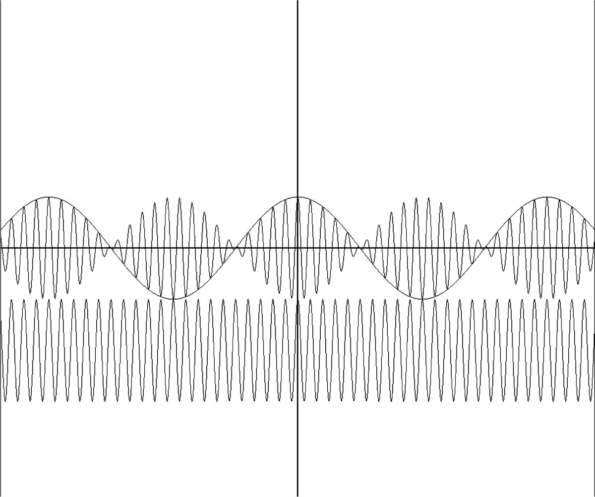
FIGURE 16-5 An illustration of the carrier signal as a reference phase compared with the DSBSC AM signal and modulating signal.

As mentioned previously, the DSBSC (double-sideband suppressed-carrier) AM signal with an AC modulating signal never contains the carrier signal. For example, if

then

As expected, multiplying the modulation signal (e.g., audio) by the carrier signal results in two signals whose frequencies are above and below the carrier frequency f_carrier by f_mod. The frequency (f_carrier + f_mod) is the upper-sideband frequency, and the (f_carrier–f_mod) frequency is the lower-sideband frequency.

In terms of demodulating the DSBSC (double sideband suppressed carrier) signal, simple envelope detection such as using a diode is not workable. A simple diode envelope detector will result in a demodulated signal that is distorted and full-wave rectified. For example, a sinusoidal modulating signal for the DSBSC signal will be detected with a diode, as shown in Figure 16-6.

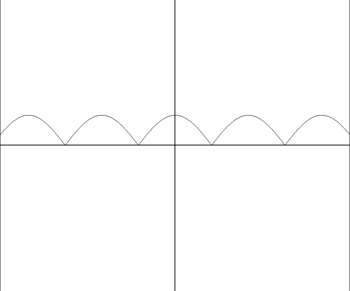
FIGURE 16-6 Using an envelope detector on a DSBSC AM signal results in full-wave rectification of the wanted signal.

From Figure 16-6 we see that simple envelope detection for the DSBSC AM signal results in distortion, and thus another way of detection is needed. Instead of a diode for demodulation, a synchronous detector is used.

A synchronous detector consists of a mixer or multiplier circuit and an oscillator that is precisely the same frequency as the carrier. The oscillator’s frequency sometimes can be adjusted to be near the original carrier frequency, but often a separate signal is sent to lock the oscillator to the correct frequency. An example of such a DSBSC AM system is the one used in recovering the L-R channels in a stereo FM radio. The L-R audio signals are DSBSC AM modulated by a 38-kHz oscillator at the radio station, and the spectrum of this AM signal spans from 23 to 53 kHz, with the carrier missing at 38 kHz. At the receiver, to regenerate the 38-kHz carrier signal for synchronous detection, a 19-kHz “pilot” signal is sent from the radio station. By frequency multiplication of the 19-kHz pilot tone, a 38-kHz signal is generated and then used to recover the L-R audio signals (Figure 16-7).

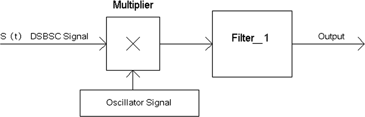
FIGURE 16-7 A demodulation system for a DSBSC AM signal.

The figure shows a demodulation system for a DSBSC AM signal by means of a mixer, oscillator, and low-pass filter. The received signal S(t)_DSBSC is connected to one of the inputs of the mixer or multiplier, whereas the remaining input of the mixer is connected to the oscillator that “somehow” has the correct frequency. After mixing the two signals, the mixer is connected to a low-pass filter to extract the modulation signal such as audio. Is this all that is needed to demodulate the signal S(t)_DSBSC? No, to demodulate the signal correctly, the phase of the oscillator’s signal is important.

Let’s take at look at Equation (16-3) to see why the phase of the receiver’s oscillator signal is important:

To demodulate this signal, we will multiply S(t)_DSBSC by a signal 2cos[(2πf_carriert + θ] that has the same carrier frequency and includes an arbitrary phase-shift angle θ. Then

The first term in this equation is a high-frequency signal of frequency 2πf_carrier that will be removed by the low-pass filter, leaving only the second term related to the cos(θ).

Thus the output via low-pass filtering is

If the phase angle θ from the receiver’s oscillator is 0, then the cos(θ) = cos(0) = 1, and we can see that the original modulating signal is recovered completely:

But if the oscillator’s phase is 90 degrees, the filtered output is

And if the oscillator’s phase is 180 degrees off from the radio station’s carrier signal phase, we get as the output

What’s interesting about using synchronous detection on a DSBSC AM signal is that with the “wrong” phase provided by the oscillator, the output of the detector can be zero. This result is almost as if the detector does not even “see” the input signal [V_sig(t)]cos(2πf_carrier)t.

At first look, this result of having the wrong phase from the oscillator for the detector may be a flaw in trying to demodulate a DSBSC (double-sideband suppressed-carrier) AM signal. But actually one can use this “flaw” to transmit two DSBSC AM signals (I and Q signals) and recover two channels of information, even though the two I and Q DSBSC AM signals occupy the same spectrum or bandwidth.

How I and Q Signals Are Generated

Before the structures of various I and Q modulators are shown, a table of trigonometric identities will be useful because generating various forms of I and Q signals involves multiplication of sine and cosine signals (Table 16-1).

Table 16-1 Trigonometric Identities

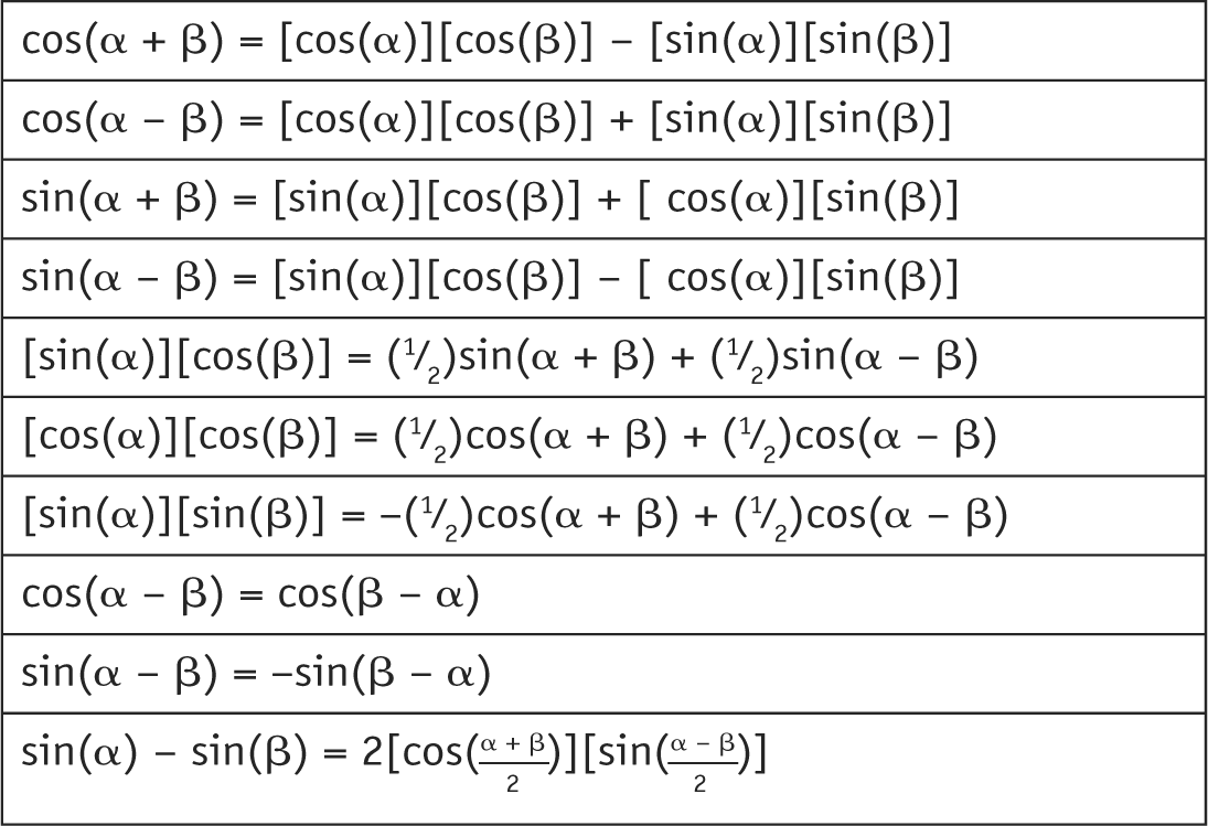
Figure 16-8 shows a general I and Q modulator. The figure shows a first input signal V₁(t) that is multiplied by an in-phase (I) carrier signal, generally a cosine signal such as cos(2πf_ct), where f_c is the carrier’s frequency in hertz. Similarly, the second input signal V₂(t) is multiplied by a quadrature-phase (Q) carrier signal that is 90 degrees phase-shifted from the I carrier signal, which is generally denoted as a sine signal such as sin(2πf_ct). Note that the carrier frequency f_c is the same for both I and Q carrier signals.

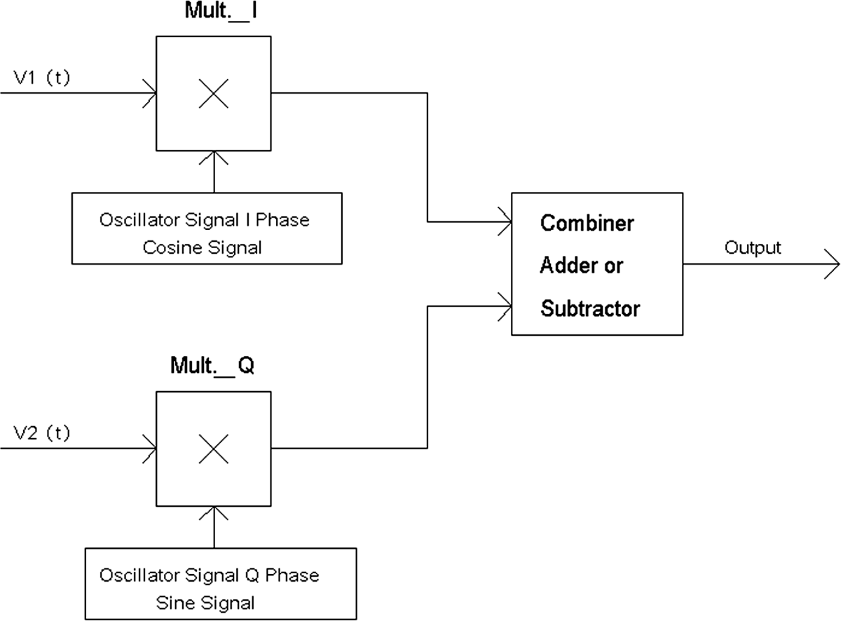
FIGURE 16-8 I and Q modulators using two mixers.

A combiner takes the output signals from each multiplier (M1 and M2) and can add or subtract them. The output of the combiner then provides a new signal.

I and Q signals that are combined have multiple uses. They are

1. Transmitting two separate channels of information within the same spectrum.

2. Frequency translating a signal of one frequency to another frequency, such as generating a single-sideband signal. The frequency shift can be upward or downward.

An example of transmitting two channels of information using I and Q signals or, equivalently, using quadrature modulation is the analog composite color television signals for NTSC (National Television System Committee) and PAL (Phase Alternate Line). Although television signals have been changed to a digital format, analog TV signals are still in use in many countries, even if the analog TV signals are not transmitted. DVD and Blu-ray disc players still have analog TV outputs, and many modern TV sets still have analog TV inputs. The use of quadrature modulation allows sending two channels of color video signals along with the luminance or black-and-white signal to provide decoding for red, green, and blue signals. When the outputs of the mixers are summed, the resulting signal is as follows:

To generate a single-sideband signal, we provide input signal V₂(t) as a 90-degree phase-shifted version of V₁(t). For simplicity, let V₁(t) = cos(2πf_modt) and V₂(t) = sin(2πf_modt), and now take the summed output signal as

By using two trigonometric identities from Table 16-1, namely,

and

let α = 2πf_modt and β = 2πf_ct and then

And by the trigonometric identity

If the combiner is a subtractor, then the new signal at the output of the combiner is

And by using the trigonometric identities (16-8) and (16-9), we get

Note that to provide “perfect” single-sideband signals, not only the amplitudes of the input signals have to be exact, but also the phases of the carrier and input signals both must keep an exact 90-degree difference. In practice, the input signals may not be exactly the same amplitude-wise, and the mixers may not have identical conversion gain. However, adjustments can be made to the mixer’s conversion gain and/or to the input’s amplitude to match the overall amplitude for maximum cancellation of the undesirable sideband.

Now let’s take a closer look at what happens if there is a deviation from a 90-degree signal of Δφ in the carrier signal. However, this time we will work with a slight change in the product terms (Figure 16-9).

FIGURE 16-9 An alternate single-sideband generator with a slight phase-angle error in the Q carrier signal.

Figure 16-9 shows a single-sideband modulation system that provides a sine-wave output with an error of Δφ in the Q carrier signal. Note that Δφ <<1, where Δφ is measured in radians. Thus

The upper-sideband terms are

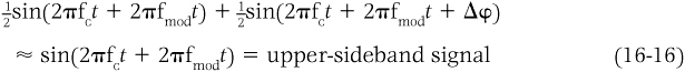
The lower-sideband signal would cancel out completely if Δφ = 0, but for small errors, we have

Both these sinusoidal waveforms represent “vectors” of the lower-sideband signal that have the same magnitude but nearly the same direction. In other words, both sinusoidal waveforms almost cancel out each other owing to the subtraction process.

For Equation (16-17), the trigonometric identity sin(α) – sin(β) = 2[cos(α 1 b)/2][sin(α – b)/2] will be useful in determining the magnitude (MAG) of the lower-sideband signal. Thus

or equivalently,

If the phase angle of sin(2πf_ct – 2πf_modt) is 0, then the residual magnitude of the lower-sideband signal is

For small angles of Δφ, sin(Δφ) = Δφ; thus

therefore,

Thus the residual lower-sideband signal has a magnitude of (½) Δφ, where Δφ is measured in radians. For example, if the Q phase error is 0.573 degree, or 0.01 radian, then the residual sideband will be (½)(0.01) = 0.005, or 0.5 percent, of the upper-sideband signal’s amplitude.

A graph of 100{(½)[sin(2πf_ct – 2πf_modt + 0) – sin(2πf_ct – 2πf_modt + Δφ )]} is shown in Figure 16-10 to confirm Equation (16-18). From the preceding calculations, the graph should show a cosine function with a peak amplitude of 100 × 0.005, or 0.5.

Figure 16-10 shows a sinusoidal waveform with a peak amplitude of 0.5, which is the result of multiplying (½)[sin(2πf_ct – 2πf_modt + 0) – sin(2πf_ct – 2πf_modt + 0.01)] by 100. The Y axis is full scale at 2.5 from the origin.

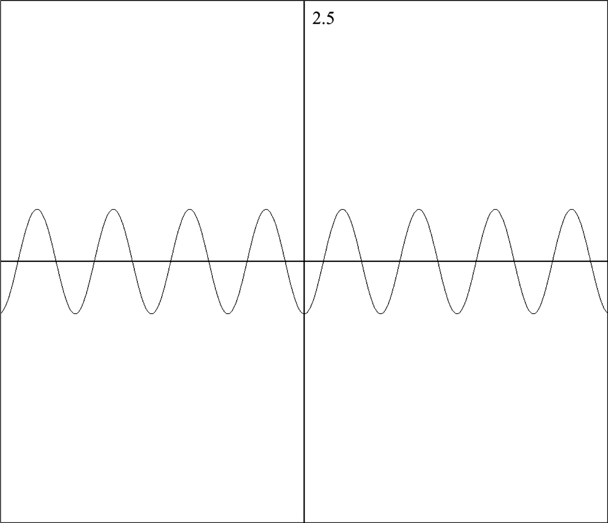
FIGURE 16-10 A graph of (1/2)[sin(2πf_ct – 2πf_modt + 0) – sin(2πf_ct – 2πf_modt + Δφ) multiplied 100-fold for ease of viewing.

The subtraction of two sine functions of almost the same phase leads to a cosine function. Intuitively, one would have thought two sine functions that close in phase would lead to another sine function. However, this “unexpected” result also provides another way to generate a Q signal. Of course, if one looks at the trigonometric tables, then one will see that this result is indeed expected. That is, two sine functions of nearly the same phase when subtracted do produce a cosine function.

In practice, the mixers can be of switch-mode type that generates square waves, which may be difficult to subtract with a differential amplifier. So an equivalent function can be made by inverting an input signal to an input of a mixer instead and then combine by adding via resistors. If switch-mode mixers are used, then a low-pass or band-pass filter should be used to remove harmonics from the combining circuit.

Demodulating I and Q Signals

When a summed I and Q signal is sent to a demodulator, there are two channels of information coexisting with each other without interfering with the delivery of information from each channel. In standard AM broadcast signals, to send a 5-kHz audio channel with standard AM signals that contain upper- and lower-sideband signals plus the carrier signal, 10 kHz of bandwidth in the RF channel is needed. However, if I and Q signals are sent instead with each 5 kHz of information, each I and Q channel occupies 10 kHz within the same channel space. Thus, when demodulated, two channels of 5 kHz of information are delivered, which is twice the information received for the same RF bandwidth when compared with standard broadcast AM signals. Because the I and Q signals are orthogonal to each other, the two signals are almost in different but parallel universes.

When both I and Q signals are combined, they may look “messy,” and at first glance, the I and Q signals seem inseparable. It is as if someone took a sheet of white paper and wrote an essay with blue ink from top to bottom and then wrote on the same page from top to bottom another essay in red ink. With the different essays written over each other, at first glance, one would find it difficult to read. But if a red filter is placed over the sheet, the writing in blue ink can be read, and likewise, if a blue filter is placed over the sheet, the writing in red ink can be read.

Demodulating I and Q signals is similar to the preceding description, and separating out each channel is done with multiplication of the I and Q signals with 0- and 90-degree signals.

Once the quadrature modulated signals are combined as described in Equation (16-6), a single wire or channel can be used to carry or transmit these signals to a receiver. To demodulate the two channels of information V₁(t) and V₂(t), an oscillator or signal source must have the same carrier frequency f_c during the modulation process. Normally, the signal source regenerates the frequency f_c. For example, in color TV signals, a phase-lock loop oscillator or regeneration oscillator along with a reference signal sent provides a demodulation signal with a frequency f_c at 0 and 90 degrees of phase.

Figure 16-11 shows a demodulation system consisting of two mixers and filters and two carrier signal sources. The output of the first mixer M1 then is

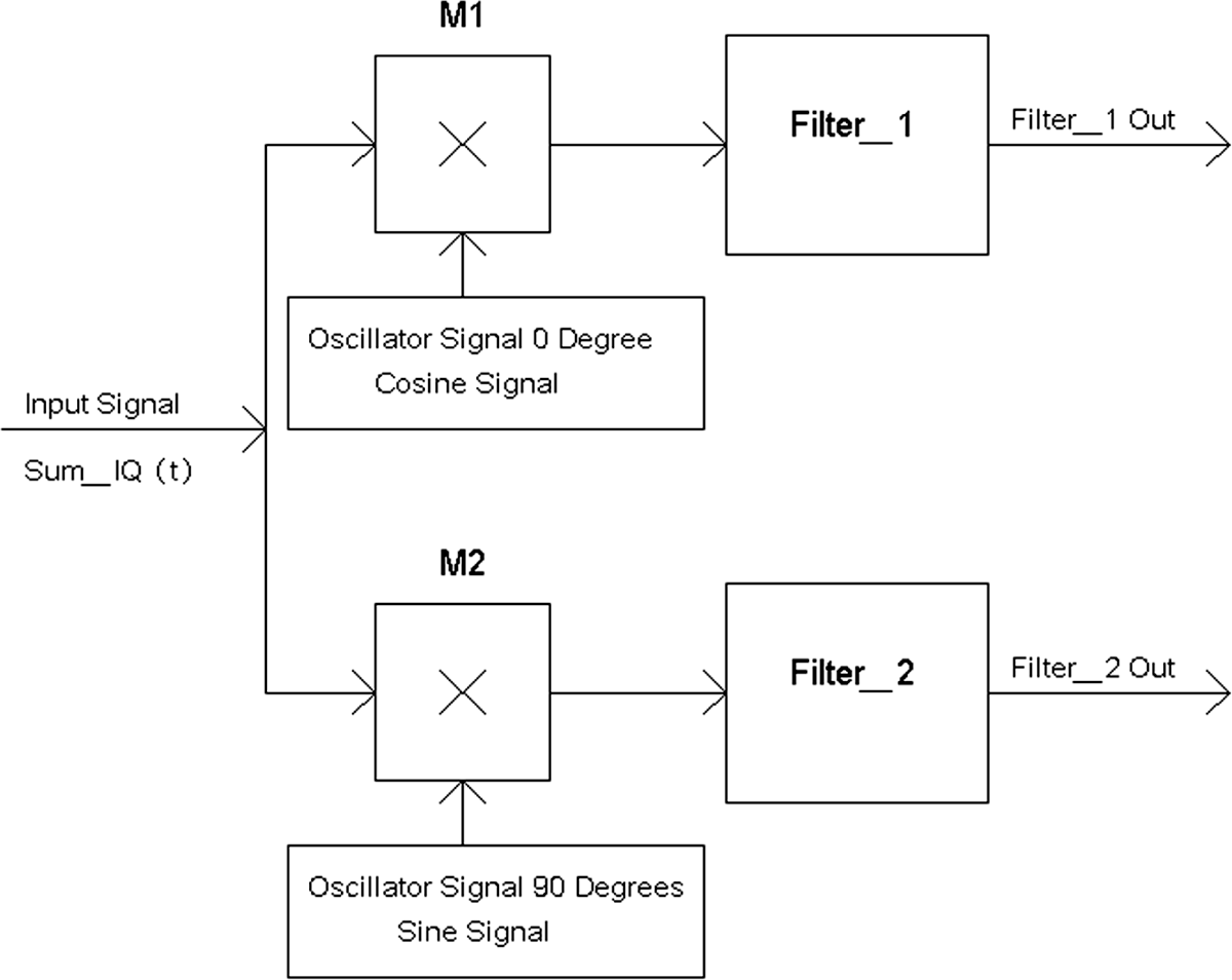
FIGURE 16-11 An IQ signal demodulation system.

To recover or demodulate V₁(t) while “ignoring” V₂(t), we multiply Sum_IQ(t) by a signal source = cos(2πf_ct). Therefore,

The high-frequency terms relating to 2π2f_ct are filtered out via low-pass or bandpass filtering and with cos(0) = 1 and sin(0) = 0. Also, whenever a sine wave and a cosine wave of the same frequency and phase are multiplied, the result is 0 after filtering out the high-frequency signals. The output of Filter_1 that is connected to M1 is then

Similarly to recover V₂(t), we multiply Sum_IQ(t) by signal sin(2πf_ct). Then

When the high-frequency terms from M2_out are filtered out, the output of Filter_2 results in

The demodulation of single-sideband signals, however, does not require an exact phase of the oscillator but does require an exact frequency. Most single-sideband signals are beyond the audio band of 10 kHz or 20 kHz. Thus the demodulation of these types of single-sideband signals is relatively easy by simple multiplication with the oscillator signal, whose frequency is the same as the oscillator frequency at the transmitting end.

For example, for demodulating an upper sideband signal

we need to multiply this signal, [Subtr_{IQ_usb}(t)], with cos(2πf_ct) and filter out the high-frequency signal. Thus we have

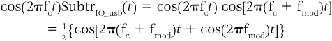
When the high-frequency signal cos[2π(f_c + f_mod)t] is filtered out, the result is

I and Q Signals Used in Software-Defined Radios (SDRs)

Another use for quadrature modulation is to transform a signal into two signals that are equal in amplitude and also have a relationship 0 and 90 degrees between each other. This transformation also changes the frequency from the original. For example, if a signal is at 10 MHz, quadrature modulation can provide two signals at 20 kHz that are 90 degrees apart from each other. Figure 16-12 shows a 0- and 90-degree phase shifter based on IQ or quadrature modulation.

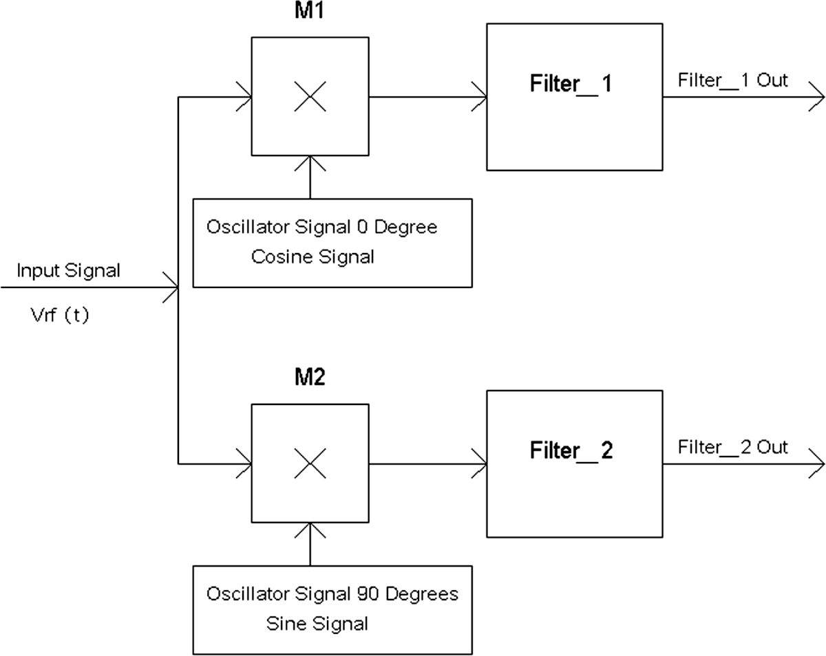
FIGURE 16-12 A 0- and 90-degree phasing circuit.

The figure shows a single signal source V_RF(t) = cos(2πf_RFt) that is connected to the input of two mixers M1 and M2. A signal generator cos(2πf_OSCt) is connected to the remaining input terminal of mixer M1, and another signal generator sin(2πf_OSCt) is connected to the remaining input of mixer M2.

The outputs of M1 and M2 are connected to filters Filter_1 and Filter_2, respectively. These filters remove the high-frequency signals from the outputs of the mixers. Therefore, the output of mixer M1 is

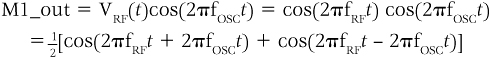
Filter_1 removes the higher-frequency signal, which results in

For mixer M2, the output is

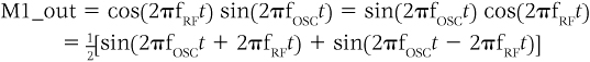
Filter_2 removes the higher-frequency signal, which results in

Therefore, the signals from Filter1_out and Filter2_out are 90 degrees apart from each other no matter how low a frequency (f_OSC – f_RF) is, even down to near direct currect (DC). Now the fact that these two signals can maintain a 90-degree difference all the way down to nearly DC is truly amazing. The I and Q signals from the filters then allow a computer to digitize these signals and demodulate them.

References

1. U.S. Patent 1,855,576, Clyde R. Keith, “Frequency Translating System,” filed on April 9, 1929.

2. U.S. Patent 2,086,601, Robert S. Caruthers, “Modulating System,” filed on May 3, 1934.

3. U.S. Patent 2,025,158, Frank Augustus Cowan, “Modulating System,” filed on June 7, 1934.

4. U.S. Patent 5,058,159, Ronald Quan, “Method and System for Scrambling and Descrambling Audio Information Signals,” filed on June 15, 1989.

5. U.S. Patent 5,159,531, Ronald Quan and Ali R. Hakimi, “Audio Scrambling System Using In-Band Carrier,” filed on April 26, 1990.

6. U.S. Patent 5,471,531, Ronald Quan, “Method and Apparatus for Low Cost Audio Scrambling and Descrambling,” filed on December 14, 1993.

7. U.S. Patent 6,091,822, “Method and Apparatus for Recording Scrambled Video Audio Signals and Playing Back Said Video Signal, Descrambled, Within a Secure Environment,” Andrew B. Mellows, John O. Ryan, William J. Wrobleski, Ronald Quan, and Gerow, D. Brill, filed on January 8, 1998.

8. Kenneth K. Clarke and Donald T. Hess, Communication Circuits: Analysis and Design. Reading: Addison-Wesley, 1971.

9. Thomas H. Lee, The Design of CMOS Radio-Frequency Integrated Circuits, 2nd ed. Cambridge: Cambridge University Press, 2003.

10. Donald O. Pederson and Kartikeya Mayaram, Analog Integrated Circuits for Communication. Boston: Kluwer Academic Publishers, 1991.

11. Allan R. Hambley, Electrical Engineering Principles and Applications, 2nd ed. Upper Saddle River: Prentice Hall, 2002.

12. Robert L. Shrader, Electronic Communication, 6th ed. New York: Glencoe McGraw-Hill, 1991.

13. Mischa Schwartz, Information, Transmission, and Noise. New York: McGraw-Hill, 1959.

14. Harold S. Black, Modulation Theory. Princeton: D. Van Nostrand Company, 1953.

15. B. P. Lathi, Linear Systems and Signals. Carmichael: Berkeley Cambridge Press, 2002.

16. Alan V. Oppenheim and Alan S. Wilsky, with S. Hamid Nawab, Signals and Systems, 2nd ed. Upper Saddle River: Prentice Hall, 1997.

17. Howard W. Coleman, Color Television. New York: Hastings House, Publishers, 1968.

18. Geoffrey Hutson, Peter Shepherd, and James Brice, Colour Television System Principles. 2nd ed. London: McGraw-Hill, 1990.

19. Mary P. Dolciani, Simon L. Bergman, and William Wooton, Modern Algebra and Trigonometry. New York: Houghton Mifflin, 1963.