Windowing

Abstract

This chapter throws light on the windowing, aiming to optimize finite impulse response (FIR) filter frequency response with a finite number of coefficients. The chapter explains the process of truncating of infinite number of coefficients through windowing that generate a desirable response. This is further elaborated through tapering of coefficients, which holds importance for designers to manage passband and stopband ripple with a trade-off of increasing the transition band. Lastly, with some relevant examples of coefficient windows, aspect of Windowing is supported in all FIR-related filter design software programs.

Keywords

Band-pass filter; Blackman window; Finite impulse response; Low-pass filter; Stopband; Windowing

In the previous chapter, we developed a technique for calculating filter coefficients to generate a desired frequency response. Our desired filter response will generate an infinite number of coefficients, and we have to decide how many coefficients to keep and throw away or truncate the rest. As the previous plots show, when the number of coefficients grows larger, the transition region from passband to stopband grows smaller, and the stopband rejection or attenuation increases.

$Frequency response = H (ω) = \sum_{i = - \infty to \infty} C_{i} e^{- j ω i}$ $Frequency response = H (ω) = \sum_{i = - \infty to \infty} C_{i} e^{- j ω i}$

The smaller transition region, or steepness of the transition from pass to stopband, is due to higher frequency components in the frequency response. The higher indexes of “i” in the frequency response correspond to higher frequency complex exponentials. Complex exponentials have a sinusoidal characteristic, so to get a quick response, one must use higher frequency exponentials.

6.1. Truncation of Coefficients

The process of truncating the infinite number of coefficients is called windowing. We can imagine C_{i= −∞ to ∞}, and multiplying it term by term with a window function, W_{i= −∞ to ∞}. Let us consider the examples of the plots in the previous chapter, with our low-pass filter with a cutoff frequency of π/2.

$C_{i} = (1 / π i) \cdot \sin (π i / 2) for - \infty < i < \infty$ $C_{i} = (1 / π i) \cdot \sin (π i / 2) for - \infty < i < \infty$

For our 7-tap filter,

$W_{i} = 1 for - 3 \leq i \leq 3 {and W}_{i} = 0 otherwise .$ $W_{i} = 1 for - 3 \leq i \leq 3 {and W}_{i} = 0 otherwise .$

Similarly, for our 15-tap filter

$W_{i} = 1 for - 7 \leq i \leq 7 {and W}_{i} = 0 otherwise .$ $W_{i} = 1 for - 7 \leq i \leq 7 {and W}_{i} = 0 otherwise .$

In both cases, W_i is a rectangular window. This means that the coefficients are unaltered within the window and are zeroed or truncated outside the window. The length of the rectangular window determined the length of the impulse response of the filter. This is called rectangular window because the window coefficients W_i are all “1” within the window and “0” outside.

With the rectangular window, we are abruptly truncating the impulse response of the filter. Obviously, for realistic filter implementations, we have to limit the impulse response at some point, as each tap or coefficient requires a multiply operation to compute each filter output. But perhaps we can get a more desirable response by reducing the coefficient values gradually at either end of the impulse response before we reach the point of impulse response truncation.

6.2. Tapering of Coefficients

This has led to efforts to develop other window functions besides the default rectangular window. Window design and analysis involved a fair bit of mathematics. But after the rigors of the last chapter, many readers will probably not mind too much if we skip over this. Actually, many filter designers do not know the details of the various window functions offered by their filter design software but work iteratively instead. That is, the designer will experiment with moving the frequency cutoff point slightly and playing the allowable number of taps, the various window options, and sometimes the numerical precision (number of bits) of the input data and coefficients. By observing the computer-generated frequency plots, the designer can iterate to find an optimum combination of these parameters that meet the application requirements.

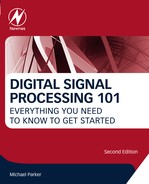
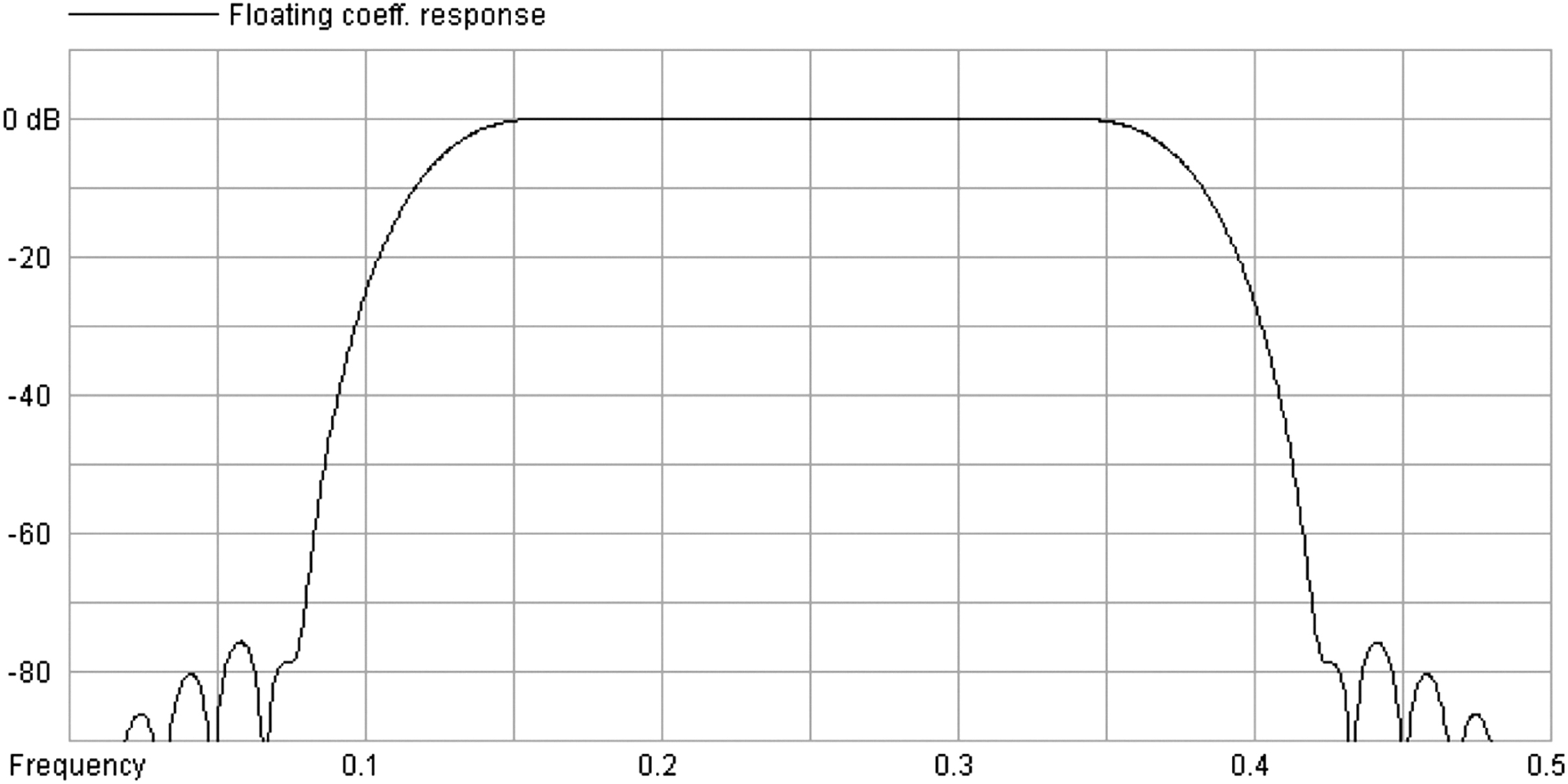
Often, the requirements will be a certain degree of filter rejection or attenuation at one or more specific frequency points, a maximum amount of ripple or variance in the passband region of the frequency response, and a specified region of the frequency response (Fig. 6.1).

Figure 6.1 Low-pass filter frequency response.

Most windows are named after their inventors. These include Hamming, von Hann, Kaiser, Blackman, Bartlett, and others. The window coefficients will not be equal to 1 as in the rectangular window but will gradually change from 1 to 0 in some fashion near the edges of the window. The form of this transition or tapering off of the coefficients defines the window properties. Note that this is a different function than filter design, which produced the original and ideal set of coefficients. Windowing is used to avoid the abrupt truncation of the filter coefficient set, required to allow implementation of the filter with a finite number of multiply–add operations.

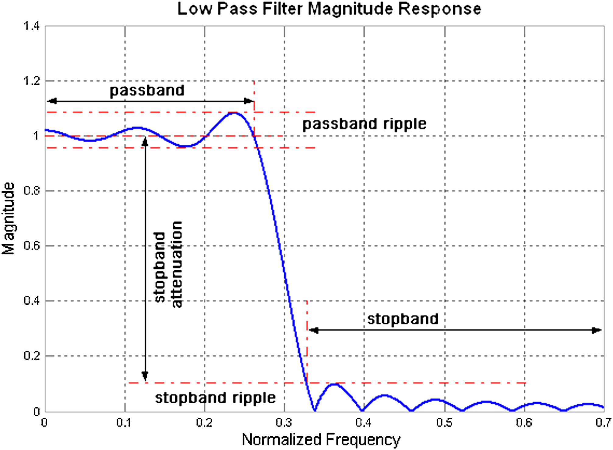
In general, a window cannot increase the steepness of the transition region, but it can be used to reduce either the passband or stopband ripple in the frequency response. Most filter design programs offer several window options. Below are the frequency responses with different windows for comparison. All the filters shown are for a 61-tap band-pass filter. The major trade-off between the different windows is the width of the transition band and the amount of attenuation in the stopband region of the frequency response. Often, the filter designer will make trade-offs in transition width, passband ripple, stopband attenuation (including rippler of lobes in stopband), number of coefficients, and the chosen window to achieve the application requirements.

6.3. Sample Coefficient Windows

Below in Figs. 6.2–6.5, several windows are shown with the rectangular window as the baseline. Notice that the rectangular window (Fig. 6.2) provides the steepest transition band. However, the stopband sidelobes are very high, reducing the amount of stopband attenuation. The Hanning, Hamming, and Blackman windows provide increasing stopband attenuation, at the expense of a wider transition band. Windowing is supported in all finite impulse response filter design software programs.

Figure 6.2 61-tap band-pass filter with rectangular window.

Figure 6.3 61-tap band-pass filter with Hanning window.

Figure 6.4 61-tap band-pass filter with Hamming window.

Figure 6.5 61-tap band-pass filter with Blackman window.

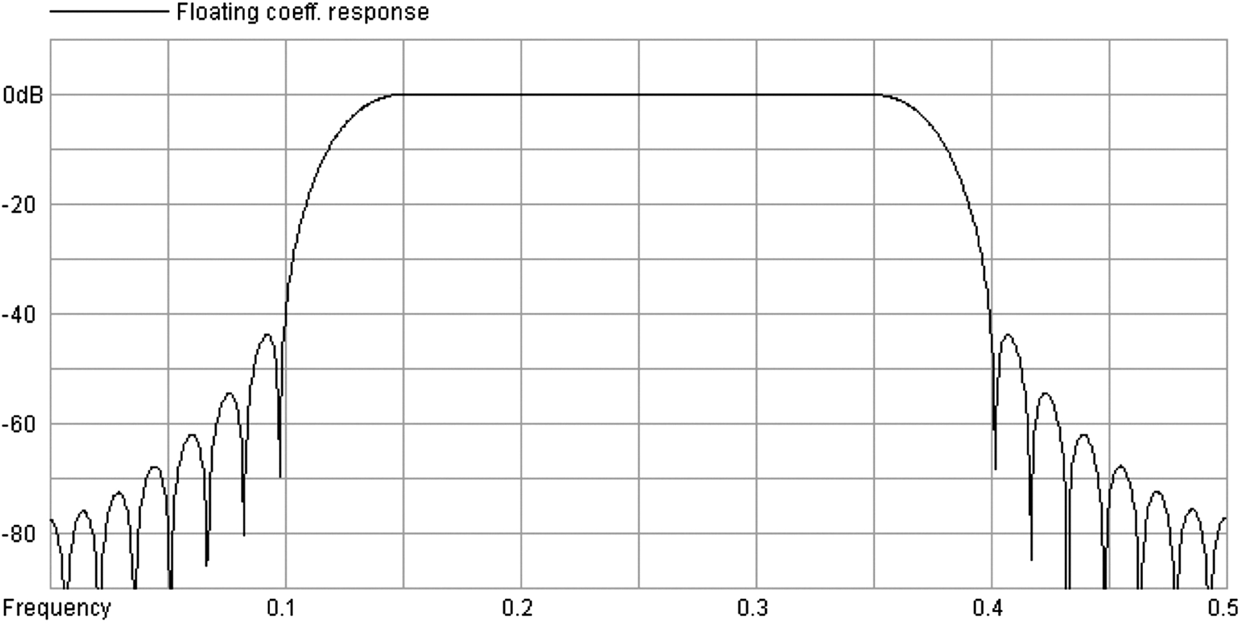
These windows have a similar effect on the transition band and sidelobes whether applied to low-pass filters, high-pass filters, or band-pass filters.

..................Content has been hidden....................

You can't read the all page of ebook, please click here login for view all page.

Table of Contents for Chapter 6. Windowing

Create new playlist

Sign In

Sign Up

Abstract

Keywords

6.1. Truncation of Coefficients

6.2. Tapering of Coefficients

6.3. Sample Coefficient Windows

Table of Contents for
Chapter 6. Windowing