Search in book...
Toggle Font Controls
Create new playlist

Name your new playlist

Playlist description (optional)
Sign In

Email address

Password

Forgot Password?

or

Continue with Facebook

Continue with Google
Sign Up

Full Name

Email address

Confirm Email Address

Password

or

Continue with Facebook

Continue with Google

Chapter 5

Finite Impulse Response (FIR) Filters

Abstract

This chapter explores the fundamentals of the finite infinite response filter, the workhorse of digital signal processing. It starts with the structure of finite impulse response (FIR) filter, the methods to build it, and the properties. The chapter shows how the number and value of the filter coefficients determine the frequency response of an filter. The characteristic of FIR filters is discussed in detail with emphasis so as to why it is preferred over other type of digital filters.

Keywords

Coefficients; Exponentials; Finite impulse response; Frequency; Nonzero input

This chapter will focus on the workhorse of digital signal processing (DSP)—the finite impulse response (FIR) filter. We are going to discuss three main topics. First we will talk about the structure of an FIR filter, how to build one, and some of its properties. Next we are going to show how, given the filter coefficients, to compute the frequency response of the filter (normally, this is done with software, but we can gain insight by understanding how to do this). Last, we will show a method to compute coefficients to meet a given frequency response. This last step is what is commonly required of a DSP designer—to find the number and value of filter coefficients required for frequency response required by the application. Again, this is normally done with software, but we need to gain insight as to what is involved. Filter design is a process where we cannot have everything, and compromise is necessary. To use software tools to design filters, we will need to understand what the different trade-offs are, and how they interact.

5.1. Finite Impulse Response Filter Construction

Let us begin with how to construct an FIR filter. An FIR filter is built of multipliers and adders. It can be implemented in hardware or software, and run in a serial fashion, parallel fashion, or some combination. We will focus on the parallel implementation, because it is the most straightforward to understand.

FIR filters, and DSP in general, often use delay elements. A delay element is simply a clocked register, and a series of delay elements is simply a shift register. However, in DSP, a one-sample delay element is often represented as a box with a z⁻¹ symbol. This comes from the mathematical properties of the z-transform, which we have not covered here in the interests of minimizing mathematics (although there is a discussion of z-transform in Appendix D). But we cannot skip the use of z⁻¹ representing a single clock or register delay, as it is prevalent in DSP diagrams and literature. We will use this here, so that you can get used to seeing this representation.

A key property of an FIR filter is the number of taps or multipliers required to compute each output. In a parallel implementation, the number of taps equals the number of multipliers. In a serial implementation, one multiplier is used to perform all of the multipliers sequentially for each output. Assuming single clock cycle multipliers, a parallel FIR filter can produce one output each clock cycle, and a serial FIR filter would require N clock cycles to produce each output, where N is the number of filter taps. Filters can sometimes have hundreds of taps. Below shown is a small 5-tap parallel filter (Fig. 5.1).

Figure 5.1 Finite impulse response filter structure.

The inputs and outputs of the FIR filter are sampled data. For simplicity, we will assume that the inputs, outputs, and filter coefficients C_m are all real numbers. The input data stream will be denoted as x_k and the output y_k. The “k” subscript is used to identify the sequence of data. For example, x_k+1 follows x_k, and x_k−1 precedes x_k. Often for the purpose of defining a steady state response, we assume that the data streams are infinitely long in time, or that k extends from –∞ to +∞.

The coefficients are usually static (meaning they do not change over time), and determine the filter's frequency response.

In equation form, the filter could be represented as:

$y_{k} = C_{0} \cdot x_{k} + C_{1} \cdot x_{k - 1} + C_{2} \cdot x_{k - 2} + C_{3} \cdot x_{k - 3} + C_{4} \cdot x_{k - 4}$ $y_{k} = C_{0} \cdot x_{k} + C_{1} \cdot x_{k - 1} + C_{2} \cdot x_{k - 2} + C_{3} \cdot x_{k - 3} + C_{4} \cdot x_{k - 4}$

It is just the sum of multipliers. This could get pretty tedious to write as the number of taps gets larger, so the following short hand summation is often used:

$y_{k} = \sum_{i = 0 to 4} C_{i} x_{k - i}$ $y_{k} = \sum_{i = 0 to 4} C_{i} x_{k - i}$

We can also make the equation for any length of filter. To make our filter of length “N,” we simply replace the 4 (5−1 taps) with N−1.

$y_{k} = \sum_{i = 0 to N - 1} C_{i} x_{k - i}$ $y_{k} = \sum_{i = 0 to N - 1} C_{i} x_{k - i}$

Another way to look at this is that the data stream …x_k+2, x_k+1, x_k, x_k−1, x_k−2… is sliding past a fixed array of coefficients. At each clock cycle, the data and coefficients are cross-multiplied and the outputs of all multipliers for that clock cycle are summed, to form a single output (this process also known as dot product). Then on the next clock cycle, the data is shifted one place relative to the coefficients (which are fixed), and the process repeated. This process is known as convolution.

The FIR structure is very simple, yet it has the ability to create almost any frequency response, given sufficient number of taps. This is very powerful, but unfortunately not at all intuitive. It's somewhat analogous to the brain—a very simple structure of interconnected neurons, yet the combination can produce amazing results. During the rest of the chapter, we will try to gain some understanding of how this happens.

Below is an example using actual numbers, to illustrate this process called convolution.

We will define a filter of 5 coefficients {C₀,C₁,C₂,C₃,C₄} = {1,3,5,3,1}.

Our x_k sequence will be defined as {x₀,x₁,x₂,x₃,x₄,x₅} = {−1,1,2,1,4,−1} and

x_k = 0 for k < 0 and for k > 6 (everywhere else).

Let us start by computing

y_{- 1} = \sum_{i = 0 to N - 1} C_{i} x_{- 1 - i}

$y_{- 1} = \sum_{i = 0 to N - 1} C_{i} x_{- 1 - i}$

We can see that the subscript on x will be negative for all i = 0 to 4. In this example y_k = 0 for k < 0. What this is saying, is that until there is a nonzero input x_k, the output y_k will also be zero. Things start to happen at k = 0, because x₀ is the first nonzero input.

$y_{- 1} = \sum_{i = 0 to N - 1} C_{i} x_{- 1 - i} = (1) (0) + (3) (0) + (5) (0) + (3) (0) + (1) (0) = 0$ $y_{- 1} = \sum_{i = 0 to N - 1} C_{i} x_{- 1 - i} = (1) (0) + (3) (0) + (5) (0) + (3) (0) + (1) (0) = 0$

$y_{0} = \sum_{i = 0 to N - 1} C_{i} x_{0 - i} = (1) (- 1) + (3) (0) + (5) (0) + (3) (0) + (1) (0) = - 1$ $y_{0} = \sum_{i = 0 to N - 1} C_{i} x_{0 - i} = (1) (- 1) + (3) (0) + (5) (0) + (3) (0) + (1) (0) = - 1$

$y_{1} = \sum_{i = 0 to N - 1} C_{i} x_{1 - i} = (1) (1) + (3) (- 1) + (5) (0) + (3) (0) + (1) (0) = - 2$ $y_{1} = \sum_{i = 0 to N - 1} C_{i} x_{1 - i} = (1) (1) + (3) (- 1) + (5) (0) + (3) (0) + (1) (0) = - 2$

$y_{2} = \sum_{i = 0 to N - 1} C_{i} x_{2 - i} = (1) (2) + (3) (1) + (5) (- 1) + (3) (0) + (1) (0) = 0$ $y_{2} = \sum_{i = 0 to N - 1} C_{i} x_{2 - i} = (1) (2) + (3) (1) + (5) (- 1) + (3) (0) + (1) (0) = 0$

$y_{3} = \sum_{i = 0 to N - 1} C_{i} x_{3 - i} = (1) (1) + (3) (2) + (5) (1) + (3) (- 1) + (1) (0) = 9$ $y_{3} = \sum_{i = 0 to N - 1} C_{i} x_{3 - i} = (1) (1) + (3) (2) + (5) (1) + (3) (- 1) + (1) (0) = 9$

$y_{4} = \sum_{i = 0 to N - 1} C_{i} x_{4 - i} = (1) (4) + (3) (1) + (5) (2) + (3) (1) + (1) (- 1) = 19$ $y_{4} = \sum_{i = 0 to N - 1} C_{i} x_{4 - i} = (1) (4) + (3) (1) + (5) (2) + (3) (1) + (1) (- 1) = 19$

$y_{5} = \sum_{i = 0 to N - 1} C_{i} x_{5 - i} = (1) (- 1) + (3) (4) + (5) (1) + (3) (2) + (1) (1) = 23$ $y_{5} = \sum_{i = 0 to N - 1} C_{i} x_{5 - i} = (1) (- 1) + (3) (4) + (5) (1) + (3) (2) + (1) (1) = 23$

$y_{6} = \sum_{i = 0 to N - 1} C_{i} x_{6 - i} = (1) (0) + (3) (- 1) + (5) (4) + (3) (1) + (1) (2) = 22$ $y_{6} = \sum_{i = 0 to N - 1} C_{i} x_{6 - i} = (1) (0) + (3) (- 1) + (5) (4) + (3) (1) + (1) (2) = 22$

$y_{7} = \sum_{i = 0 to N - 1} C_{i} x_{7 - i} = (1) (0) + (3) (0) + (5) (- 1) + (3) (4) + (1) (1) = 8$ $y_{7} = \sum_{i = 0 to N - 1} C_{i} x_{7 - i} = (1) (0) + (3) (0) + (5) (- 1) + (3) (4) + (1) (1) = 8$

$y_{8} = \sum_{i = 0 to N - 1} C_{i} x_{8 - i} = (1) (0) + (3) (0) + (5) (0) + (3) (- 1) + (1) (4) = 1$ $y_{8} = \sum_{i = 0 to N - 1} C_{i} x_{8 - i} = (1) (0) + (3) (0) + (5) (0) + (3) (- 1) + (1) (4) = 1$

$y_{9} = \sum_{i = 0 to N - 1} C_{i} x_{9 - i} = (1) (0) + (3) (0) + (5) (0) + (3) (0) + (1) (- 1) = - 1$ $y_{9} = \sum_{i = 0 to N - 1} C_{i} x_{9 - i} = (1) (0) + (3) (0) + (5) (0) + (3) (0) + (1) (- 1) = - 1$

$y_{10} = \sum_{i = 0 to N - 1} C_{i} x_{10 - i} = (1) (0) + (3) (0) + (5) (0) + (3) (0) + (1) (0) = 0$ $y_{10} = \sum_{i = 0 to N - 1} C_{i} x_{10 - i} = (1) (0) + (3) (0) + (5) (0) + (3) (0) + (1) (0) = 0$

$y_{11} = \sum_{i = 0 to N - 1} C_{i} x_{11 - i} = (1) (0) + (3) (0) + (5) (0) + (3) (0) + (1) (0) = 0$ $y_{11} = \sum_{i = 0 to N - 1} C_{i} x_{11 - i} = (1) (0) + (3) (0) + (5) (0) + (3) (0) + (1) (0) = 0$

$y_{12} = \sum_{i = 0 to N - 1} C_{i} x_{12 - i} = (1) (0) + (3) (0) + (5) (0) + (3) (0) + (1) (0) = 0$ $y_{12} = \sum_{i = 0 to N - 1} C_{i} x_{12 - i} = (1) (0) + (3) (0) + (5) (0) + (3) (0) + (1) (0) = 0$

This is definitely tedious. There are a couple of things to notice. Follow the input x₄ = 4 (highlighted) in our example. See how it moves across, from one multiplier to the next. Each input sample x_k will be multiplied by each tap in turn. Once it passes through the filter, that input sample is discarded and has no further influence on the output. In our example, x₄ is discarded after computing y₈.

Once the last nonzero input data x_k has shifted it's way through the filter taps, the output data y_k will go to zero (this starts at k = 10 in our example).

Now let us consider a special case, where x_k = 1 for k = 0, and x_k = 0 for k ≠ 0. This means that we only have one nonzero input sample, and it is equal to 1. Now if we again compute the output, which is simpler this time, we get:

$y_{0} = \sum_{i = 0 to N - 1} C_{i} x_{0 - i} = (1) (1) + (3) (0) + (5) (0) + (3) (0) + (1) (0) = 1$ $y_{0} = \sum_{i = 0 to N - 1} C_{i} x_{0 - i} = (1) (1) + (3) (0) + (5) (0) + (3) (0) + (1) (0) = 1$

$y_{1} = \sum_{i = 0 to N - 1} C_{i} x_{1 - i} = (1) (0) + (3) (1) + (5) (0) + (3) (0) + (1) (0) = 3$ $y_{1} = \sum_{i = 0 to N - 1} C_{i} x_{1 - i} = (1) (0) + (3) (1) + (5) (0) + (3) (0) + (1) (0) = 3$

$y_{2} = \sum_{i = 0 to N - 1} C_{i} x_{2 - i} = (1) (0) + (3) (0) + (5) (1) + (3) (0) + (1) (0) = 5$ $y_{2} = \sum_{i = 0 to N - 1} C_{i} x_{2 - i} = (1) (0) + (3) (0) + (5) (1) + (3) (0) + (1) (0) = 5$

$y_{3} = \sum_{i = 0 to N - 1} C_{i} x_{3 - i} = (1) (0) + (3) (0) + (5) (0) + (3) (1) + (1) (0) = 3$ $y_{3} = \sum_{i = 0 to N - 1} C_{i} x_{3 - i} = (1) (0) + (3) (0) + (5) (0) + (3) (1) + (1) (0) = 3$

$y_{4} = \sum_{i = 0 to N - 1} C_{i} x_{4 - i} = (1) (0) + (3) (0) + (5) (0) + (3) (0) + (1) (1) = 1$ $y_{4} = \sum_{i = 0 to N - 1} C_{i} x_{4 - i} = (1) (0) + (3) (0) + (5) (0) + (3) (0) + (1) (1) = 1$

$y_{5} = \sum_{i = 0 to N - 1} C_{i} x_{5 - i} = (1) (0) + (3) (0) + (5) (0) + (3) (0) + (1) (0) = 0$ $y_{5} = \sum_{i = 0 to N - 1} C_{i} x_{5 - i} = (1) (0) + (3) (0) + (5) (0) + (3) (0) + (1) (0) = 0$

$y_{6} = \sum_{i = 0 to N - 1} C_{i} x_{6 - i} = (1) (0) + (3) (0) + (5) (0) + (3) (0) + (1) (0) = 0$ $y_{6} = \sum_{i = 0 to N - 1} C_{i} x_{6 - i} = (1) (0) + (3) (0) + (5) (0) + (3) (0) + (1) (0) = 0$

Notice that output is the same sequence as the coefficients. This should come as no surprise once you think about it. This output is defined as the filter's impulse response, named as it occurs when the filter input is an impulse, or a single nonzero input equal to 1. This gives the FIR filter its name. By “finite impulse response” or FIR, this indicates that if this type of filter is driven with an impulse, we will see a response (the output) has a finite length, after which it becomes zero. This may seem trivial, but it is a very good property to have, as we will see in the chapter on infinite impulse response filters.

5.2. Computing Frequency Response

What we have covered so far is the mechanics of building the filter, and how to compute the output data, given the coefficients and input data. But we do not have any intuitive feeling as to how this operation can allow some frequencies to pass through, and block other frequencies. A very basic understanding of a low-pass filter can be gained by the concept of averaging. We all know that if we average multiply results, we get a smoother, more consistent output, and rapid fluctuations are damped out. A moving average filter is simply a filter with all the coefficients set to 1. The more filter taps, the longer the averaging, and the more smoothing takes place. This gives an idea of how a filter structure can remove high frequencies or rapid fluctuations. Now imagine if the filter taps were alternating +1, −1, +1 −1… and so on. A slowly varying input signal will have adjacent samples nearly the same, and these will cancel in the filter, resulting in a nearly zero output. This filter is blocking low frequencies. On the other hand, an input signal near the Nyquist rate will have big changes from sample to sample and will result in a much larger output. However, to get a more precise handle on how to configure the coefficient values to get the desired frequency response, we are going to need using a bit of math.

We will start by computing the frequency response of the filter from the coefficients. Remember, the frequency response of the filter is determined by the coefficients (also called the impulse response).

Let us begin by trying to determine the frequency response of a filter by measurement. Imagine if we take a complex exponential signal of a given frequency and use this as the input to our filter. Then we measure the output. If the frequency of the exponential signal is in the passband of the filter, it will appear at the output. But if the frequency of the exponential signal is in the stopband of the filter, it will appear at the output with a much lower level than the input, or not at all. Imagine we start with a very low frequency exponential input, and do this measurement, then slightly increase the frequency of the exponential input, measure again, and keep going until the exponential frequency is equal to the Nyquist frequency. If we plot the level of the output signal across the frequency from 0 to F_Nyquist, we will have the frequency response of the filter. It turns out that we do not have to do all these measurements, instead we can compute this fairly easily. This is shown below.

$y_{k} = \sum_{i = 0 to 4} C_{i} x_{k - i}$ $y_{k} = \sum_{i = 0 to 4} C_{i} x_{k - i}$	Output of our 5-tap example filter
$y_{k} = \sum_{i = - \infty to \infty} C_{i} x_{k - i}$ $y_{k} = \sum_{i = - \infty to \infty} C_{i} x_{k - i}$	Same equation, except that we are allowing infinite number of coefficients (no limits on filter length)
x_m = e^jωm = cos(ωm) + j sin(ωm)	This is our complex exponential input at ω radians per sample.

Let us take a close look at the last equation, and review a bit.

It is just a sampled version of a signal rotating around the unit circle. We sample at time = m, and then sample again at time = m + 1. So from one sample to the next, our sampled signal will move ω radians around the unit circle. If we are sampling at 10 times faster than we are moving around the unit circle, then it will take 10 samples to get around the circle and move 2π/10 radians each sample.

$x_{m} = e^{j 2 π m / 10} = \cos (2 π m / 10) + j \sin (2 π m / 10) when ω = 2 π / 10$ $x_{m} = e^{j 2 π m / 10} = \cos (2 π m / 10) + j \sin (2 π m / 10) when ω = 2 π / 10$

To clarify, an example table below shows x_m = e^j2πm/10 evaluated at various m. If you want to check using a calculator, remember that the angles are in units of radians, not degrees (Table 5.1).

We could also increment x_m so that we rotate the unit circle every five samples. This is twice as fast as before. Hopefully you are getting more comfortable with complex exponentials.

$x_{m} = e^{j 2 π m / 5} = \cos (2 π / 5) + j \sin (2 π m / 5) when π = 2 π / 5$ $x_{m} = e^{j 2 π m / 5} = \cos (2 π / 5) + j \sin (2 π m / 5) when π = 2 π / 5$

Table 5.1

Evaluating Complex Exponentials

m = 0	x₀ = e^j0 = cos (0) + j sin (0)	1 + j0
m = 1	x₁ = e^jπ/5 = cos (π/5) + j sin (π/5)	0.8090 + j0.5878
m = 2	x₂ = e^j2π/5 = cos (2π/5) + j sin (2π/5)	0.3090 + j0.9511
m = 3	x₃ = e^j3π/5 = cos (3π/5) + j sin (3π/5)	−0.3090 + j0.9511
m = 4	x₄ = e^j4π/5 = cos (4π/5) + j sin (4π/5)	−0.8090 + j0.5878
m = 5	x₅ = e^jπ = cos (π) + j sin (π)	−1 + j0
m = 6	x₆ = e^j6π/5 = cos (6π/5) + j sin (6π/5)	−0.8090 −j0.5878
m = 7	x₇ = e^j7π/5 = cos (7π/5) + j sin (7π/5)	−0.3090 −j0.9511
m = 8	x₈ = e^j8π/5 = cos (8π/5) + j sin (8π/5)	0.3090 − j0.9511
m = 9	x₉ = e^j9π/5 = cos (9π/5) + j sin (9π/5)	0.8090 − j0.5878
m = 10	x₁₀ = x₀ = e^j2π = cos (2π) + j sin (2π)	1 + j0

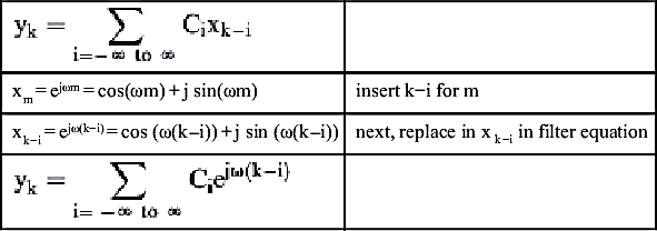
Now we go back to the filter equation and substitute the complex exponential input for x_k-i.

$y_{k} = \sum_{i = - \infty to \infty} C_{i} x_{k - i}$ $y_{k} = \sum_{i = - \infty to \infty} C_{i} x_{k - i}$
x_m = e^jωm = cos(ωm) + j sin(ωm)	insert k−i for m
x_k−i = e^jω(k−i) = cos (ω(k−i)) + j sin (ω(k−i))	next, replace in x_k−i in filter equation
$y_{k} = \sum_{i = - \infty to \infty} C_{i} e^{j ω (k - i)}$ $y_{k} = \sum_{i = - \infty to \infty} C_{i} e^{j ω (k - i)}$

There is a property of exponentials that we frequently need to use.

$e^{(a + b)} = e^{a} \cdot e^{b} and e^{(a - b)} = e^{a} \cdot e^{- b}$ $e^{(a + b)} = e^{a} \cdot e^{b} and e^{(a - b)} = e^{a} \cdot e^{- b}$

If you remember your scientific notation, this makes sense. For example,

$10^{2} \cdot 10^{3} = 100 \cdot 1000 = 100,000 = 10^{5} = 10^{(2 + 3)}$ $10^{2} \cdot 10^{3} = 100 \cdot 1000 = 100,000 = 10^{5} = 10^{(2 + 3)}$

OK, now back to the filter equation.

$y_{k} = \sum_{i = - \infty to \infty} C_{i} e^{j ω (k - i)} = \sum_{i = - \infty to \infty} C_{i} e^{j ω k} \cdot e^{- j ω i}$ $y_{k} = \sum_{i = - \infty to \infty} C_{i} e^{j ω (k - i)} = \sum_{i = - \infty to \infty} C_{i} e^{j ω k} \cdot e^{- j ω i}$

Let us do a little algebra trick. Notice that the term e^jωk does not contain the term i used in the summation. So we can pull this term out in front of the summation.

$y_{k} = e^{j ω k} \cdot \sum_{i = - \infty to \infty} C_{i} e^{- j ω i}$ $y_{k} = e^{j ω k} \cdot \sum_{i = - \infty to \infty} C_{i} e^{- j ω i}$

Notice that the term e^jωk is just the complex exponential we used as an input.

$y_{k} = x_{k} \cdot \sum_{i = - \infty to \infty} C_{i} e^{- j ω i}$ $y_{k} = x_{k} \cdot \sum_{i = - \infty to \infty} C_{i} e^{- j ω i}$

Voila! The expression

\sum_{i = - \infty to \infty} C_{i} e^{- j ω i}

$\sum_{i = - \infty to \infty} C_{i} e^{- j ω i}$

gives us the value of the frequency response ofthe filter at frequency ω. It is solely a function of ω and the filter coefficients.

This expression applies a gain factor to the input, x_k, to produce the filter output. Where this expression is large, we are in the passband of the filter. If this expression is close to zero, we are in stopband of the filter.

Let us give this expression a less cumbersome representation. Again, it is a function of ω, which we expect, because the characteristics of the filter vary with frequency. It is also a function of the coefficients, C_i, but these are assumed fixed for a given filter.

$Frequency response = H (ω) = \sum_{i = - \infty to \infty} C_{i} e^{- j ω i}$ $Frequency response = H (ω) = \sum_{i = - \infty to \infty} C_{i} e^{- j ω i}$

Now in reality, it is not as bad as it looks. This is the generic version of the equation, where we must allow for an infinite number of coefficients (or taps). But suppose we are determining the frequency response of our 5-tap example filter.

$H (ω) = \sum_{i = 0 to 4} C_{i} e^{- j ω i} and {C 0, C 1, C 2, C 3, C 4} = {1,3,5,3,1}$ $H (ω) = \sum_{i = 0 to 4} C_{i} e^{- j ω i} and {C 0, C 1, C 2, C 3, C 4} = {1,3,5,3,1}$

Let us find the response of the filter at a couple different frequencies. First, let ω = 0. This corresponds to DC input—we are putting a constant level signal into the filter. This would be x_k = 1 for all values k.

$H (0) = C_{0} + C_{1} + C_{2} + C_{3} + C_{4} = 1 + 3 + 5 + 3 + 1 = 13$ $H (0) = C_{0} + C_{1} + C_{2} + C_{3} + C_{4} = 1 + 3 + 5 + 3 + 1 = 13$

This one was simple, since e⁰ = 1. The DC or zero frequency response of the filter is called the gain of the filter. Often, it may be convenient to force the gain = 1, which would involve dividing all the individual filter coefficients by H(0). The passbands and stopbands characteristics are not altered by this process, since all the coefficients are scaled equally. It just normalizes the frequency response so the passband has a gain equal to 1.

Now compute the frequency response for ω = π/2.

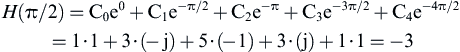
$\begin{matrix} H (π / 2) = C_{0} e^{0} + C_{1} e^{- π / 2} + C_{2} e^{- π} + C_{3} e^{- 3 π / 2} + C_{4} e^{- 4 π / 2} \\ = 1 \cdot 1 + 3 \cdot (- j) + 5 \cdot (- 1) + 3 \cdot (j) + 1 \cdot 1 = - 3 \end{matrix}$ $\begin{matrix} H (π / 2) = C_{0} e^{0} + C_{1} e^{- π / 2} + C_{2} e^{- π} + C_{3} e^{- 3 π / 2} + C_{4} e^{- 4 π / 2} \\ = 1 \cdot 1 + 3 \cdot (- j) + 5 \cdot (- 1) + 3 \cdot (j) + 1 \cdot 1 = - 3 \end{matrix}$

So the magnitude of the frequency response has gone from 13 (at ω = 0) to 3 (at ω = π/2). The phase has gone from 0°degree (at ω = 0) to 180°degrees (at ω = π/2), although generally we are not concerned about the phase response of FIR filters. Just from these two points of the frequency response, we can guess that the filter is probably some type of low-pass filter.

Recall that the magnitude is calculated as follows:

$Magnitude Z = X + jY = {(X^{2} + Y^{2})}^{1 / 2} = | Z |$ $Magnitude Z = X + jY = {(X^{2} + Y^{2})}^{1 / 2} = | Z |$

Our example calculation above turned out to have only real numbers, but that is because the imaginary components of H(π/2) canceled out to zero. The magnitude of H(π/2) is

$Magnitude | - 3 + 0 j | = 3$ $Magnitude | - 3 + 0 j | = 3$

A computer program can easily evaluate H(ω) from −π to π and plot it for us. Of course, this is almost never done by hand. Fig. 5.2 is a frequency plot of this filter using an FIR Filter program.

Not the best filter, but it still is a low-pass filter. The frequency axis is normalized to F_s, and the magnitude of the amplitude is plotted on a logarithmic scale, referenced to a passband frequency response of 1.

We can verify our hand calculation was correct. We calculated the magnitude of |H(π/2)| at 3, and |H(0)| at 13. The logarithmic difference is:

$20 \log_{10} (3 / 13) = - 12.7 dB$ $20 \log_{10} (3 / 13) = - 12.7 dB$

If you check the frequency response plot above, you will see at frequency F_s/4 (or 0.25 on the normalized frequency scale), which corresponds to π/2 in radians, the filter does indeed seem to attenuate the input signal by about 12–13 dB relative to |H(0)|. Other filter programs might plot the frequency axis referenced from 0 to π, or from –π to π.

5.3. Computing Filter Coefficients

Now suppose you are given a drawing of a frequency response and told to find the coefficients of a digital filter that best matches this response. Basically, you are designing the digital filter. Again, you would use a filter design program to do this, but to do this, it is helpful to have some understanding of what the program is doing. To optimally configure the program options, you should understand the basics of filter design. We will explain a technique known as the Fourier design method. This requires more math than we have used so far, so if you are a bit rusty, just try and bear with it. Even if you do not follow everything in the rest of the chapter, the ideas should still be very helpful when using a digital filter design program.

The desired frequency response will be designated as D(ω). This frequency response is your design goal. As before, H(ω) will represent the actual filter response based on the number and value of your coefficients. We now define the error, ξ(ω), as the difference between what we want and what we actually get from a particular filter.

$ξ (ω) = D (ω) - H (ω)$ $ξ (ω) = D (ω) - H (ω)$

Now all three of these functions are complex—when evaluated, they will have magnitude and phase. We are concerned with the magnitude of the error, not its phase. One simple way to eliminate the phase in the ξ(ω) is to work with the magnitude squared of ξ(ω).

$| ξ (ω) |^{2} = {Real part ξ (ω)}^{2} + {Imag part ξ (ω)}^{2} = ξ (ω) ξ (ω) *$ $| ξ (ω) |^{2} = {Real part ξ (ω)}^{2} + {Imag part ξ (ω)}^{2} = ξ (ω) ξ (ω) *$

where ∗ is the complex conjugate operator (recall that magnitude squared is a number multiplied by its conjugate, in the chapter on complex numbers). The squaring of the error function differentially amplifies errors. It makes the error function much more responsive to large errors than smaller errors, usually considered a good thing.

To get the cumulative error, we need to evaluate the magnitude squared error function over the entire frequency response.

$Error = ξ = \int_{- π}^{π} {| ξ (ω) |}^{2} d ω$ $Error = ξ = \int_{- π}^{π} {| ξ (ω) |}^{2} d ω$

The classic method to minimize a function is to evaluate the derivative with respect to the parameter, which we have control of. In this case, we will try to evaluate the derivative of ξ with respect to the coefficients, C_i. This will lead us to an expression that will allow us to compute the coefficients that result in the minimum error, or minimize the difference between our desired frequency response and the actual frequency response. As I promised to minimize the math (and many of you probably would not have started reading this otherwise), this derivation is located in Appendix A. If you have trouble with this derivation, do not let it bother you. It is the result that is important anyway.

$C_{i} = (1 / 2 π) \cdot \int_{- π}^{π} D (ω) e^{j ω i} d ω$ $C_{i} = (1 / 2 π) \cdot \int_{- π}^{π} D (ω) e^{j ω i} d ω$

This provides a design equation to compute the filter coefficients, which give a response best matching the desired filter response, D(ω).

Let us try an example. Let D(ω) be defined as a low-pass filter with cutoff at ω = π/2 (Fig. 5.3).

We can change the limits on the integral to −π/2 to π/2, as D(ω) is zero in the remainder of the integration interval.

Figure 5.3 Ideal low-pass filter frequency response.

$C_{i} = (1 / 2 π) \cdot \int_{- π}^{π} D (ω) e^{j ω i} d ω = (1 / 2 π) \cdot \int_{- π / 2}^{π / 2} 1 \cdot e^{j ω i} d ω$ $C_{i} = (1 / 2 π) \cdot \int_{- π}^{π} D (ω) e^{j ω i} d ω = (1 / 2 π) \cdot \int_{- π / 2}^{π / 2} 1 \cdot e^{j ω i} d ω$

From an integration table in a calculus book we will find

$\int e^{x} d x = (1 / k) \cdot e^{kx}$ $\int e^{x} d x = (1 / k) \cdot e^{kx}$

so that we get

$\int e^{j ω i} d ω = (1 / ji) \cdot e^{j ω i}$ $\int e^{j ω i} d ω = (1 / ji) \cdot e^{j ω i}$

The filter coefficients are therefore this expression, evaluated at −π/2 and π/2.

$C_{i} = (1 / 2 π) \cdot \int_{- π / 2}^{π / 2} 1 \cdot e^{j ω i} d ω = (1 / 2 π) \cdot (1 / ji) \cdot e^{j ω i}_{- π / 2} |^{π / 2}$ $C_{i} = (1 / 2 π) \cdot \int_{- π / 2}^{π / 2} 1 \cdot e^{j ω i} d ω = (1 / 2 π) \cdot (1 / ji) \cdot e^{j ω i}_{- π / 2} |^{π / 2}$

Next, plug in the integral limits.

$C_{i} = (1 / 2 π) \cdot (1 / ji) \cdot [e^{j π i / 2} - e^{- π i / 2}]$ $C_{i} = (1 / 2 π) \cdot (1 / ji) \cdot [e^{j π i / 2} - e^{- π i / 2}]$

By using the Euler equation for e^jπi/2 and e^−jπi/2, we will find the cosine parts cancel.

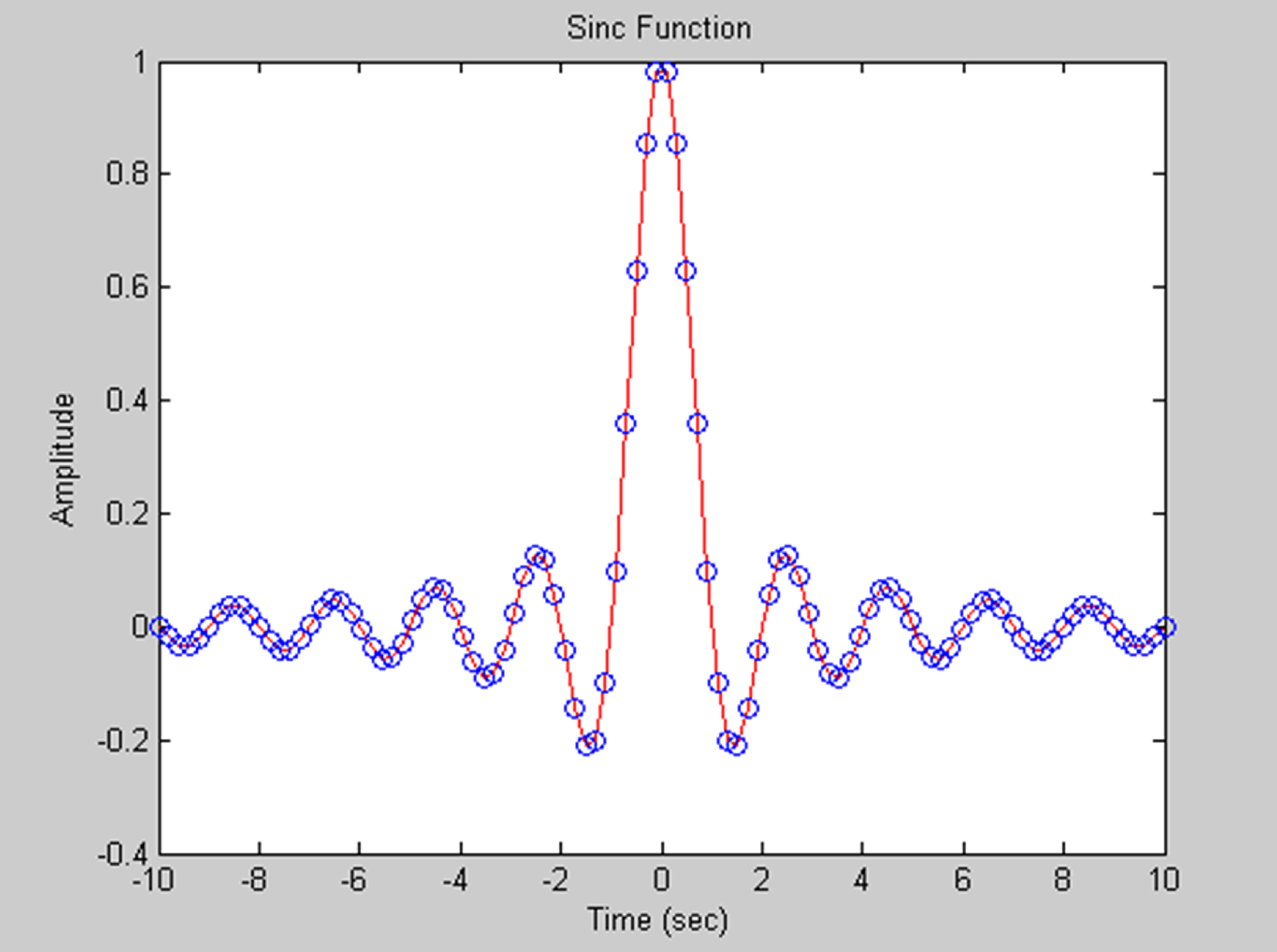
$C_{i} = (1 / 2 π) \cdot (1 / ji) \cdot 2 j sin (π i / 2) = (1 / 2 π i) \cdot sin (π i / 2)$ $C_{i} = (1 / 2 π) \cdot (1 / ji) \cdot 2 j sin (π i / 2) = (1 / 2 π i) \cdot sin (π i / 2)$

This expression gives the ideal response for a digital low-pass filter. The coefficients, which also represent the impulse response, decrease as 1/i as the coefficient index i gets larger. It is like a sine wave, with the amplitude gradually diminishing on each side. This function is called the sinc function, also known as sin(x)/x. It is a special function in DSP, because it gives an ideal low pass frequency response. The sinc function is plotted in Fig. 5.4, both as a sampled function and as a continuous function.

Our filter instantly transitions from passband to stopband. But before getting too excited about this filter, we should note that it requires infinite number of coefficients to realize this frequency response. As we truncate the number of coefficients (which is also the impulse response, which cannot be infinitely long in any real filter), we will get a progressively sloppier and sloppier transition from passband to stopband as well as less attenuation in the stopband. This can be seen in the figures below. What is important to realize is that to get a sharper filter response requires more coefficients or filter taps, which in turn requires more multiplier resources to compute. There will always be a trade-off between quality of filter response and number of filter taps, or coefficients.

5.4. Effect of Number of Taps on Filter Response

A picture is worth a thousand words or so it is said. Below are multiple plots of this filter with indicated number of coefficients. By inspection, you can see that as the number of coefficients grows, you will see actual |H(ω)| approaching desired |D(ω)| frequency response.

Filter plots are always given on a logarithmic amplitude scale. This allows us to see passband flatness, as well as see how much rejection, or attenuation, the filter provides to signals in its stopband.

All the following filter and coefficient plots are done using FIR Filter program. These filters can be easily implemented in FPGA or DSP processor.

Figure 5.5 7-tap ideal low-pass filter frequency response.

Above in Fig. 5.5 is a frequency plot of our ideal low pass filter. It does not look very ideal. The problem is that it is only 7 coefficients long. Ideally, it should be unlimited coefficients.

We can see some improvement in Fig. 5.6, with about twice the number of taps.

Now this is starting to look like a proper low-pass filter (Fig. 5.7).

You should notice how the transition from passband to stopband gets steeper as the number of taps increases. The stopband rejection also increases (Fig. 5.8).

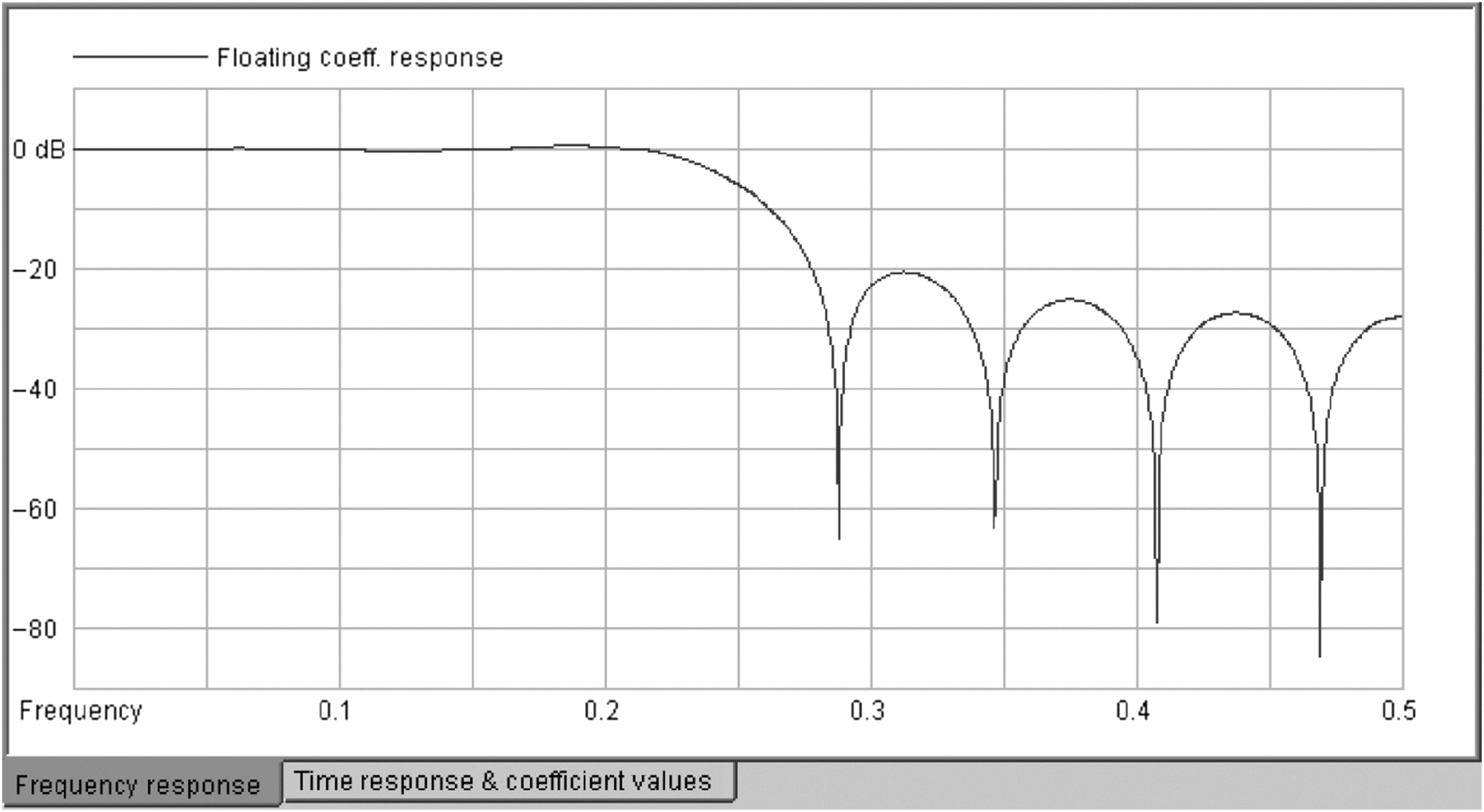
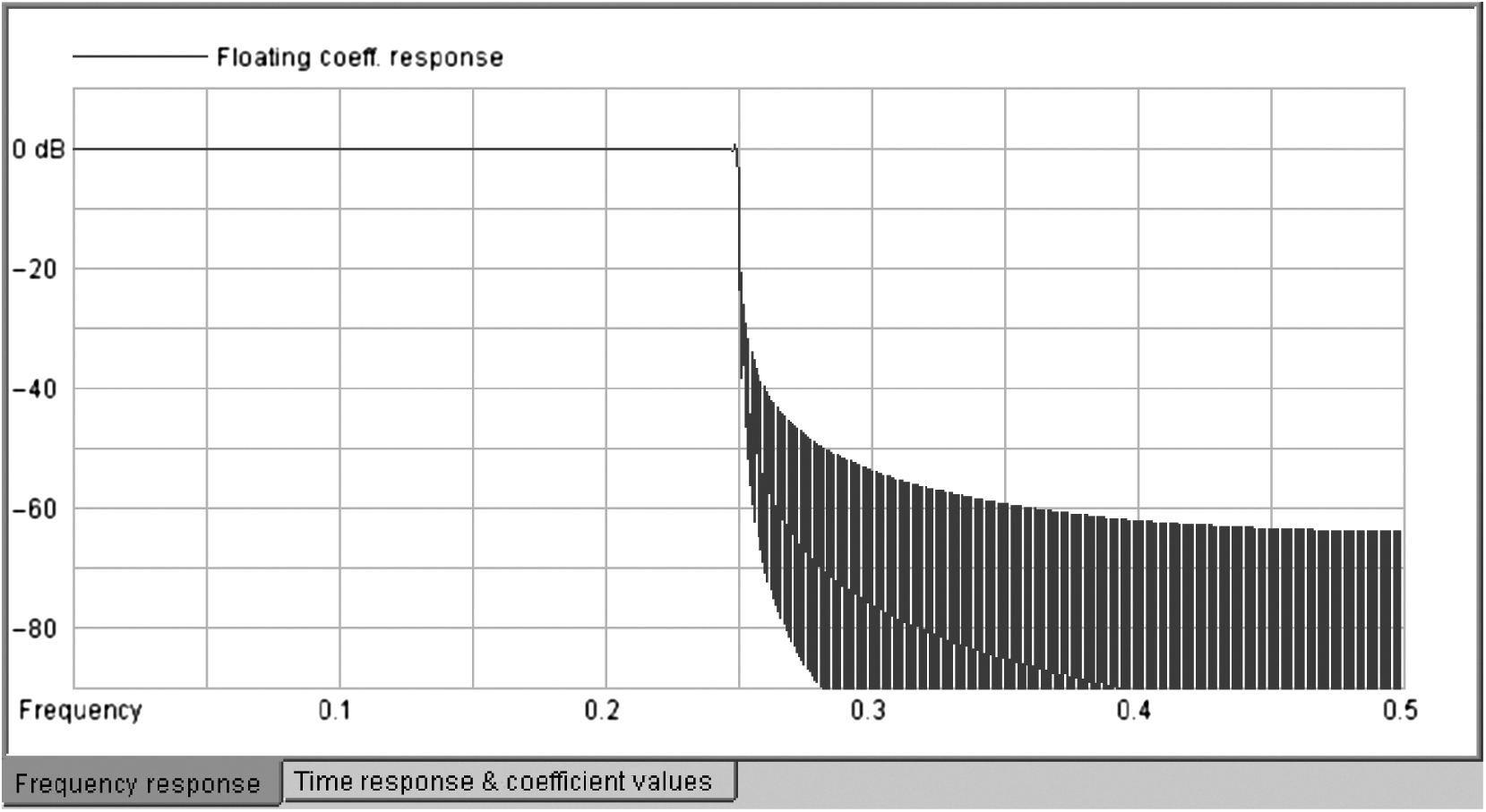
This is a very long filter, with closer to ideal response. Notice that how as the number of filter taps grow, the stopband rejection is increasing (it is doing a better job attenuating unwanted frequencies). For example, using 255 taps, by inspection |H(ω = 0.3)| ∼ −42 dB. With 1023 taps, |H(ω = 0.3)| ∼ −54 dB. Suppose a signal of frequency ω = 0.3 radians per second, with peak to peak amplitude equal to 1, is our input. The 255-tap filter would produce an output with peak to peak amplitude of ∼0.008. The 1023-tap filter would give 4x better rejection, producing an output with peak to peak amplitude of ∼0.002 (Fig. 5.9).

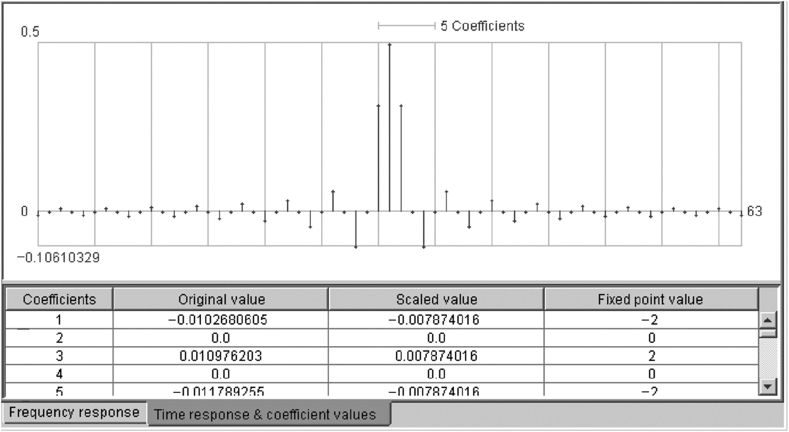
Above in Fig. 5.10 is the plot of the 63-tap sinc filter coefficients (this is not a frequency response plot). The sinc shape of the coefficient sequence can be easily seen. Notice that the coefficients fall on the zero crossing of the sinc function at every other coefficient.

Figure 5.6 15-tap ideal low-pass filter frequency response.

Figure 5.7 63-tap ideal low-pass filter frequency response.

Figure 5.8 255-tap ideal low-pass filter frequency response.

Figure 5.9 1023-tap ideal low-pass filter frequency response.

Figure 5.10 63-tap ideal low-pass filter coefficients.

There is one small point that might confuse an alert reader. Often a filter program will display the filter coefficients with indexes from −N/2 to N/2. In other cases, the same coefficients might be indexed from 0 to N, or from 1 to N+1. Our 5-tap example was {C₀, C₁, C₂, C₃, C₄}. What if we used {C₋₂, C₋₁, C₀, C₁, C₂}? These indexes are used in calculating the filter response, so does it matter how they are numbered or indexed?

The simple answer is no. The reason for this is that changing all the indexes by some constant offset has no effect on the magnitude of the frequency response.

Imagine if you put a shift register in front of your FIR filter. It would have the effect of delaying the input sequence by one sample. This is simply a one-sample delay. When a sampled signal is delayed, the result is simply a phase shift. Think for a moment about a cosine wave. If there is a delay of ¼ of the cosine period, this corresponds to 90°degrees. The result is a phase-shifted cosine, in this case a sine wave signal. This does not change the amplitude or the frequency, rather changes only the phase of the signal. Similarly, if the input signal or coefficients are delayed, this is simply a phase shift. As we saw previously, the filter frequency response is calculated as a magnitude function. There is no phase used in calculating the magnitude of the frequency response.

FIR filters will have a delay or latency associated with them. Usually, this delay is measured by comparing an impulse input to the filter output. We will see the output, starting one clock after the impulse input. This output or filter impulse response spans the length of the filter. So we measure the delay from the impulse input to the largest part of the filter output. In most cases, this will be the middle or center tap. For example, with our 5-tap example filter, the delay would be three samples. This is from the input impulse to the largest component of the output (impulse response), which is 5. In general, for an N-tap filter, where N is odd, the delay will be N/2 + 1. When N is even, it will be N/2 + ½. Since an FIR filter adds equal delay to all frequencies of the signal, it introduces no phase distortion, and it has a property called linear phase.

This is not as clear an explanation as you might like, but the essence is that since no phase distortion occurs when the signal passes through an FIR filter, we do not need to consider filter phase response in our design process. This is one reason why FIR filters are preferred over other types of digital filters.

The next chapter will cover with a topic called “windowing,” which is a method to optimize FIR filter frequency response without increasing the number of coefficients.

..................Content has been hidden....................

You can't read the all page of ebook, please click here login for view all page.

Table of Contents for Chapter 5. Finite Impulse Response (FIR) Filters

Create new playlist

Sign In