The main aim of this chapter is to reveal the function of the synthetic array radar (SAR). Normally, this radar is used to map ground features and terrain. It is also known in the literature as synthetic aperture radar. SAR can be an acronym for both. SAR systems can be designed with capabilities to differentiate using dimensions from few centimeters to hundreds of meters, depending on if the purpose is to map out a military installation—an urban area—or the contours of a mountain range. SAR radar is able to effectively create a very long antenna, hundreds of meters, using the motion of the aircraft. The radar is pulsed along this flight path, and the returns are digitally combined, to be able to view ground features with the resolution of a very long antenna. Hence the name “synthetic aperture” as the long antenna aperture is created through digital signal processing.
Synthetic array radar, or “SAR,” is normally used to map ground features and terrain. It is also known in literature as synthetic aperture radar. Both names make sense, though we use “Synthetic Array Radar” here. It is used for a wide variety of military and commercial applications. It can be made to map almost arbitrarily fine-resolution ground features or used to more coarsely map larger areas with comparative effort.
This process produces maps, which are often color coded. The color does not represent the actual color of the landscape but is used to indicate the strength of return signal for each resolvable location on the ground. Alternately, the images can be gray scale, with light regions indicating strong return and dark regions indicating little or no return. As different terrain features will reflect radar in differing amounts, features such as buildings, planes, rivers, roads, railroads, and so on can be seen in the SAR images. SAR radar is effective at night and in all weather, so if an effective complement to camera based imaging.
22.2. Synthetic Array Radar Resolution
The key parameter in ground mapping is the resolution. SAR systems can be designed with capabilities to differentiate using dimensions from few centimeters to a hundreds of meters, depending on if the purpose is to map out a military installation, an urban area, or the contours of a mountain range. The range is basically limited by the transmit power of the radar and can operate at resolutions much greater than visual, at long ranges and is unaffected by darkness, haze, or other factors impacting visual detection.
As with video, the quality of images depend on the pixel density (pixel stands for “picture element”). The equivalent of pixel density in radar is a voxel or “volume element.” The voxel is defined by the azimuth, elevation, and range. The minimum voxel size is dependent on the radar resolution capabilities. The voxel spacing is basically the distance that two points on the ground can be distinguished from each other. Radar resolution capabilities, in turn, are dependent on range resolution and main lobe beam width capabilities.
The voxel spacing or density should in general be at least 10 times the dimensions of the objects being mapped, to achieve useful images. A 1-m resolution is feasible for detecting buildings that are at least 10m long and wide.
As precision range detection is a fundamental requirement, high pulse repetition frequency (PRF) operation is unsuitable for SAR due to the range ambiguities. Low PRFs are used instead to eliminate range ambiguities over the distances from the aircraft to the ground being mapped. Maximum Doppler rates tend to be low, as the only motion is due to the radar-bearing aircraft motion. Owing to the nature of SAR, the relative motion is often substantially less than the aircraft flight speed. Use of a low PRF, while restricting the usable Doppler range, enhances the precision of Doppler frequency detection within that restricted range. This is an advantage in high-resolution SAR mapping.
22.3. Pulse Compression
Range resolution is dependent on the precision of the receive pulse detection arrival delay. This can be achieved by a very short transmit pulse width, which has the disadvantage of low transmit power level due to the short duration. Or very high levels of pulse compression can be used, which allow relatively long transmit pulses and therefore long integration times at the receiver, with the receiver operating on higher power returns. This raises the signal-to-noise power ratio (SNR) and allows for longer range mapping. A high level of pulse compression can be achieved by using long-matched filters (correlation to the complex conjugate of transmit sequence) and transmit sequences with strong autocorrelation properties. The only consequence is a higher level of computations associated with the long-matched filter. The speed of light, and therefore radar waves, is about 1m per 3ns (3×10⁻⁹). Since the path is round-trip, the range appears to become half of this. So for about 2m, or ∼6ft range resolution, requires a 12ns timing detection precision. To achieve this level of correlation would require a transmit sequence with phase changes of at least 80MHz rate, resulting at a minimum of the same amount transmit frequency bandwidth within the 10GHz radar band.
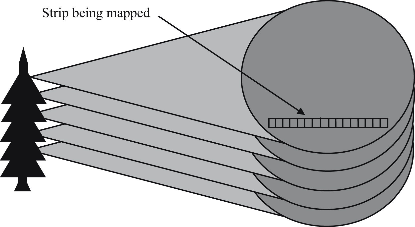
The elevation of the antenna main lobe does not need to be narrowly focused. In an SAR radar system, the antenna is directed to the ground at an angle off to the side, as shown in Fig. 22.1. As the elevation angle decreases, the radar beam will be directed at a steeper angle a ground location closer to the flight path of the aircraft, with a shorter range. The different portions of the beam elevation will therefore map to different ranges, and the return sequence can be directed into different range bins. The precision of the range detection capability translates into the degree of elevation resolution, often utilizing pulse compression.
22.4. Azimuth Resolution
The other requirement for precise ground mapping is a very narrow angular resolution of the main beam in the azimuth. As discussed in a previous chapter, the narrowness of the radar beam depends on the ratio of the antenna size to the wavelength. To achieve a “pencil”-like radar beam will require either a very large antenna or very high frequency (and short wavelength) radar. Both are impractical for airborne radar. The antenna size is necessarily limited by the aircraft size. Extremely high-frequency radars tend to be useful only at very short range, due to both atmospheric absorption and scattering. There is also the practicality of building high power and very high-frequency transmit circuits.
Figure 22.1 Synthetic array radar (SAR) range binning.
The solution to this is to create an artificially large antenna or synthetic array antenna. The forward motion of the aircraft is used to transmit and receive from many different points along the flight path of the aircraft. By focusing the radar main beam the same area of ground during the aircraft motion, the returns from different angles created by the aircraft motion can be synthesized into a very narrow equivalent azimuth main lobe using signal-processing techniques. The end result is as if an antenna of great length (up to a kilometer) was used. Because this is done using radar returns over several hundred milliseconds, this technique works for stationary targets, so is ideal for ground mapping.
SAR radar typically directs a radar beam at 90 degrees to the plane's flight path. The width of this radar beam does not have to be exceptionally narrow—in fact, the wider beam covers more ground and allows more processing gain in the SAR algorithm. When a large angle main lobe is used, the maximum length of the synthetic antenna is increased. Therefore, small antennas can work well with the SAR technique, as long as the antenna gain is sufficient to meet the SNR requirements for the range involved. The antenna will illuminate a large swath on the ground, typically an oval shape due to the aspect ratio of the beam being aimed outward from the aircraft flight path at downward angle.
To start with, let us assume that we can build an antenna as large as necessary to meet our azimuth resolution requirement. The rule of thumb governing antenna size is
dazimuth≈λR/L
where, dazimuth=resolvable distance in the azimuth direction, λ=wavelength of radar, R=range, L=length of the antenna.
(Note, for reasons not explained here, this expression is valid for conventional antennas. A SAR antenna actually has half the resolvable azimuth limit as a real antenna. In other words, a SAR antenna needs to be twice as large as a real antenna for the same resolvable distance).
If we need a 1-m aperture at a 10km range, with a 3cm (X band) radar, this requires an antenna length of 300m.
Imagine we had such an antenna, mounted along the fuselage of an impractically long 300m long plane. Each pulse could be focused with an azimuth width of 1m at the 10-km range, with a wide elevation, allowing the radar to scan narrow (1m) strip of land for each PRF, as the plane travels forward.
This 300-m long antenna could be composed of many radiating elements along this length (for example, 301 separate elements, spaced every meter). The antenna steering is accomplished by setting the phase of each element to ensure that the radar wave transmitted from each element is at a common phase when arriving at the 1-mstrip at 10-km distance. The phases will have to be adjusted, or focused, as the distance to the 1-mstrip of land will be slightly different for each element, due to the offset relative from the center element.
To aim the antenna beam at a very narrow region, the phase relationship of the different antenna elements must be carefully controlled. In our example, the wavelength is 3cm. If a radar round-trip path is 1.5cm longer or shorter than the middle element path, it will be 180 degrees out of phase and add destructively or cancel. Therefore the round-trip path length must be controlled within a few millimeters for each element. The phase error that occurs due to the plane's straight flight path as compared to an arc must be compensated for. This is shown below. The phase correction relative to the middle element of the antenna works is approximately as follows:
Θn=(2π⋅d2n)/(λ⋅R)
where, Θn=phase error of nth antenna element (in radians), dn=distance between middle element and nth antenna element. (In SAR literature, this term Θn is sometimes called the “point target phase history.”)
The return echo would be reflected from the ground at all locations and travel back to each element. Owing to the reciprocal path, it would arrive at the same phase offset that was transmitted, and if the same phase compensation is performed on the receive element signal prior to being summed together, the result will be that only the reflections from the 1-m width azimuth portion will arrive in phase, with all other ground returns being canceled out or at least severely attenuated.
Figure 22.2 Synthetic array radar pulse repition frequency effect.
Now suppose the same process is done in sequence, rather than all at once. We start with an element at the one end of the antenna and transmit a pulse and receive the return, using only this element. All the other elements are inactive. Both transmit and receive signals are modified by the phase compensation as before. The return sequence is stored in memory. Then we repeat this process with each separate antenna element in turn, until we have saved all the 301 return sequences. Remember, these return sequences are complex numbers, with a magnitude and phase. Now if we sum all the complex results at the end, we must have the same result as if we did everything in parallel at once. Nothing else has changed—the situation on the ground is assumed static. This is a simplified version of the process the SAR radar performs. Imagine as the plane flies forward, the PRF is such that 301 pulses are transmitted and received along 301m of flight path, as shown in Fig. 22.2.
The radar could then effectively map the 1-m wide strip at right angles to the flight path. However, while this solves the azimuth resolution problem, this is still not workable because only 1-m wide of strip ground is mapped perpendicular to the plane's flight path, every 301m.
22.5. Synthetic Array Radar Processing
To go further, we need some conventions. Let us assign an index to each 1-mstrip of land, oriented at right angles to the flight path, designated “n.” At the PRF when the aircraft is physically aligned with stripn, the real antenna will receive a complex range sequencen. This same index applies to the virtual or synthetic antenna element that is directly perpendicular to the 1-mstrip. The next synthetic antenna element forward would be index n+1, continuing on up to n+150. The synthetic antenna element behind would be n−1, extending to n−150. We will have complex weighting factors of proper phase and amplitude for each index, W−150 through W150. W0 is always equal to 1.
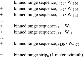
To calculate the image for stripn, we must start receiving range sequences at index n−150 and sort into range bins according to arrival time. This is using the single real antenna with wide beam angle (6–12degrees is typical). This will continue for 300 more PRF intervals, and result in 301 stored receive sequences in memory, indexed from −150 to +150. After PRF150, we can start processing. The 301 stored, binned range sequences will be multiplied or scaled by W−150 through W150, respectively. Note that both the values in the binned range sequences and the weighting factors are complex. Each range bin is multiplied separately by the weighting factor. Then the 301 complex range sequence results can then all be summed together across each range bin and will result in a range binned sequence which has an azimuth of 1m. The range bins correspond to the individual values across the elevation of the 1-m stripn.
For stripn+1, we wait until PRF151, and the plane has advanced 1m on its flight path. We can now start processing again. We have now just saved binned range sequence151 and can discard binned range sequence−150. This updated set of 301 binned range sequences is again multiplied by the weighting factors W−150 through W150. In this case, there is an offset as follows:
In this manner, we can compute each of the strips, one after the other, using a single broad beam antenna but using a long synthetic array to achieve a narrow azimuth. We can make the synthetic antenna arbitrarily long, by using more PRF cycles, more memory, and higher processing rates.
The signal processing achieves the same cancellation of signals coming from azimuths outside out desired 1-m ground strip as an actual 300-m antenna would do. This processing technique is known as line-by-line processing.
22.6. Synthetic Array Radar Doppler Processing
Another alternative method to perform SAR processing is to incorporate Doppler processing. Owing to the use of the efficient fast Fourier transforms (FFT) algorithm, this will lead to a much lower level of computations than line-by-line processing.
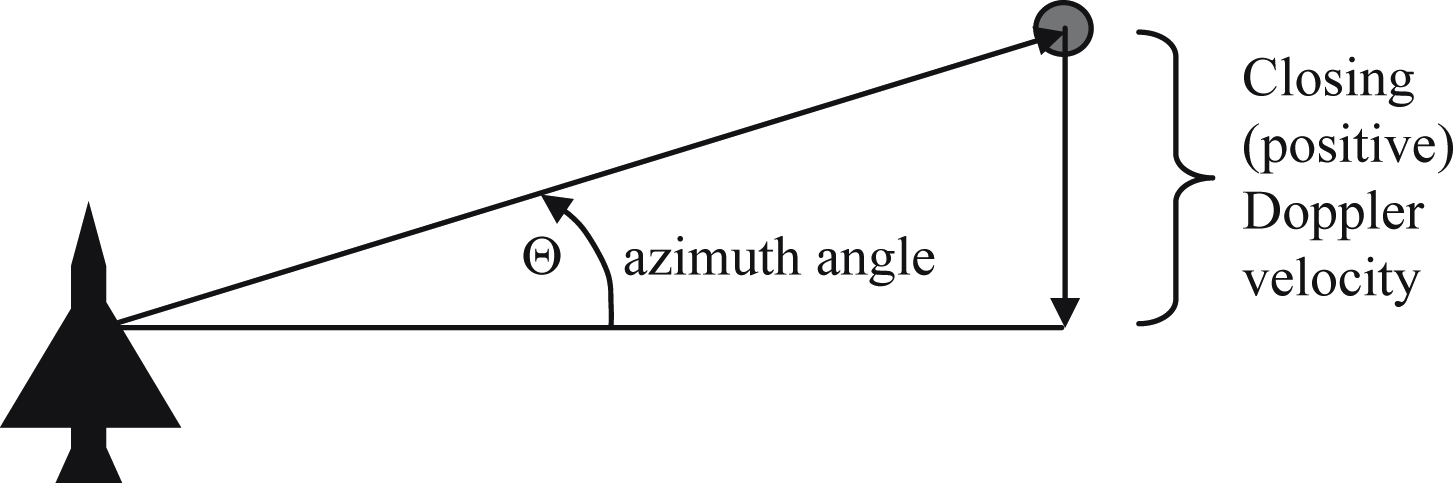
Consider the patch of ground being illuminated by the radar pulse directed at right angles to the aircraft flight path. This patch may be 2000m or more wide (azimuth direction), depending on the range and antenna beam width azimuth. At the midpoint, the Doppler frequency is exactly zero, as the radar is moving parallel to this point and has no relative motion. At the two azimuth end points of the scan area, we will have as follows:
As an example, with a range of 10km and a ground scan area of ±1000m, this equates to an angle of ±5.71 degree. If the aircraft is flying at 250m/s, this works out to ±829Hz in for the 10GHz radar band. This is shown in Fig. 22.3.
The Doppler frequency variation is not linear across the azimuth, due to the “sin (azimuth angle)” in the equation. At small angles, sin(θ)≈θ or approximately linear. As the angle increases, the effect becomes more nonlinear, until at 90degrees, the Doppler frequency asymptotically approaches the familiar (aircraft velocity/wavelength) or 8333Hz. However, we want the Doppler frequency response to be completely linear across the azimuth range. This can be compensated by using phase correction multiplier, known as “focusing.” The purpose is to make the Doppler frequency variation linear across the azimuth angle, rather than proportional to the sine of the angle. Once the frequency spacing per unit length on the ground is made linear, it allows us to use Doppler filters with equally spaced main lobes along the frequency axis. This filtering is the familiar discrete fourier transform, which can be implemented using the FFT algorithm. This is known as SAR Doppler processing. The advantage of this is that the computational load is made much more manageable than the line-by-line processing technique, by virtue of the FFT algorithm efficiency.
Figure 22.3 Synthetic array radar Doppler effect.
As a side note, this Doppler linearity is an issue only for SAR radar. For conventional radar, the radar is aimed toward the horizon, and there is less variation due to the aspect angles (in this case, θelavation is close to 0°, although θazimuth can have significant variation), and the sensitivity requirements are much less for SAR.
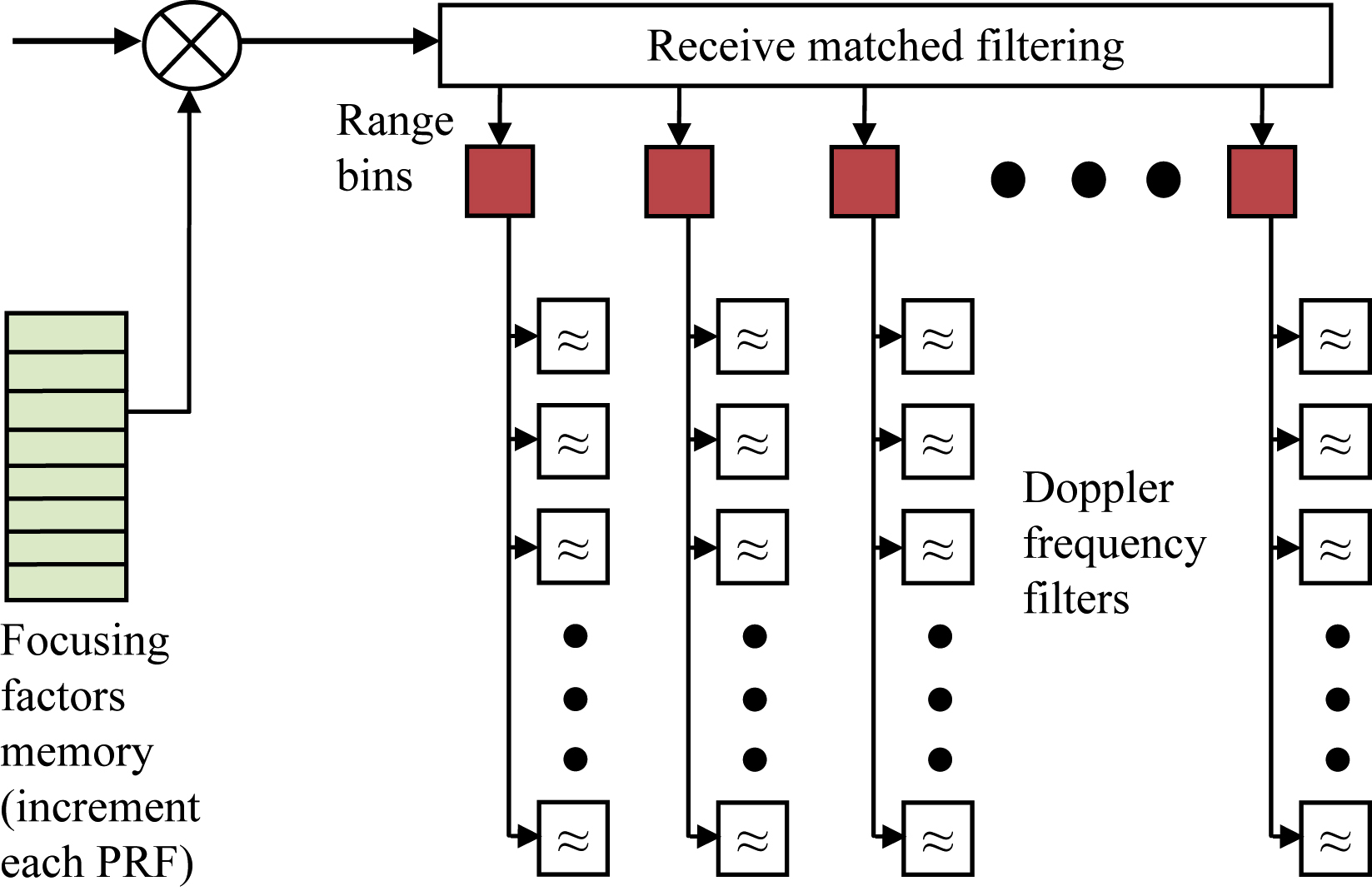
At each PRF, the return sequence is multiplied by a phase correction (focusing). Each range bin stores a complex value, representing the phase and magnitude of the return at that range. For each range, the values are loaded into all the Doppler frequency filters matching the azimuth angles for each ground element, as shown in Fig. 22.4.
Each pulse has its return processed by azimuth and range, which allows separation over all locations in the radar beam, with resolution determined by the number of range bin and Doppler filter frequency banks. This is repeated at each PRF with the next phase correction value, and the results are accumulated or integrated. Over the set of N PRFs equal to the number of N elements in the synthetic antenna, this is repeated.
After each set of N PRFs, the process repeats. The same point is measured N times, and complex values representing both magnitude and phase are integrated over the measurements for each point. In this architecture, the number of virtual elements in the synthetic array is equal to the number of Doppler filters, which can also be set equal to the number of range bins. This is also the number of times each point is measured, and the results integrated. However, each of the different measurements for a given point is done at a different azimuth angle.
In reality, these two methods provide equivalent results, although the processing steps are different. The first method is conceptually easier for most people to understand. The second method has the advantage of lower computational rate. An intuitive Fig. 22.5 that depicts the two different approaches is shown.
An alternative way to understand this is that line by line, a new narrow beam at right angles to the flight line is synthetically created for each PRF. With Doppler processing, many different azimuth beams are generated by each Doppler frequency bank during each PRF, and the returns from each beam are summed over multiple PRFs. Mathematically, a process called “back-projection” is used to create the SAR image, but this is not covered in this introductory treatment.
22.7. Synthetic Array Radar Impairments
Several factors can degrade SAR performance. One of the most significant is nonlinear flight path of an aircraft. We have seen how sensitive the phase alignments are to proper focusing, in fractions of the radar wavelength. Therefore, deviations in flight path away from the parallel line of the radar scan path must be determined and accounted for. This motion compensation can be done using inertial navigation equipment and by using GPS location and elevation measurements. Another consideration is side lobe return. When the side lobe return from the ground beneath the plane is integrated over a wide azimuth and elevation angles, this can become significant despite the low antenna gain at the side lobes. The design of the synthetic antenna, just like a real antenna, must take this factor into account. There are methods, similar to windowing in finite impulse response filters, which can reduce side lobes, but at the expense of widening the main lobe and degrading resolution. Another issue is that the central assumption in SAR is that the scanned area is not in motion. If vehicles or other targets on the ground are in motion, they will not be resolved correctly and be distorted in the images. Shadowing is another impairment. This occurs when a tall object shields other object from the radar's illumination, causing a block or blank spot in the range return. This becomes more prevalent when very shallow angles are used—which occurs when the aircraft is at low altitude and scanning at long ranges. At high altitudes, such as satellite-mounted SAR, this is much less of an issue.
Figure 22.5 Synthetic array radar (SAR) integration over pulses.