
Chapter 7
Decimation and Interpolation
Abstract
The chapter discusses the process of decimation and interpolation in a signal processing system. Implementation is done using a finite impulse response (FIR) filter, which allows reducing and increasing the sample rate. The frequency domain view of decimation and interpolation is explained. It also discusses situations of high oversampling of a signal, resampling of noninteger value, and the interpolation effects. It concludes with explanation of resampling by a noninteger rate.
Keywords
Analog to digital converter; Decimation; DSP processors; Finite impulse response; Low-pass filter
In this chapter, we are going to discuss decimation and interpolation. Decimation is the process of reducing the sample rate Fs in a signal processing system, and interpolation is the opposite, increasing the sample rate Fs in a signal processing system. This process is very common in signal processing systems and is nearly always performed using a finite impulse response (FIR) filter.
First of all, why are sampling rates changed? The most common reason is that higher sample rates make it easier in the analog domain, whereas lower rates reduce the digital computational requirements. The ADCs and DACs often operate a higher frequency, while most filtering and other functions can be operated at a lower frequency. As we have seen in previous chapters, signals have a frequency representation, and this frequency representation must be less than the Nyquist frequency, which is defined as Fs/2. This sets a lower bound on Fs. The amount of hardware or software processing resources is normally proportional to Fs, so we usually want to keep Fs as small as practical. So while there is no upper bound on Fs, it is usually less than 10× the frequency representation of the signal. A minimum Fs is needed to ensure the highest frequency portion of the signal does not approach the FNyquist frequency.
In some cases, there are advantages to highly oversampling a signal, where Fs >> Fsignal. One such example might be when sampling a signal using an analog to digital converter (ADC). If Fs is high, then so is FNyquist. Recall that we can accurately represent all signals below FNyquist in the sampled domain without aliasing occurring. By making FNyquist large, any unwanted signals in that frequency space can be eliminated, or at least highly attenuated, by using a digital filter with its passband matching our desired frequency and with its stopband for the rest of frequency spectrum up to FNyquist. The analog filter needs to filter out frequencies above FNyquist. In this manner, by increasing Fs and therefore FNyquist, we can simplify the requirements for analog filtering prior to the ADC. Now once we have successfully filtered out these unwanted signals through both the analog and digital filters, we have no further need of keeping the Fs >> Fsignal and should consider lowering Fs to reduce resources required for subsequent processing.
7.1. Decimation
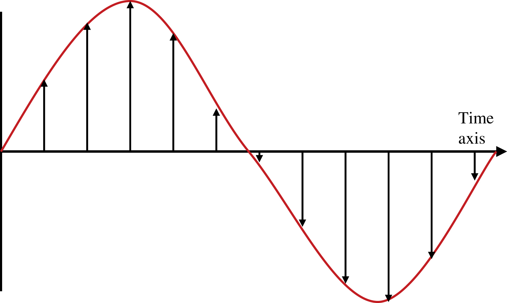
To discuss decimation, or down sampling as it is also called, we need to consider the frequency representation of the signal as well as the time domain. First we will look at the sampled signal sampled at Fs (Fig. 7.1) and at  , where
  (Fig. 7.2). The new sampling rate is the sampling rate after decimating by 2.

Below in Fig. 7.3, is the frequency domain perspective of decimation.
By examining the frequency plots, it is evident the signal itself has not changed, only the sampling rate frequency and corresponding Nyquist rate frequency. As long as the new Nyquist frequency is larger than the signal frequency, no aliasing will occur.
The signal images, which are periodic in Fs, and a natural consequence of sampling, are also shown. When decimating, the images become periodic in the new sample rate .
One could decimate by simply throwing away samples. In our example, by throwing away every other sample, the sample rate will be reduced by a factor of ½, and result will be as shown above.


In practice, however, the decimation process usually has a low-pass filter (LPF) incorporated. Let us go back to our ADC example. This could be implemented using the block diagram in Fig. 7.4. In this example, the analog LPF is responsible for removing all unwanted signals above FNyquist, which would otherwise alias into the frequency region where our signal is. With this analog LPF prior to the ADC, we can then be confident that any signals we see below FNyquist are legitimate signals, and not aliased versions of some higher frequency unwanted signal or noise. We must similarly provide an LPF prior to the decimator, to remove any frequency components between  and , else any frequency components in this frequency band will alias, or fold back, into the frequency band below our new Nyquist frequency . The approximate frequency response of the analog and digital LPF is depicted in the previous frequency domain (Fig. 7.3).
Now we can ask an interesting question. Why bother to compute samples at rate Fs in the digital LPF if we are going to discard ½ of them in the decimator? This is a waste of processing resources. Instead, we can build a digital filter which only computes every other sample, and therefore accomplishes the function of the decimator (shown separately in our block diagram). And in the process, we find that we only need one half the multiplier rate to implement the digital LPF.

To see how we might do this, we will reconsider the FIR block diagram Fig. 7.5.
In the normal case, at each clock cycle, the xk data advance into the shift register of the filter structure, and an output yk is produced. As we did earlier, one can build a sequence of inputs and compute the sequence of outputs. The filter equation is repeated below:
Now suppose that on every even clock cycle (k is even), we operate the filter normally, but on the odd clock cycles (k is odd), we merely shift the input data, but disable the operation of multipliers, summation, and update of output register (this register not explicitly shown). The output register will just hold the previous value, since there has been no update.
We will show how to compute a few outputs,
(y1 output not computed, only xk input data shifted through)
(y3 output not computed, only xk input data shifted through)
And so forth.
The output sequence is the decimated, filtered sequence {… y0, y2, y4,…}. Only the shift registers operate at the input rate. The rest of the circuitry can be clocked at the output clock rate. If implemented using DSP processors, or if you are clever in your hardware filter design, you can utilize less multipliers by operating them at the faster input speed. This is beyond our scope here, but in general, whether implementing DSP algorithms in hardware (FPGA or ASIC) or in software (DSP processor), the multipliers can be multiplexed such that it does not matter whether you have a few very fast multipliers, or a large number of slow multipliers or anything in between, so long as the cumulative multiply-accumulate capacity is sufficient for the DSP algorithm requirement.
Decimation is limited to integer values. So this concept can be extended to decimate by 3, 4, 10, and so forth. In each case, the decimation filter only computes the required samples. The input data is shifted right by the decimation rate between each computation. In our decimate-by-2 example above, the input data is shifted right by two places between each output computation (check the x indexes in the example computations above).
7.2. Interpolation
As we just saw, decreasing the sample rate Fs by an integer value can be accomplished by a decimation FIR filter. Similarly, the sample rate Fs can be increased by an integer value using a type of FIR filter called an interpolation filter. This is called upsampling and is the opposite of decimation. As long as the signal frequency content is below the Nyquist frequency at the lowest sampling frequency, one can decimate a signal and then turn around and interpolate it and recover the same signal.
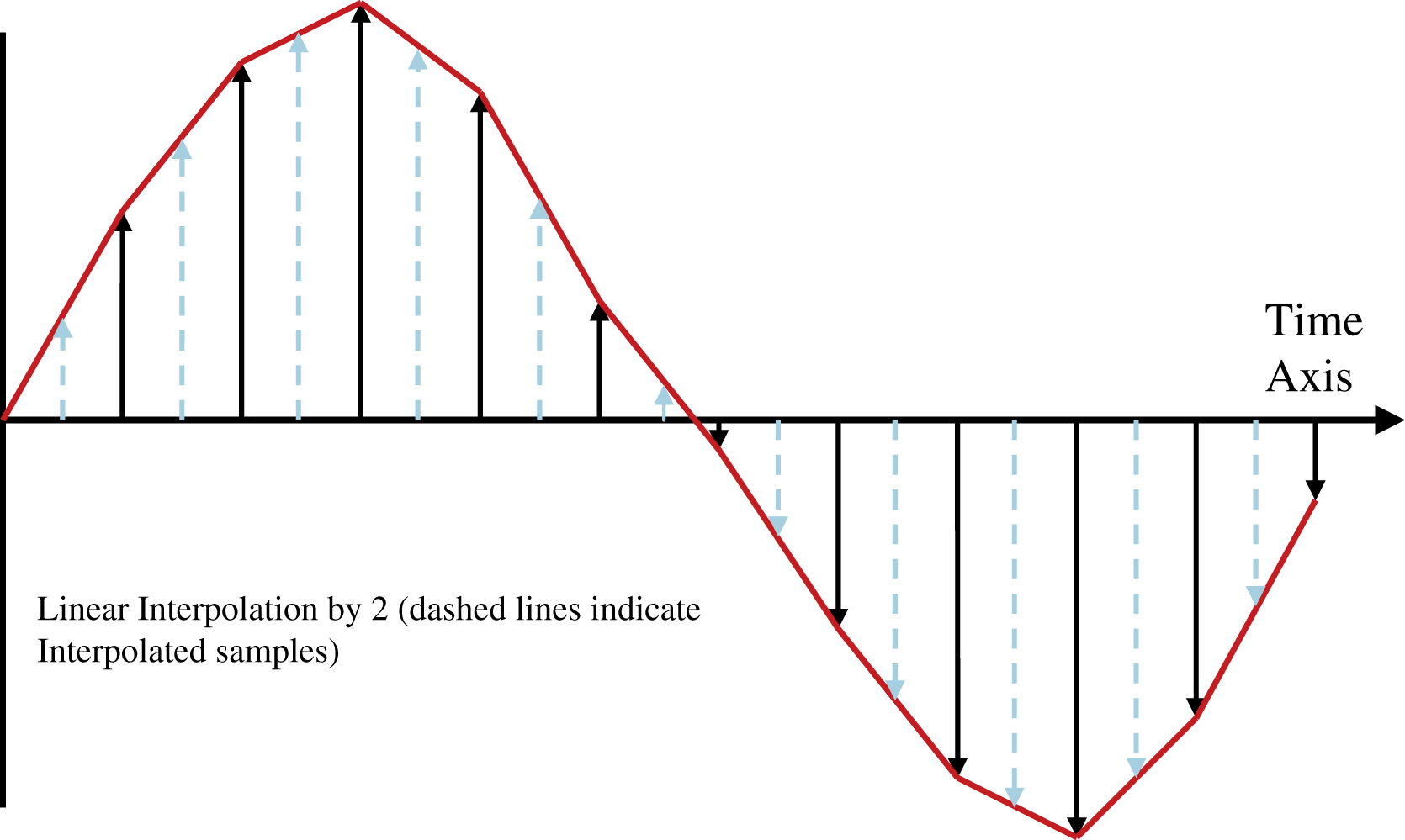
Interpolation requires that the sample rate be increased by some integer factor. New samples need to be created and inserted between the existing samples. Let us look at the simplest example of interpolation. Let us go back to our sine wave example and interpolate it by a factor of two in Fig. 7.6.

Shown is the original signal at sample rate Fs where the “triangles” indicate approximately where new samples must be created to interpolate up to sample rate  . This seems straight forward enough. We do not have to worry about aliasing issues, because we are doubling both the sample frequency and Nyquist frequency.
The simplest and most intuitive way to interpolate is called linear interpolation. In linear interpolation, one simply draws a straight line between the original samples, and calculates the new samples along this line. In our case, if we interpolate by 2, then we need the point located mid-way along the line between the original points. Linear interpolation, whether by factor of 2, 3, 4, … is equivalent to drawing a line between all the original points, and will look something like the following figure.
Signal at shown in Fig. 7.7 with linear interpolation. Obviously, this does not look quite right. But let us consider how we would build an interpolation filter.
An interpolation filter is actually several filters running in parallel, each with the same data input xk. Each filter computes a different intermediate sample. One filter has a single tap = 1, which provides the original signal at the output (this could just be a shift register to provide correct delay). Each of the other filters calculates one of the new samples between the original samples. When interpolating by N, there will be N of these filters, including the trivial filter that generates the original samples. For example, when interpolating by four, N = 4, and there will be four of these filters. Every input sample will produce four output samples, one from each filter, which will be interleaved at the output at a combined rate four times larger than the input rate. This concept, of multiple filters creating a single output with higher rate sequence, is called polyphase filtering.
The length or number of taps in each of the N interpolation filters will largely determine the quality of the interpolation. With linear interpolation, the number of filter taps is only 2, so the quality of the interpolated signal is rather poor, as can be seen above. The ideal filter is an LPF with cutoff frequency at FNyquist of the original signal sampling rate. As we learned previously, an ideal filter has infinite number of coefficients. We will have to compromise at less than infinity, and so each individual filter will have M taps.
Shown in Fig. 7.8 is an interpolate-by-4 (N = 4) polyphase filter, with 5 taps (M = 5) used for each phase. The input data stream xk is sampled at Fs, and the serialized output data stream ym is sampled  . Coefficient representations An, Bn, and Cn are used to indicate that each phase of the interpolation filter may have a different set of coefficients.
You should note how the first filter could be eliminated and replaced by a shift register. All of the taps except the center one are multiplying by zero, so the multiplier and adder logic is not required. The original input sample simply passes through with some delay.
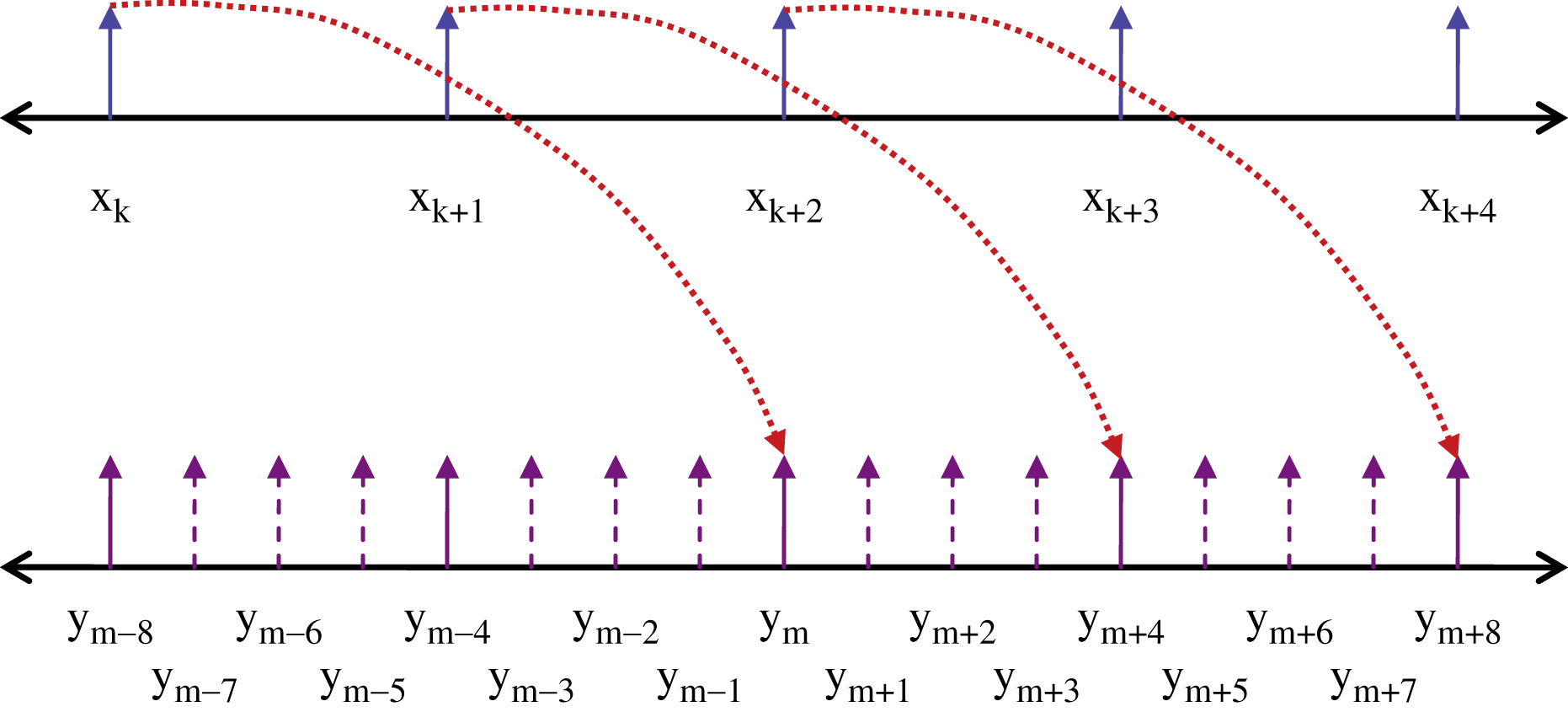
Interpolating polyphase filters are a little tricky, so we will also show what is happening in the time or sample domain. Shown below in Fig. 7.9 is the input and output sequences, which are time aligned for clarity. The output data rate is four times the input, and like all FIR filters, there is some processing delay through the filter. The function of the serializer is to input N samples in parallel at rate Fs, and output a serial sample stream at , which is the new interpolated sample rate.
The dashed lines indicate the interpolated samples. The dotted lines show the delay of the original samples through the interpolation filter. This delay is dependent on filter design, but is generally equal to (M − 1)/2 input samples, plus any additional register pipeline delays. In our example above, M = 5, so the delay is (5 − 1)/2 = 2 input sample intervals.
Note that the “m” output index is increasing faster than the “k” input index. The interpolation filter must produce N output samples for every input sample, so the output index “m” needs to run N times faster than “k”.
7.3. Resampling by Noninteger Value
Suppose that you need to align the sample rates between sets of digital circuitry running at different sampling rates. For example, the sampling rate of the first circuit is 3 MSPS, and the second circuit has a sampling rate of 2 MSPS. You will need to decimate, or downsample, by 2/3.
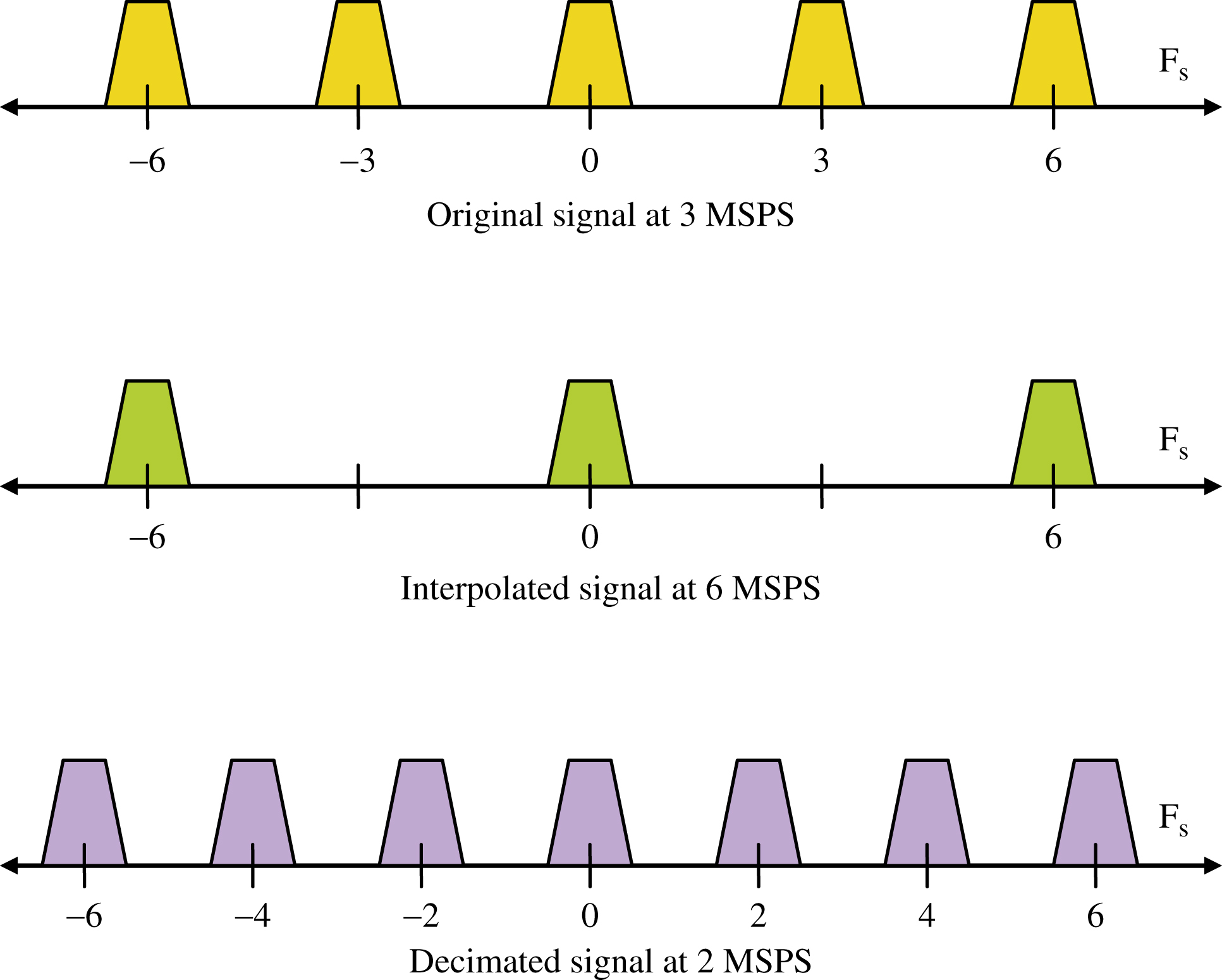
This can be done by a combination of interpolating and decimating. In this case, you would interpolate by 2 and then decimate by 3, as shown in Fig. 7.10.
Next, a frequency domain representation of both interpolation and decimation steps is shown in Fig. 7.11.

Both the interpolation and decimation filters incorporate a low-pass filtering function. The reason for this LPF, however, is quite different for each case. For decimation, the LPF serves to eliminate high frequency components in the spectrum. If these components were not filtered out, they would alias when the reduction in sample rate is performed.

For interpolation, the LPF serves to provide a “smoothing” function when calculating the new samples, so that a smooth curve results when the new samples are inserted between the original samples. A longer interpolating filter (more taps = larger M) will use a weighted calculation of larger number of the adjacent samples to determine the new samples. An analogy might be when a person is driving a car on a winding road. If you look only a few feet in front of the car, you cannot take the curves smoothly. The reason is that since you are not looking ahead, you cannot anticipate the direction and rate of curves and smoothly adjust to it. The interpolating filter works best when it can look at samples on both sides (or in front and behind) when computing the new samples, which should smoothly fit in between the existing samples.
When M = 2, which is linear interpolation, only the two adjacent samples are used, and the filter computes the sample which lies on a straight line between the two points. As we saw in the example, this does not give a very smooth response. This lack of smooth response can also create some higher frequency components in the signal spectrum. If M = 4, then the filter uses four samples, two on either side, to compute the new samples. As M becomes larger, the interpolated response improves, both in time domain and frequency domain. To achieve perfect interpolation, you would need to use an infinite number of samples, and build a perfect LPF. This perfect interpolation filter would be in the form of the sinc function, also known as  , introduced in the FIR Filter chapter, and be of infinite length. In practice, using between 8 and 16 samples, or filter coefficients, is usually enough to a reasonable job of interpolating a signal for most applications.
..................Content has been hidden....................
You can't read the all page of ebook, please click here login for view all page.